Learnable Manifold Alignment (LeMA) : A
1
Semi-supervised Cross-modality Learning Framework for
2
Land Cover and Land Use Classification
3
Danfeng Honga,b, Naoto Yokoyac, Nan Gea, Jocelyn Chanussotd, Xiao Xiang Zhua,b,∗
4
aRemote Sensing Technology Institute (IMF), German Aerospace Center (DLR), Wessling, Germany
5
bSignal Processing in Earth Observation (SiPEO), Technical University of Munich (TUM), Munich,
6
Germany 7
cGeoinformatics Unit, RIKEN Center for Advanced Intelligence Project (AIP), RIKEN, Tokyo, Japan
8
dUniv. Grenoble Alpes, CNRS, Grenoble INP, GIPSA-lab, Grenoble, France
9
Abstract
10
In this paper, we aim at tackling a general but interesting cross-modality feature learn-ing question in remote senslearn-ing community —can a limited amount of highly-discrimin-ative (e.g., hyperspectral) training data improve the performance of a classification task using a large amount of poorly-discriminative (e.g., multispectral) data? Tradi-tional semi-supervised manifold alignment methods do not perform sufficiently well for such problems, since the hyperspectral data is very expensive to be largely col-lected in a trade-off between time and efficiency, compared to the multispectral data. To this end, we propose a novel semi-supervised cross-modality learning framework, called learnable manifold alignment (LeMA). LeMA learns a joint graph structure di-rectly from the data instead of using a given fixed graph defined by a Gaussian ker-nel function. With the learned graph, we can further capture the data distribution by graph-based label propagation, which enables finding a more accurate decision bound-ary. Additionally, an optimization strategy based on the alternating direction method of multipliers (ADMM) is designed to solve the proposed model. Extensive experiments on two hyperspectral-multispectral datasets demonstrate the superiority and effective-ness of the proposed method in comparison with several state-of-the-art methods. Keywords:
11
Cross-modality, graph learning, hyperspectral, manifold alignment, multispectral,
12
remote sensing, semi-supervised learning.
1. Introduction
14
Multispectral (MS) imagery has been receiving an increasing interest in the urban
15
area (e.g. a large-scale land-cover mapping [1] [2], building localization [3]),
agri-16
culture [4], and mineral products [5], as operational optical broadband (multispectral)
17
satellites (e.g. Sentinel-2 and Landsat-8 [6]) enable the multispectral imagery openly
18
available on a global scale. In general, a reliable classifier needs to be trained on a
19
large amount of labeled, discriminative, and high-quality samples. Unfortunately,
la-20
beling data, in particular large-scale data, is very gruelling and time-consuming. A
21
natural alternative way to this issue is to consider tons of unlabeled data, yielding a
22
semi-supervised learning. On the other hand, MS data fails to spectrally discriminate
23
similar classes due to its broad spectral bandwidth. A simple way is to improve the data
24
quality by fusing high-discriminative hyperspectral (HS) data [6]. Although such data
25
is expensive to collect, we may be able to expect a small amount of such data available.
26
The aforementioned two points motivate us to raise a question related to transfer
learn-27
ing and cross-modality learning: Can a limited amount of HS training data partially
28
overlapping MS data improve the performance of a classification task using a large
29
coverage of MS testing data?
30
Over the past decades, land-cover and land-use classification tasks of optical
re-31
mote sensing imagery has received increasing attention in the unsupervised [7] [8] [9],
32
supervised [10] [11], and semi-supervised ways [12] [13]. To our best knowledge,
33
the classifying ability in unsupervised learning (or dimensionality reduction) still
re-34
mains limited, due to missing label information. By fully considering the variability of
35
intra-class and inter-class from labels, supervised learning is able to perform the
clas-36
sification task better. In reality, a limited number of labeled samples usually hinders
37
the trained classier towards a high classification performance, further leading to a
pos-38
sible failure in some challenging classification or transferring tasks owing to the lack
39
of generalization and representability. Alternatively, semi-supervised learning draws
40
into plenty of unlabeled data in learning process. This is capable of better capturing
41
the distribution of different categories in order to find an accurate decision boundary.
On the other hand, considerable work related to transfer learning (TL) or domain
43
adaptation (DA) has been successfully developed and applied in the remote sensing
44
community [14, 15, 16, 17, 18, 19]. According to the different transferred objects, the
45
TL or DA approaches can be roughly categorized into three groups, including
parame-46
ter adaptation, instance-based transfer, and feature-based alignment or representation.
47
The seminal work dealing with parameter adaptation was presented in [20] and
48
[21], aiming at transferring an existing classifier (or parameters) trained or learned
49
from the source domain to the target domain. Differently, the instance-based
trans-50
ferring technique transfers the knowledge by reweighting [22] or resampling [23] the
51
samples of the source domain to those of the target domain. A similar idea based on
52
active learning [24] has also been proposed to address this issue, by selecting the most
53
informative samples in the target domain to replace with those samples of the source
54
domain that do not match the data distribution of the target domain [25].
55
For the final group of feature-based alignment or representation, manifold
align-56
ment (MA) is one of the most popular semi-supervised learning framework [26] that
57
facilitates transfer learning. MA has been successfully applied to various tasks in
58
remote sensing community, e.g. classification [27], data visualization [28],
multi-59
modality data analysis [13], etc. The key idea of MA can be generalized as learning a
60
common (or shared) subspace where different data can be aligned to learn a joint
fea-61
ture representation. Generally, existing MA methods can be approximately categorized
62
into unsupervised, supervised, and semi-supervised approaches. The unsupervised
ap-63
proach usually fails to align multimodal data sufficiently well, as their corresponding
64
low-dimensional embeddings may be quite diverse [29]. In the supervised case, only
65
aligning the limited number of training samples to learn a common subspace leads to
66
weak transferability. While preserving a joint manifold structure created by both
la-67
beled and unlabeled data, semi-supervised alignment allows different data sources to
68
be better transformed into the common subspace [30].
69
Although the joint manifold structure used in conventional semi-supervised MA
70
approaches can relate features or instances, poor connections between the common
71
subspace and label information still hinder the low-dimensional feature
representa-72
tion from being more discriminative. More importantly, in most graph-based
supervised learning algorithms (e.g. graph-based label propagation (GLP) [31],
semi-74
supervised manifold alignment (S-SMA [13]) [30]), the topology of unlabeled samples
75
is merely given by a fixed Gaussian kernel function, which is computed in the original
76
space rather than in the common space. This makes it difficult to adaptively transfer
77
unlabeled samples into the learned common subspace, particularly when applied to
78
multimodal data due to different numbers of dimensions. To address these issues, we
79
propose a learnable manifold alignment (LeMA) by a data-driven graph learning
di-80
rectly from a common subspace so as to make the multimodal data comparable as well
81
as improve the explainability of the learned common subspace, which further results
82
in a better transferability. More specifically, our contributions can be summarized as
83
follows:
84
• We propose a novel semi-supervised cross-modality learning framework called
85
learnable manifold alignment (LeMA) for a large-scale land-cover classification
86
task. One spectrally-poor MS and one spectrally rich HS data are considered as
87
two different modalities and applied for this task, where the spatial extent of the
88
former is a true superset of that of the latter.
89
• Unlike jointly feature learning in which the model is both trained and tested from
90
completed HS-MS correspondences, LeMA learns an aligned feature subspace
91
from the labeled HS-MS correspondences and partially unlabeled MS data, and
92
allows to identify out-of-samples using either MS data or HS data; Such the
93
learnt subspace is a good fit for our case of cross-modality learning1. 94
• Instead of directly computing graph structure with a Gaussian kernel function, a
95
data-driven graph learning method is exploited behind LeMA in order to strengthen
96
the abilities of transferring and generalization;
97
• An optimization framework based on the alternating direction method of
multi-98
pliers (ADMM) is designed to fast and effectively solve the proposed model.
99
1In contrast to multi-modal learning (bi-modality for example), cross-modal learning trains on single
Multispectral Data
Unlabeled Multispectral Data
Labels Computed by LabelsJoint Graph
Learnable Manifold Alignment
Labeled Samples
Joint Feature Learning
Joint Graph Learned from
Labeled and Unlabled Data Common Subspace
Unlabled Features Labled Features Labeled Data etc.
Classification
Multispectral Hyperspectral Same Area
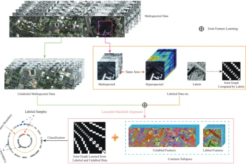
Figure 1: An illustration of the proposed LeMA method.
The remainder of this paper is organized as follows. Section II elaborates on our
100
motivation and proposes the methodology for the LeMA and the corresponding
opti-101
mization algorithm. In Section III, we present the experimental results on two HS-MS
102
datasets over the areas of the University of Houston and Chikusei, respectively, and
103
meanwhile discuss the qualitative and quantitative analysis. Section IV concludes with
104
a summary.
105
2. Learnable Manifold Alignment (LeMA)
106
In this section, a cross-modality learning problem is firstly casted and the
moti-107
vation is stated in the following. Accordingly, we formulate the methodology of our
108
proposed and then elucidate an ADMM-based optimization algorithm to solve it.
109
2.1. Problem Statement and Motivation
110
For many high-level data analysis tasks in remote sensing community, such as
111
land-cover classification, data collection plays an important role, since
information-112
rich training samples enable us to easily find an optimal decision boundary.
WMM WHH XH XM XM XH XU XU WMH WHM WUH WUM WHU WMU WUU
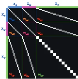
Figure 2: An example for the joint adjacency matrixWf.
There is, however, a typical bottleneck in collecting a large amount of labeled and
114
discriminative data. Despite the MS data available at a global scale from the
satel-115
lites of Sentinel-2 and Landsat-8, the identification and discrimination of materials are
116
unattainable at an accuracy level by MS data, resulting from its poorly spectral
infor-117
mation. On the contrary, HS data is characterized by rich spectral information, but only
118
can be acquired in very small areas, due to the limitations of imaging sensors. This
is-119
sue naturally guides us to jointly utilize the HS and MS bi-modal data, specifically
120
leading to the following interesting and challenging questioncan a limited number of
121
HS training data contribute to the classification task of a large-scale MS data?
122
A feasible solution to the issue can be unfolded to two parts: 1)cross-modality
123
learning: learning a common subspace where the features are expected to absorb the
124
different properties from the HS-MS modalities and meanwhile the HS and MS data
125
can be transferred each other; 2)semi-supervised learning: Embedding massive
unla-126
beled MS samples which are relatively in large quantities and easy to be collected, so
127
as to learn a more discriminative feature representation. Fig. 1 illustrates the workflow
128
of LeMA.
2.2. Problem Formulation
130
To effectively model the aforementioned issue, we intend to develop a joint learning
131
framework which better learns a discriminative common subspace from high-quality
132
HS data and low-quality MS data. Intuitively, such a common subspace can be shaped
133
by selectively absorbing the benefits of both high-quality data with more details and
134
low-quality data with more structural information. Therefore, following a popular joint
135
learning framework [32], we formulate the common subspace learning problem as
136 min P,Θ 1 2kYe −PΘXke 2 F+ α 2kPk 2 F+ β 2 tr(ELE T) s.t.E=Θ e X, ΘΘT=I, (1)
whereYe = [Y,Y] ∈ Rd×2N andY ∈ Rd×N is the label matrix represented by
137 one-hot encoding,Xe = XH 0 0 XM
∈R(dH+dM)×2N andXH andXM stand re-138
spectively for the data from hyperspectral and multispectral domains,Θ= [ΘH,ΘM] 139
andPare respectively the common subspace projection and the linear projection to
140
bridge the common subspace and label information.L=D−W∈R2N×2N stands 141
for a joint Laplacian matrix,Wis an adjacency matrix andDii =Pi6=jWi,j.Wis 142
generally used to measure the similarity between samples. With the orthogonal
con-143
straint (ΘΘT=I), the global optimal solutions with respect to the variablesΘandP
144
can be theoretically guaranteed [32].
145
The first term of Eq. (1) is a fidelity term, and the regularization term α2kPk2 F
146
parameterized byαaims to achieve a reliable generalization of the proposed model.
147
The third term acts as supervised manifold alignment (SMA) [26]. We refer to the
148
proposed framework for joint common subspace learning as CoSpace.
149
To further exploit the information of unlabeled samples, we extend the CoSpace
150
in Eq. (1) to LeMA by learning a joint Laplacian matrix, which can be formulated as
151
follows with extra constraints related to necessary conditions ofLe:
152 min P,Θ,eL 1 2kYe −PΘXke 2 F+ α 2kPk 2 F+ β 2tr(HLHe T) s.t.H=ΘXe0, ΘΘT=I, Le=LeT, Lei,j,i6=j0, Lei,j,i=j0, tr(Le) =s, (2)
Algorithm 1:Learnable Manifold Alignment (LeMA) Input:Ye,Xe,Xe0,Le,α,β,maxIter.
Output:P,Θ,eL 1 t= 1,ζ= 1e−4;
2 InitializatingPandΘ
3 whilenot convergedort >maxIterdo 4 Fix other variables to updatePby Eq. (6) 5 Fix other variables to updateΘbyAlgorithm2
6 Fix other variables to updateeLby equivalently optimizingWfin a distributed fashion: 7 1. updateWfHUbyAlgorithm3;
8 2. updateWfM UbyAlgorithm3;
9 3. alignWfHUandWfM Ubymax(WfHU,WfM U); 10 4. updateWfU UbyAlgorithm4
11 5. computeLe=De−Wf,Deii=Pi6=jWfij
12 Compute the objective function valueEt+1and check the convergence condition:if
|Et+1E−tEt|< ζthen 13 Stop iteration; 14 else 15 t←t+ 1; 16 end 17 end whereXe0 = XH 0 0 0 XM XU ∈R(dH+dM)×(2N+NU),Le ∈R(2N+NU)×(2N+NU), 153
andXU ∈ RdM×NU represents the unlabeled MS samples ands > 0 controls the
154
scale. Note that a feasible and effective approach to choose the unlabeled data with
155
respect to the variableXe0 is to group total samples besides the training samples into
156
some landmarks (cluster centers). These landmarks are used as the unlabeled data,
157
which can fully take into account the available information and meanwhile effectively
158
reduce the computational cost. Due to the use of clustering technique in unlabeled
159
data, we experimentally and empirically set the ratio of labeled and unlabeled data to
160
approximately be 1:1.
161
The model in Eq. (2) can be simplified by optimizing the adjacency matrix (Wf)
162
instead of directly solving a hard optimization problem ofLe, then we have
163 tr(HLHe T) = 1 2tr(WZf ) = 1 2kWfZk1,1, (3) whereWf ∈R(2N+NU)×(2N+NU),Z∈R(2N+NU)×(2N+NU)is defined asa pairwise
164
Euclidean distance matrix: Zi,j = kHi−Hjk2. denotes the Schur-Hadamard 165
Algorithm 2:Solving the subproblem forΘ
Input:Ye,P,J,Xe,Xe0,Le,β,maxIter. Output:Θ.
1 Initialization:Θ=0,G=0,Λ1=0,Λ2=0,µ= 10−3,µmax= 106,ρ= 1.5,ε= 10−6,
t= 1.
2 whilenot convergedort >maxIterdo
3 Fix other variables to updateJbyJ= (PTP+µI)−1(PTYe+µΘXe−Λ
1).
4 Fix other variables to updateΘby
Θ= (µJXeT+Λ1XeT+µG+Λ2)×(µXeXeT+µI+βXe 0
e
LXe 0T)−1. 5 Fix other variables to updateGby
[U,S,V] = svd(Θ−Λ2/µ), G=UIn×mV.
6 Update Lagrange multipliers by
Λ1←Λ1+µ(J−ΘXe), Λ2←Λ2+µ(G−Θ).
7 Update penalty parameter byµ= min(ρµ, µmax).
8 Check the convergence conditions:ifkJ−ΘXekF< εandkG−ΘkF< εthen 9 Stop iteration; 10 else 11 t←t+ 1; 12 end 13 end (termwise) product. 166
Using Eq. (3), we can equivalently convert the optimization problem of smooth
167
manifold in (2) to that of graph sparsity
168 min P,Θ,fW 1 2kYe −PΘXke 2 F+ α 2kPk 2 F+ β 4kWfZk1,1 s.t.H=ΘXe0, ΘΘ T =I, Wf =Wf T , Wfi,j 0, kWkf 1,1=s, (4)
wherekWf Zk1,1can be interpreted as a weighted`1-norm ofWf which enforces
169
weighted sparsity.
170
We further elaborate the relationship between the proposed LeMA model and our
171
motivation in an easy-understanding way. In general, we aim at finding a common
172
subspace by learning a pair of projections (ΘM andΘH) corresponding to two kinds 173
of different modalities (e.g., MS and HS), respectively. In order to effectively improve
174
the discriminative ability of the learned subspace, we make a connection between the
175
subspace and label information by jointly estimating the regression coefficientPand
176
common projectionsΘ, as formulated in Eq. (1). What’s more, the alignment behavior
177
of different modalities can be represented byW’s connectivity, that is, if theithsample
Algorithm 3:Solving the subproblem forWfHU(M U) Input:ZH(M),ZU,Wf,β,maxIter. Output:Wf. 1 Initialization:M=Wf,S=U=K=0,Λ1=Λ2=Λ3=Λ4=0,µ= 10−2, µmax= 106,ρ= 2,ε= 10−6,t= 1. 2 ComputeZ:Zi,j=kZiH(M)−ZjUk2F. 3 whilenot convergedort >maxIterdo 4 Fix other variables to updateWfby
f
W= (M+S+U+K+Λ1+Λ2+ +Λ3+Λ4)/(4µ).
5 Fix other variables to updateUbyU= max(Wf−Λ1/µ,0). 6 Fix other variables to updateMby
M= max(kWf−Λ2/µk1,1−(βZ/4µ),0)sign(Wf−Λ2/µ). 7 Fix other variables to updateSbyS= prox(Wf−Λ3/µ).
8 Fix other variables to updateKbyK= min(Wf−Λ4/µ,1/Nk). 9 Update Lagrange multipliers by
Λ1=Λ1+µ(U−Wf), Λ2=Λ2+µ(M−Wf),
Λ3=Λ3+µ(S−Wf), Λ4=Λ4+µ(K−Wf).
10 Update penalty parameter byµ= min(ρµ, µmax).Check the convergence conditions:if
kU−WfkF< εandkM−WfkF< εandkS−WfkF< εandkK−WfkF< εand kfWt+1− f Wtk F < εthen 11 Stop iteration; 12 else 13 t←t+ 1; 14 end 15 end
Xiand thejthsampleXjare connected (Wi,j= 1), and then the two samples belong 179
to the same class;vice versa. Besides, we construct an extra adjacency matrix based on
180
those unlabeled samples in order to globally capture the data distribution. The matrix
181
is usually obtained by a Gaussian kernel function (semi-supervised CoSpace) and also
182
can be learned from the data (LeMA as formulated in Eq. (2)).
183
2.3. Model Optimization
184
Considering the complexity of the non-convex problem (4), an iterative alternating
185
optimization strategy is adopted to solve the convex subproblems of each variableP,
186
Θ, andW. An implementation of LeMA is given inAlgorithm 1.
187
Optimization with respect toP: This is a typical least-squares problem with Tikhonov
regularization, which can be formulated as 189 min P 1 2kYe −PΘXke 2 F+ α 2kPk 2 F, (5)
which has a closed-form solution
190
P= (YEe T)(EET+αI)−1, (6)
whereE=ΘXe.
191
Optimization with respect toΘ: the optimization problem forΘcan be formulated
192 as 193 min Θ 1 2kYe −PΘXke 2 F+ β 2 tr(HLHe T) s.t.H=Θ e X0, ΘΘT=I. (7)
In order to solve (7) effectively with ADMM, we consider an equivalent form by
intro-194
ducing auxiliary variablesJandGto replaceΘXe andΘ, respectively.
195 min Θ,J,G 1 2kYe −PJk 2 F+ β 2tr(ΘXe 0 e L(ΘXe0)T) s.t.J=ΘXe, G=Θ, GGT=I. (8)
Algorithm 2lists the more detailed procedures for solving the problem (8).
196
Optimization with respect toWf:Wfis a joint adjacency matrix and consists mainly
197
of nine parts as shown in Fig. 2. Among the nine parts,WfHH,WfHM,WfM H and 198
f
WM M can be directly inferred from label information in the form of the LDA-like 199 graph [33]: 200 f Wi,j=
1/Nk, ifXiandXjbelong to thek-th class; 0, otherwise.
(9)
Given the symmetry ofWf, (i.e.,WfHM =WfM H,WfM U =WfU M, andWfM U = 201
f
WU M), we only need to update three of out nine parts, namelyWfHU,WfM U, and 202
Algorithm 4:Solving the subproblem forWfU U Input:ZU,Wf,γ,maxIter. Output:Wf. 1 Initialization:M=Wf,U=V=S=K=T=0, Λ1=Λ2=Λ3=Λ4=Λ5=Λ6=Λ7=0,µ= 10−2,µmax= 106,ρ= 2,ε= 10−6, t= 1. 2 ComputeZ:Zi,j=kZiU−Z j Uk2F. 3 whilenot convergedort >maxIterdo 4 Fix other variables to updateWfby
f
W= (V+UT+M+S+K+T+Λ1+ΛT2 +Λ3+Λ4+Λ5+Λ7)/(6µ).
5 Fix other variables to updateUbyU= WfT+V−(Λ1+Λ6)
/(2µ).
6 Fix other variables to updateVbyV= Wf+U−(Λ2+Λ6)
/(2µ).
7 Fix other variables to updateMby
M= max(kfW−Λ3/µk1,1−γZ/(4µ),0)sign(Wf−Λ3/µ). 8 Fix other variables to updateSbyS= prox(Wf−Λ4/µ).
9 Fix other variables to updateKbyK= max(Wf−Λ5/µ,0). 10 Fix other variables to updateTbyT= min(Wf−Λ7/µ,1/Nk). 11 Update Lagrange multipliers by
Λ1=Λ1+µ(U−WfT), Λ2=Λ2+µ(V−Wf),
Λ3=Λ3+µ(M−Wf), Λ4=Λ4+µ(S−Wf),
Λ5=Λ5+µ(K−Wf), Λ6=Λ6+µ(U−V),
Λ7=Λ7+µ(T−Wf).
12 Update penalty parameter byµ= min(ρµ, µmax).
13 Check the convergence conditions:ifkU−WfTkF< εandkV−WfkF< εand
kM−WfkF< εandkS−WfkF< εandkK−WfkF< εandkU−VkF< εand
kT−WfkF< εandkfWt+1−WftkF< εthen 14 Stop iteration; 15 else 16 t←t+ 1; 17 end 18 end f
WU U. The optimization problems ofWfHUandWfM Ucan be formulated by 203 min f WHU(M U) β 4kWfZk1,1s.t.1/NkWfi,j0, kWkf 1,1=s, (10) which can be solved by ADMM. More details can be found inAlgorithm 3, where
204
ZH(M)andZU represent respectively the subspace features ofXH(M)andXU,prox 205
stands for the proximal operator forkWkf 1,1 = s[34]. We technically add the
con-206
straintWfi,j1/Nkin order to share the same unit level with LDA-like graph. 207
0 10 20 30 40 50 The number of iterations 0
500 1000 1500 2000
Objective function value
(a) The University of Houston MS-HS Datasets
0 10 20 30 40 50
The number of iterations 0 500 1000 1500 2000 2500 3000
Objective function value
(b) The Chikusei MS-HS Datasets
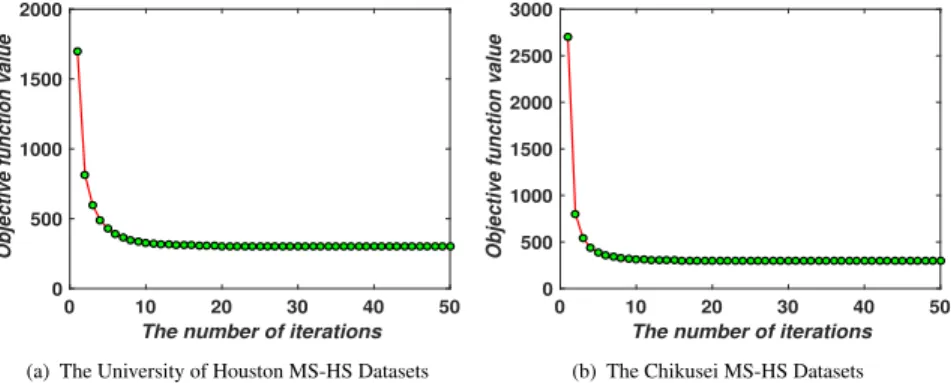
Figure 3: Convergence analysis of LeMA are experimentally performed on the two MS-HS datasets.
ForWfU U, the objective function can be written as 208 min f WU U β 4kWfZk1,1s.t.Wf =Wf T, 1/N kWfi,j0, kWkf 1,1=s, (11)
which can be effectively solved usingAlgorithm 4.
209
Finally, we repeat these optimization procedures until a stopping criterion is
satis-210
fied.
211
2.4. Convergence Analysis
212
The alternative alternating strategy used inAlgorithm 1 is nothing but a block
213
coordinate descent (BCD), which has been theoretically supported to converge to a
214
stationary point as long as each subproblem in Eq. (4) is exactly minimized [35]. As
215
observed, these subproblems with respect to the variablesP,ΘandWf are strongly
216
convex, and hence each independent task can ideally find an unique minimum when the
217
Lagrangian parameter is updated within finitely iterative steps [36]. Besides, ADMM
218
used in each subproblem optimization is actually generalized toinexactAugmented
219
Lagrange Multiplier (ALM) [37], whose convergence has been well studied when the
220
number of block is less than three [38] (e.g.Algorithm 2). Although there is still not a
221
generally and strictlytheoretical proof in multi-blocks case, yet the convergence
anal-222
ysis for some common cases such as ourAlgorithm 3andAlgorithm 4has been well
223
conducted in [39][40][41][42]. We also experimentally record the objective function
values in each iteration to draw the convergence curves of LeMA on two used HS-MS
225
datasets (see Fig. 3).
226
3. Experiments
227
In this section, we quantitatively and qualitatively evaluate the performance of the
228
proposed method on two simulated HS-MS datasets (University of Houston and
Chiku-229
sei) and a real multispectral-lidar and hyperspectral dataset provided by2018IEEE
230
GRSS data fusion contest (DFC2018), by the form of classification using two
com-231
monly used and high-performance classifiers, namely linear support vector machines
232
(LSVM), and canonical correlation forest (CCF) [43]. Three indices: overall accuracy
233
(OA), average accuracy (AA), kappa coefficient (κ), are calculated to quantitatively
234
assess the classification performance. Moreover, we compare the performance of the
235
proposed LeMA and several other state-of-art algorithms, i.e. GLP [31], SMA,
S-236
SMA [29], CoSpace and Semi-supervised CoSpace (S-CoSpace). The original MS
237
data is used as a baseline. SMA constructs an LDA-like joint graph using label
in-238
formation. Besides label information, S-SMA method also uses unlabeled samples to
239
generate the joint graph by computing the similarity based on Euclidean distance. The
240
same strategy of graph construction is adopted for CoSpace and S-CoSpace.
241
3.1. The Simulated MS-HS Datasets over the University of Houston
242
3.1.1. Data Description
243
The HS data in the simulatedHouston MS-HS datasetswas acquired by the
ITRES-244
CASI-1500 sensor with the size of349×1905at a ground sampling distance (GSD) of
245
2.5m over the University of Houston campus and its neighboring urban areas. This data
246
was provided for the2013IEEE GRSS data fusion contest, with 144 bands covering
247
the wavelength range from 364nm to 1046nm. Spectral simulation is performed to
248
generate the MS image by degrading the HS image in the spectral domain using the
249
MS spectral response functions (SRFs) of Sentinel-2 as filters (for more details refer to
250
[6]). The MS data we used is generated with dimensions of349×1905×10.
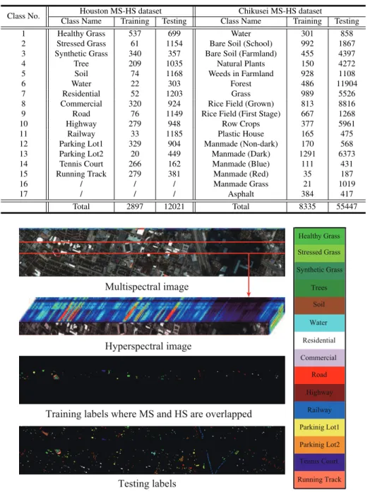
Table 1: The number of training and testing samples for the two used MS-HS datasets.
Class No. Houston MS-HS dataset Chikusei MS-HS dataset
Class Name Training Testing Class Name Training Testing
1 Healthy Grass 537 699 Water 301 858
2 Stressed Grass 61 1154 Bare Soil (School) 992 1867
3 Synthetic Grass 340 357 Bare Soil (Farmland) 455 4397
4 Tree 209 1035 Natural Plants 150 4272
5 Soil 74 1168 Weeds in Farmland 928 1108
6 Water 22 303 Forest 486 11904
7 Residential 52 1203 Grass 989 5526
8 Commercial 320 924 Rice Field (Grown) 813 8816
9 Road 76 1149 Rice Field (First Stage) 667 1268
10 Highway 279 948 Row Crops 377 5961
11 Railway 33 1185 Plastic House 165 475
12 Parking Lot1 329 904 Manmade (Non-dark) 170 568
13 Parking Lot2 20 449 Manmade (Dark) 1291 6373
14 Tennis Court 266 162 Manmade (Blue) 111 431
15 Running Track 279 381 Manmade (Red) 35 187
16 / / / Manmade Grass 21 1019
17 / / / Asphalt 384 417
Total 2897 12021 Total 8335 55447
Multispectral image
Hyperspectral image
Training labels where MS and HS are overlapped
Testing labels Healthy Grass Stressed Grass Synthetic Grass Trees Soil Water Residential Commercial Road Highway Railway Parkinig Lot1 Parkinig Lot2 Tennis Court Running Track
Figure 4: The multispectral image and its corresponding hyperspectral image that partially covers the same area, as well as training and testing labels, for University of Houston dataset.
3.1.2. Experimental Setup
252
To meet our problem setting, a HS image partially overlapping MS image and a
253
whole MS image are used in our experiments, and meanwhile the corresponding
train-254
ing and test samples can be re-assigned, as shown in Fig. 4. In detail, since the total
255
labels are available, we seek out a region where all kinds of classes are involved. The
256
labels in the region are selected as the training set and the rest are seen as the test set,
257
as shown in Fig. 4 and specifically quantified in Table 1.
258
The parameters of the different methods are determined by a 10-fold cross-validation
259
on the training data. More specifically, we tune the parameters of the different
algo-260
rithms to maximize their performances, e.g. dimension (d), penalty parameters (α, β),
261
etc. The dimension (d) is a common parameter for all compared algorithms, and it can
262
be determined covering the range from10to50at an interval of10. For the number
263
of nearest neighbors (k) and the standard deviation of Gaussian kernel function (σ)
264
in artificially computing the adjacency matrix (W) of GLP, SMA, and S-SMA, we
se-265
lect them in the range of{10,20, ...,50}and{10−2,10−1,100,101,102}, respectively,
266
Similarly to CoSpace, S-CoSpace and LeMA, we set the two regularization parameters
267
(α, β) ranging from{10−2,10−1,100,101,102}.
268
3.1.3. Results and Analysis
269
Fig.5 shows the classification maps of compared algorithms using LSVM and CCF
270
classifiers, while Table 2 lists the specific quantitative assessment results with optimal
271
parameters obtained by 10-fold cross-validation.
272
Overall, the methods based on manifold alignment outperform baseline and GLP
273
using the different classifiers. This means that the limited amount of HS data can guide
274
the corresponding MS data towards better discriminative feature representations. More
275
specifically when compared with S-SMA, SMA yields a relatively poor performance
276
since it only considers the correspondences of MS-HS labeled data. This indicates that
277
reasonably embedding unlabeled samples into the manifold alignment framework can
278
effectively help us capture the real data distribution, and thereby obtain more accurate
279
decision boundaries. Unfortunately, these approaches only attempt to align different
280
data in a common subspace, but they hardly take the connections between the common
Baseline L S V M CCF
GLP SMA S-SMA CoSpace S-CoSpace LeMA Training Testing
Healthy Grass Stressed Grass Synthetic Grass Trees Soil Water Residential Commercial Road Highway Railway Parkinig Lot1 Parkinig Lot2 Tennis Court Running Track
Figure 5: Classification maps of the different algorithms obtained using two kinds of classifiers on the University of Houston dataset.
subspace and label information into account2, which leads to a lack of discriminative 282
ability. With regards to this, our proposed joint learning framework “CoSpace” and
283
its semi-supervised version “S-CoSpace” achieve the desired results on the the given
284
MS-HS datasets.
285
By fully considering the connectivity of the common subspace, label information,
286
and unlabeled information encoded by the learned graph structure, the performance
287
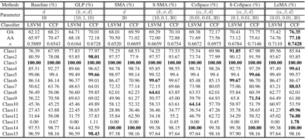
Table 2: Quantitative performance comparison with the different algorithms on the University of Houston data. The best one is shown in bold.
Methods Baseline (%) GLP (%) SMA (%) S-SMA (%) CoSpace (%) S-CoSpace (%) LeMA (%)
Parameter d (k, σ, d) d (k, σ, d) (α, β, d) (α, β, d) (α, β, d) 10 (10,1,10) 30 (10,0.1,30) (0.01,0.01,30) (0.1,0.01,30) (0.01,0.01,30) Classifier LSVM CCF LSVM CCF LSVM CCF LSVM CCF LSVM CCF LSVM CCF LSVM CCF OA 62.12 68.21 64.71 70.01 68.01 69.59 69.29 70.10 69.38 72.17 70.41 73.75 73.42 76.35 AA 65.97 70.47 68.18 72.18 70.50 71.02 72.00 72.88 71.69 73.56 73.12 75.61 74.76 77.18 κ 0.5889 0.6543 0.6164 0.6728 0.6520 0.6695 0.6659 0.6754 0.6672 0.6975 0.6784 0.7146 0.7110 0.7428 Class1 76.39 67.95 77.83 77.97 75.25 68.53 74.25 73.53 75.54 69.96 91.85 87.98 89.56 85.84 Class2 80.59 78.08 93.85 98.01 97.57 77.9 97.57 93.67 73.74 77.99 90.12 91.59 93.67 93.85 Class3 100.00 100.00 100.00 100.00 100.00 100.00 100.00 100.00 100.00 100.00 100.00 100.00 100.00 100.00 Class4 85.51 92.27 89.66 96.62 94.78 98.74 95.85 98.55 98.74 98.26 92.75 97.29 97.49 99.61 Class5 99.06 99.4 99.49 99.66 98.97 99.14 99.32 99.4 99.4 99.4 99.4 99.66 99.49 99.57 Class6 86.14 86.14 96.37 99.01 86.47 70.96 99.67 99.67 85.48 85.15 99.67 96.70 86.47 86.47 Class7 50.62 63.76 48.63 64.01 72.32 77.14 72.15 69.66 73.98 80.05 75.06 80.96 83.21 88.03 Class8 56.49 56.06 56.60 59.85 62.01 62.23 64.61 63.85 63.53 62.01 55.84 60.39 62.77 62.01 Class9 56.22 70.58 69.63 69.02 49.96 61.27 50.57 45.00 59.79 64.93 65.8 71.54 64.49 61.88 Class10 45.36 45.25 45.46 49.89 58.12 52.32 58.33 63.61 64.14 57.70 58.97 51.79 60.97 53.59 Class11 27.43 43.88 22.45 38.65 28.86 36.46 36.46 34.77 36.54 47.26 35.78 38.65 41.27 49.96 Class12 31.64 56.08 31.75 37.83 35.84 62.50 34.18 55.2 46.79 62.72 34.29 58.52 45.02 76.88 Class13 0.00 0.67 0.00 1.11 0.00 0.00 0.00 0.45 0.00 0.45 0.00 0.89 0.00 1.78 Class14 97.53 98.77 94.44 92.59 100.00 100.00 99.38 98.15 100.00 99.38 99.38 100.00 99.38 100.00 Class15 96.59 98.16 96.59 98.43 97.38 98.16 97.64 97.64 97.64 98.16 97.90 98.16 97.64 98.16
of LeMA is much more superior to that of any other methods as can be observed in
288
Table 2. This demonstrates that LeMA is likely to learn a more discriminative feature
289
representation and to find a better decision boundary.
290
As observed from Fig. 4 and Table 2, the training samples are relatively a few and
291
meanwhile the distribution between different classes is extremely unbalanced. While
292
training the classifier, more attentions are paid on those classes with large-size
sam-293
ples, and some small-scale classes possibly play less and even nothing. For this reason,
294
we propose to consider those large-scale unlabeled data, achieving a semi-supervised
295
learning. Using this strategy, the semi-supervised methods, i.e. GLP, SMA,
S-296
CoSpace, obviously perform better than baseline and their supervised ones (SMA and
297
CoSpace). Moreover, we can see from Table 2 that there is a significant improvement of
298
classification performance in some classes (e.g. Stressed Grass,Water) after
account-299
ing for unlabeled samples, particularly between SMA and S-SMA as well as CoSpace
300
and S-CoSpace. However, these aforementioned semi-supervised methods carry out
301
the label propagation on a given graph manually computed by gaussian kernel function,
302
limiting the adaptiveness and discriminability of the algorithms. LeMA can adaptively
303
learn a data-driven graph structure where the labels tend to spread more smoothly,
304
which can result in a more effective material identification for those challenging classes
305
(few training samples), such asTrees,Residential,Railway, Parking Lot1. In
tion, we can also observe an easily overlooked phenomenon that the LeMA’s ability
307
in identifying certain classes still remains limited, such asParking Lot2(only1.78%)
308
andRailway(49.96%). Parking Lot2is basically classified toCommercialand
Park-309
ing Lot1, whileRailwayis largely identified asRoadandCommercial. This might be
310
explained by the limited number of training samples as well as fairly similar spectral
311
properties between several classes.
312
3.2. The Simulated MS-HS Datasets over Chikusei
313
3.2.1. Data Description
314
Similarly to Houston data, the MS data with dimensions of2517×2335×10at a
315
GSD of 2.5 m was simulated by the HS data acquired by the Headwall0s
Hyperspec-316
VNIR-C sensor over Chikusei area, Ibaraki, Japan. It consists of 128 bands in the
317
spectral range from 363nm to 1018nm with the 10nm spectral resolution. The dataset
318
has been made available to the scientific research [44].
319
3.2.2. Experimental Setup
320
Fig. 6 shows the corresponding MS and partial HS images as well as selected
train-321
ing labels and test labels. Again, the overlapped region between MS and HS, which
322
should include all the classes listed in Table 1, is chosen based on the given ground
323
truth [44]. Additionally, the parameters configuration for all algorithms can be
adap-324
tively completed by a 10-fold cross-validation on the training set, which is more
gen-325
eralized to different datasets. Regarding how to run the cross-validation for parameters
326
setting, please refer to section 3.1.2 for more details.
327
3.2.3. Results and Analysis
328
We assess the classification performance of the different algorithms for the
Chiku-329
sei MS-HS data both quantitatively and visually, as shown in Fig.7 and Table 3.
330
Similarly to the University of Houston MS-HS data, there is a basically consistent
331
trend for the different algorithms in the Chikusei MS-HS data. On the whole, the
332
original MS data (baseline) fails to identify some specific materials such asPlastic
333
House,Manmade (Dark),Rice Field (Grown),Bare Soil (Farmland), andForest, due to
Multispectral image
Hyperspectral image
Training labels Testing labels
Water Bare Soil (School) Bare Soil (Farmland)
Natural Plants Weeds in Farmland
Forest Grass Rice Field (Grown) Rice Field (First Stage)
Row Crops Plastic House Manmade (Non-dark) Manmade (Dark) Manmade (Blue) Manmade (Red) Manmade Grass Asphalt
Figure 6: The multispectral image and its corresponding hyperspectral image that partially covers the same area, as well as training and testing labels, for Chikusei Dataset.
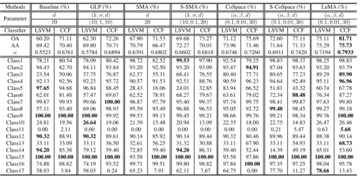
Table 3: Quantitative performance comparison with the different algorithms on the Chikusei data. The best one is shown in bold.
Methods Baseline (%) GLP (%) SMA (%) S-SMA (%) CoSpace (%) S-CoSpace (%) LeMA (%)
Parameter d (k, σ, d) d (k, σ, d) (α, β, d) (α, β, d) (α, β, d) 10 (10,1,10) 20 (10,0.1,20) (0.1,0.01,30) (0.1,0.01,30) (0.1,0.01,30) Classifier LSVM CCF LSVM CCF LSVM CCF LSVM CCF LSVM CCF LSVM CCF LSVM CCF OA 60.20 71.11 62.30 72.26 67.90 71.53 69.68 73.27 71.12 75.69 72.60 77.11 75.11 81.71 AA 69.42 70.40 69.80 70.71 70.79 66.47 72.27 70.01 73.96 71.46 71.64 71.33 75.29 75.73 κ 0.5523 0.6761 0.5784 0.6894 0.6391 0.6802 0.6602 0.6818 0.6746 0.7260 0.6911 0.7420 0.7194 0.7933 Class1 78.21 80.54 78.09 80.42 98.72 82.52 99.53 97.90 92.54 79.25 98.83 98.37 98.25 98.83 Class2 94.43 82.70 94.11 93.84 93.20 92.50 93.20 93.09 93.47 94.91 87.04 93.63 93.20 93.79 Class3 23.54 50.06 37.75 76.87 62.57 55.31 68.41 76.55 80.40 77.71 80.65 77.23 89.29 89.90 Class4 92.13 92.56 92.23 95.72 90.57 91.53 92.51 88.76 90.59 96.23 94.64 92.49 95.11 96.96 Class5 97.65 94.68 96.84 88.45 28.43 16.06 24.01 32.85 83.94 66.52 51.81 43.32 60.74 67.78 Class6 62.01 81.48 57.47 69.67 62.52 78.91 68.27 79.67 63.61 79.02 72.34 88.48 76.34 87.27 Class7 99.67 99.93 99.66 100.00 96.87 97.79 95.40 99.37 97.74 99.75 98.41 99.87 97.63 99.80 Class8 57.11 93.40 69.06 98.93 95.59 93.49 96.88 96.53 95.05 92.72 99.48 98.45 99.27 99.18 Class9 100.00 100.00 100.00 99.92 99.53 99.13 99.45 99.21 98.66 99.76 99.21 98.34 99.76 100.00 Class10 24.81 19.56 26.64 19.06 21.39 15.48 20.94 13.09 22.35 18.00 22.75 14.83 26.47 26.46 Class11 0.00 2.11 0.00 0.00 0.00 0.00 0.00 0.00 0.00 0.00 0.21 5.47 0.63 5.68 Class12 90.32 88.91 90.32 89.61 90.14 85.92 90.14 89.44 90.32 80.46 89.96 89.44 88.38 90.14 Class13 33.11 33.09 33.11 36.50 32.61 56.25 31.32 30.88 33.11 67.90 33.11 54.93 33.11 68.73 Class14 94.20 85.38 79.12 59.40 72.85 59.40 94.20 86.31 59.40 52.44 14.39 49.19 45.01 53.60 Class15 100.00 100.00 100.00 100.00 93.58 100.00 100.00 100.00 93.58 97.86 100.00 100.00 100.00 100.00 Class16 74.88 88.62 74.19 93.52 99.71 99.51 99.80 98.82 97.84 100.00 97.35 97.25 98.04 95.78 Class17 58.03 3.84 58.03 0.24 65.23 7.91 62.11 7.67 64.75 0.00 77.70 11.27 78.66 13.43
L S V M CCF Baseline GLP
SMA S-SMA CoSpace S-CoSpace LeMA
SMA S-SMA CoSpace S-CoSpace LeMA Baseline GLP Water
Bare Soil (School) Bare Soil (Farmland)
Natural Plants Weeds in Farmland
Forest
Grass Rice Field (Grown) Rice Field (First Stage)
Row Crops Plastic House Manmade (Non-dark) Manmade (Dark) Manmade (Blue) Manmade (Red) Manmade Grass Asphalt RGB Training Testing
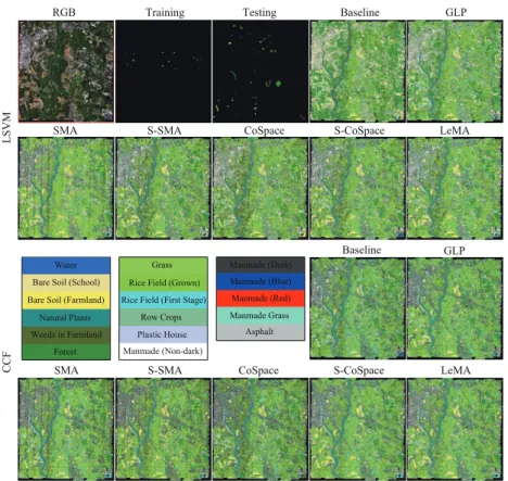
Figure 7: Classification maps of the different algorithms obtained using two kinds of classifiers on the Chikusei dataset.
its poor spectral information and a limited number of training samples. GLP utilizes the
335
unlabeled samples to augment the training samples in a semi-supervised way, yet it is
336
still limited by the low-discriminative spectral signatures. By aligning the MS and HS
337
data, these alignment-based approaches (e.g. SMA, S-SMA, CoSpace, S-CoSpace, and
338
LeMA) are able to find a common subspace in which the learnt features are expected to
339
absorb the different properties from two modalities, resulting in a better performance.
340
Compared to the supervised methods (SMA and CoSpace), their corresponding
semi-341
supervised versions (S-SMA and S-CoSpace) obtain higher classification accuracies
342
on both classifiers, which is detailed in Table 3. As expected, the performance of
343
the LeMA is significantly superior to that of others, thanks to the great contributions
344
of a common subspace learning from MS-HS data, a data-driven graph learning and
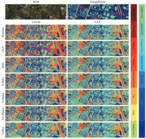
Ba se li ne LSVM CCF G L P S M A S -S M A CoS pa ce S -CoS pa ce L eM A RGB GroundTruth H ea lthy G ra ss St re ss ed G rass E ve rgre e n T re e s D ec id uou s T ree s Bare E ar th Resi de n tial N on -resi de n tial Ro ads Si d ew al ks M aj or Thor oug hfare s H ighw ay s Rai lw ay s Pave d P ark ing L ot s Cars T ra ins St adi um Sea ts
Figure 8: Classification maps of the different algorithms obtained using two kinds of classifiers on the real dataset of DFC2018 (Multispectral-Lidar and Hyperspectral data).
the semi-supervised learning strategy. Despite so, the LeMA still fails to recognize
346
some challenging classes, such asWeeds in Farmland,Row Crops,Plastic House, and
347
Asphalt. The reasons could be two-fold. On one hand, the performance of LeMA
348
is limited, to some extent, by the unbalanced data sets. On the other hand, LeMA’
349
transferring ability would sharply degrade when a great spectral variability between
350
training and test samples exists.
351
3.3. The Real Multispectral-Lidar and Hyperspectral Datasets in DFC2018
352
Although we follow strict simulation procedures, yet the two MS-HS datasets used
353
above (Houston and Chikusei) essentially originate from a similar data source
(ho-354
mogeneous), which means there is a strong correlation in their spectral features. This
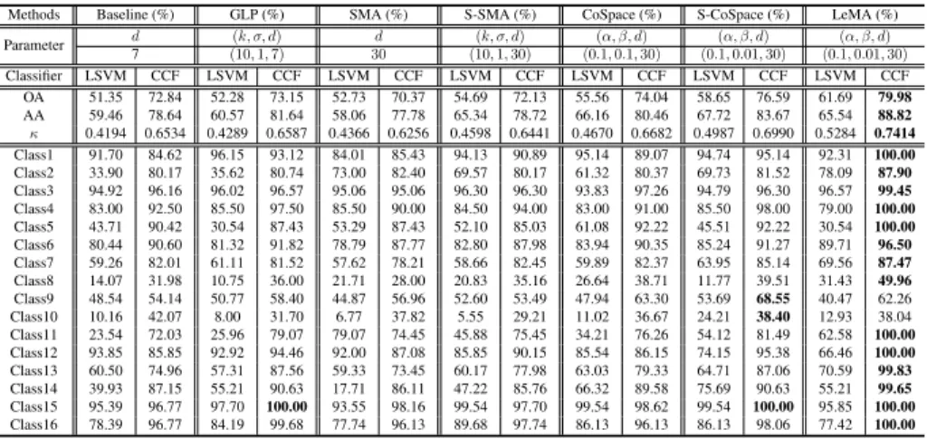
Table 4: Quantitative performance comparison with the different algorithms on the DFC2018 data. The best one is shown in bold.
Methods Baseline (%) GLP (%) SMA (%) S-SMA (%) CoSpace (%) S-CoSpace (%) LeMA (%)
Parameter d (k, σ, d) d (k, σ, d) (α, β, d) (α, β, d) (α, β, d) 7 (10,1,7) 30 (10,1,30) (0.1,0.1,30) (0.1,0.01,30) (0.1,0.01,30) Classifier LSVM CCF LSVM CCF LSVM CCF LSVM CCF LSVM CCF LSVM CCF LSVM CCF OA 51.35 72.84 52.28 73.15 52.73 70.37 54.69 72.13 55.56 74.04 58.65 76.59 61.69 79.98 AA 59.46 78.64 60.57 81.64 58.06 77.78 65.34 78.72 66.16 80.46 67.72 83.67 65.54 88.82 κ 0.4194 0.6534 0.4289 0.6587 0.4366 0.6256 0.4598 0.6441 0.4670 0.6682 0.4987 0.6990 0.5284 0.7414 Class1 91.70 84.62 96.15 93.12 84.01 85.43 94.13 90.89 95.14 89.07 94.74 95.14 92.31 100.00 Class2 33.90 80.17 35.62 80.74 73.00 82.40 69.57 80.17 61.32 80.37 69.73 81.52 78.09 87.90 Class3 94.92 96.16 96.02 96.57 95.06 95.06 96.30 96.30 93.83 97.26 94.79 96.30 96.57 99.45 Class4 83.00 92.50 85.50 97.50 85.50 90.00 84.50 94.00 83.00 91.00 85.50 98.00 79.00 100.00 Class5 43.71 90.42 30.54 87.43 53.29 87.43 52.10 85.03 61.08 92.22 45.51 92.22 30.54 100.00 Class6 80.44 90.60 81.32 91.82 78.79 87.77 82.80 87.98 83.94 90.35 85.24 91.27 89.71 96.50 Class7 59.26 82.01 61.11 81.52 57.62 78.21 58.66 82.45 59.89 82.37 63.95 85.14 69.56 87.47 Class8 14.07 31.98 10.75 36.00 21.71 28.00 20.83 35.16 26.64 38.71 11.77 39.51 31.43 49.96 Class9 48.54 54.14 50.77 58.40 44.87 56.96 52.60 53.49 47.94 63.30 53.69 68.55 40.47 62.26 Class10 10.16 42.07 8.00 31.70 6.77 37.82 5.55 29.21 11.02 36.67 24.21 38.40 12.93 38.04 Class11 23.54 72.03 25.96 79.07 79.07 74.45 45.88 75.45 34.21 76.26 54.12 81.49 62.58 100.00 Class12 93.85 85.85 92.92 94.46 92.00 87.08 85.85 90.15 85.54 86.15 74.15 95.38 66.46 100.00 Class13 60.50 74.96 57.31 87.56 59.33 73.45 60.17 77.98 63.03 79.33 64.71 87.06 70.59 99.83 Class14 39.93 87.15 55.21 90.63 17.71 86.11 47.22 85.76 66.32 89.58 75.69 90.63 55.21 99.65 Class15 95.39 96.77 97.70 100.00 93.55 98.16 99.54 97.70 99.54 98.62 99.54 100.00 95.85 100.00 Class16 78.39 96.77 84.19 99.68 77.74 96.13 89.68 97.74 86.13 96.13 86.13 98.06 77.42 100.00
makes the information of the different modalities transferred more effectively, but could
356
limit the generalization ability in practice. To this end, we apply a real bi-modal dataset
357
– multispectral-lidar and hyperspectral (heterogeneous) provided by the latest IEEE
358
GRSS data fusion contest 2018 (DFC2018).
359
3.3.1. Data Description
360
Multi-source optical remote sensing data, such as multispectral-lidar data,
hyper-361
spectral data, and very high-resolution RGB data, is provided in the contest. More
362
specifically, the multispectral-lidar imagery consists of1202×4768pixels with 7 bands
363
( 3 intensity bands and 4 DSMs-related bands [45]) collected from 1550nm, 1064nm,
364
and 532nm at a 0.5m GSD, while the hyperspectral data comprises 48 bands covering
365
a spectral range from 380nm to 1050nm at 1m GSD, and its size is601×2384. In
366
our case, our LeMA model is trained on partial multispectral-lidar and hyperspectral
367
correspondences and tested only using multispectral-lidar data, in order to meet the
368
requirement of our cross-modality learning task. The first row of Fig.8 shows the RGB
369
image of this scene and the labeled ground truth image.
370
3.3.2. Experimental Setup
371
Our aim is, once again, to investigate whether the limited amount of hyperspectral
372
data can improve the performance of another modality, e.g., multispectral data
geneous) or multispectral-lidar data (heterogeneous). Therefore, we randomly assign
374
10% of total labeled samples as training set and the rest of it as test set in the
ex-375
periment. Moreover, 16 main classes are selected out of 20 (see Fig.8), by removing
376
several small classes with too few samples, e.g. Artificial Turf,Water,Crosswalks,
377
andUnpaved Parking Lots. Likewise, we automatically configure the parameters of
378
the proposed LeMA and the compared algorithms by a 10-fold cross-validation on the
379
training set, which is detailed in section 3.1.2.
380
3.3.3. Results and Analysis
381
We show the averaged results of the different algorithms out of 10 runs to obtain
382
a relatively stable and meaningful performance comparison, because the training and
383
test sets are randomly generated from total samples in each round, as listed in Table 4.
384
Correspondingly, Fig. 8 visually highlights the differences of classification maps for
385
the different methods.
386
Generally speaking, hyperspectral information embedding can effectively improve
387
the classification performance of the multispectral-lidar data, which implies that the
388
models based common subspace learning (e.g., SMA, S-SMA, CoSpace, S-CoSpace,
389
and LeMA) can transfer the knowledge from one modality to another modality to some
390
extent. We also observe from Table 4 that the semi-supervised methods which consider
391
the unlabeled samples (e.g., GLP, S-SMA, S-CoSpace, and LeMA) always perform
392
better than those purely supervised ones. Not unexpectedly, LeMA integrating rich
393
spectral information and unlabeled samples achieves a superior performance, which
394
demonstrates that the learning-based graph structure is more applicable to capturing
395
the data distribution and further find a potential optimal decision boundary.
396
One thing to be noted, however, is that compared to the performance of the different
397
algorithms in the simulated MS-HS datasets from similar sources (homogeneous), the
398
knowledge transferring ability of these algorithms in handling the real
multispectral-399
lidar and hyperspectral datasets from different sources (heterogeneous) remains
lim-400
ited, since all listed methods including our LeMA are modeled in a linearized way.
401
Unfortunately, a single linear transformation fails to fit the gap between heterogeneous
402
modalities well, despite a limited performance improvement.
4. Conclusions
404
In real-world problems, a large amount of low-quality data (e.g. MS data) can
405
often be easily collected. On the contrary, high-quality data (e.g. HS data) are
usu-406
ally expensive and difficult to obtain. This motivates us to investigate whether a
lim-407
ited amount of high-quality data can contribute to relevant tasks with a large amount
408
of low-quality data. For this purpose, we propose a novel semi-supervised learning
409
framework called LeMA, which effectively connects the common subspace and label
410
information, and automatically embeds the unlabeled information into the proposed
411
framework by adaptively learning a Laplacian matrix from the data. Extensive
exper-412
iments are conducted using the LeMA on two homologous MS-HS simulated datasets
413
and a heterogenous multispectral-lidar and hyperspectral real dataset in comparison
414
with the other state-of-arts algorithms, demonstrating the superiority and effectiveness
415
of the LeMA in the knowledge transferring ability. We have to admit, however, that
de-416
spite a significant performance improvement in LeMA, yet its representative ability is
417
still limited by linearly modeling way, especially facing highly-nonlinear heterogenous
418
data. Towards this issue, we will continue to improve our model to a nonlinear version
419
and simultaneously consider the spatial information (e.g., morphological profiles) to
420
further strengthen the feature representation ability.
421
5. Acknowledgements
422
The authors would like to thank the Hyperspectral Image Analysis group and the
423
NSF Funded Center for Airborne Laser Mapping (NCALM) at the University of
Hous-424
ton for providing the CASI University of Houston dataset. The authors would like to
425
express their appreciation to Prof. D. Cai and Dr. C. Wang for providing MATLAB
426
codes for LPP and manifold alignment algorithms.
427
This work was supported by funding from the European Research Council (ERC)
428
under the European Union’s Horizon 2020 research and innovation program (grant
429
agreement No [ERC-2016-StG-714087]) and from Helmholtz Association under the
430
framework of the Young Investigators Group ”SiPEO” (VH-NG-1018, www.sipeo.bgu.
431
tum.de). The work of N. Yokoya was supported by Japan Society for the Promotion
of Science (JSPS) KAKENHI 15K20955 and Alexander von Humboldt Fellowship for
433
postdoctoral researchers.
434
[1] X. Huang, Q. Lu, L. Zhang, A multi-index learning approach for classification of
435
high-resolution remotely sensed images over urban areas, ISPRS J.
Photogram-436
metry Remote Sens. 90 (2014) 36–48.
437
[2] D. Hong, N. Yokoya, X. Zhu, The k-lle algorithm for nonlinear dimensionality
438
ruduction of large-scale hyperspectral data, in: Hyperspectral Image and Signal
439
Processing: Evolution in Remote Sensing (WHISPERS), 2016 8th Workshop on,
440
IEEE, 2016, pp. 1–5.
441
[3] J. Kang, M. K¨orner, Y. Wang, H. Taubenb¨ock, X. Zhu, Building instance
classifi-442
cation using street view images, ISPRS J. Photogrammetry Remote Sens.
443
[4] C. Yang, J. H. Everitt, Q. Du, B. Luo, J. Chanussot, Using high-resolution
air-444
borne and satellite imagery to assess crop growth and yield variability for
preci-445
sion agriculture, Proc. IEEE 101 (3) (2013) 582–592.
446
[5] F. D. V. der Meer, H. M. A. V. der Werff, F. J. A. V. Ruitenbeek, Potential of
447
esa’s sentinel-2 for geological applications, Remote Sens. Environ. 148 (2014)
448
124–133.
449
[6] N. Yokoya, C. Grohnfeldt, J. Chanussot, Hyperspectral and multispectral data
450
fusion: a comparative review, IEEE Geosci. Remote Sens. Mag. 5 (2) (2017)
451
29–56.
452
[7] D. Hong, N. Yokoya, X. Zhu, Learning a robust local manifold representation for
453
hyperspectral dimensionality reduction, IEEE J. Sel. Topics Appl. Earth Observ.
454
Remote Sens. 10 (6) (2017) 2960–2975.
455
[8] J. Li, H. Zhang, L. Zhang, Column-generation kernel nonlocal joint collaborative
456
representation for hyperspectral image classification, ISPRS J. Photogrammetry
457
Remote Sens. 94 (2014) 25–36.
[9] Y. Tarabalka, J. Benediktsson, J. Chanussot, Spectral-spatial classification of
459
hyperspectral imagery based on partitional clustering techniques, IEEE Trans.
460
Geosci. Remote Sens. 47 (8) (2009) 2973–2987.
461
[10] L. Zhang, L. Zhang, D. Tao, X. Huang, On combining multiple features for
hyper-462
spectral remote sensing image classification, IEEE Trans. Geosci. Remote Sens.
463
50 (3) (2012) 879–893.
464
[11] D. Hong, N. Yokoya, J. Xu, X. Zhu, Joint and progressive learning from
high-465
dimensional data for multi-label classification, in: European Conference on
Com-466
puter Vision (ECCV), Springer, 2018, pp. 478–493.
467
[12] J. Xia, J. Chanussot, P. Du, X. He, Semi-supervised probabilistic principal
com-468
ponent analysis for hyperspectral remote sensing image classification, IEEE J.
469
Sel. Topics Appl. Earth Observ. Remote Sens. 7 (6) (2014) 2224–2236.
470
[13] D. Tuia, M. Volpi, M. Trolliet, G. Camps-Valls., Semisupervised manifold
align-471
ment of multimodal remote sensing images, IEEE Trans. Geosci. Remote Sens.
472
52 (12) (2014) 7708–7720.
473
[14] L. Bruzzone, M. Marconcini, Domain adaptation problems: A dasvm
classifica-474
tion technique and a circular validation strategy, IEEE Trans. Pattern Anal. Mach.
475
Intell. 32 (5) (2010) 770–787.
476
[15] B. Banerjee, F. Bovolo, A. Bhattacharya, L. Bruzzone, S. Chaudhuri, K. M.
Bud-477
dhiraju, A novel graph-matching-based approach for domain adaptation in
classi-478
fication of remote sensing image pair, IEEE Trans. Geosci. Remote Sens. 53 (7)
479
(2015) 4045–4062.
480
[16] G. Matasci, M. Volpi, M. Kanevski, L. Bruzzone, D. Tuia, Semisupervised
trans-481
fer component analysis for domain adaptation in remote sensing image
classifi-482
cation, IEEE Trans. Geosci. Remote Sens. 53 (7) (2015) 3550–3564.
483
[17] D.Tuia, C. Persello, L. Bruzzone, Domain adaptation for the classification of
re-484
mote sensing data: An overview of recent advances, IEEE Geosci. Remote Sens.
485
Mag. 4 (2) (2016) 41–57.
[18] A. Samat, P. Gamba, J. Abuduwaili, S. Liu, Z. Miao, Geodesic flow kernel support
487
vector machine for hyperspectral image classification by unsupervised subspace
488
feature transfer, Remote Sens. 8 (3) (2016) 234.
489
[19] A. Samat, C. Persello, P. Gamba, S. Liu, J. Abuduwaili, E. Li, Supervised and
490
semi-supervised multi-view canonical correlation analysis ensemble for
hetero-491
geneous domain adaptation in remote sensing image classification, Remote Sens.
492
9 (4) (2017) 337.
493
[20] A. Khosla, T. Zhou, T. Malisiewicz, A. Efros, A. Torralba, Undoing the damage
494
of dataset bias, in: European Conference on Computer Vision (ECCV), Springer,
495
2012, pp. 158–171.
496
[21] C. Woodcock, S. A. Macomber, M. Pax-Lenney, W. B. Cohen, Monitoring large
497
areas for forest change using landsat: Generalization across space, time and
land-498
sat sensors, Remote Sens. Environ. 78 (1-2) (2001) 194–203.
499
[22] J. Jiang, X. Zhai, Instance weighting for domain adaptation in nlp, in:
Proceed-500
ings of ACL, 2007, pp. 264–271.
501
[23] M. Sugiyama, S. Nakajima, H. Kashima, P. Buenau, M. Kawanabe, Direct
im-502
portance estimation with model selection and its application to covariate shift
503
adaptation, in: Advances in neural information processing systems (NIPS), 2008,
504
pp. 1433–1440.
505
[24] A. Samat, P. Gamba, S. Liu, P. Du, J. Abuduwaili, Jointly informative and
man-506
ifold structure representative sampling based active learning for remote sensing
507
image classification, IEEE Trans. Geosci. Remote Sens. 54 (11) (2016) 6803–
508
6817.
509
[25] C. C. Persello, L. Bruzzone, Active learning for domain adaptation in the
super-510
vised classification of remote sensing images, IEEE Trans. Geosci. Remote Sens.
511
50 (11) (2012) 4468–4483.
512
[26] C. Wang, P. Krafft, S. Mahadevan, Chapter of Manifold Learning: Theory and
513
Applications-Manifold alignment, CSC Press, 2011.
[27] D. Tuia, D. Marcos, G. Camps-Valls, Multi-temporal and multi-source remote
515
sensing image classification by nonlinear relative normalization, ISPRS J.
Pho-516
togrammetry Remote Sens. 120 (2016) 1–12.
517
[28] D. Liao, Y. Qian, J. Zhou, Y. Tang, A manifold alignment approach for
hyperspec-518
tral image visualization with natural color, IEEE Trans. Geosci. Remote Sens.
519
54 (6) (2016) 3151–3162.
520
[29] C. Wang, S. Mahadevan, A general framework for manifold alignment, in: AAAI
521
Fall Symposium on Manifold Learning and its Applications (AAAI), 2009.
522
[30] C. Wang, S. Mahadevan, Heterogeneous domain adaptation using manifold
align-523
ment, in: Proceedings of the 22th International Joint Conference on Artificial
524
Intelligence (IJCAI), 2011, pp. 1541–1546.
525
[31] X. Zhu, Z. Ghahramani, J. D. Lafferty, Semi-supervised learning using gaussian
526
fields and harmonic functions, in: Proceedings of the 20th International
Confer-527
ence on Machine learning (ICML), 2003, pp. 912–919.
528
[32] S. Ji, J. Ye, Linear dimensionality reduction for multi-label classification, in:
Pro-529
ceedings of the 21th International Joint Conference on Artificial Intelligence
(IJ-530
CAI), 2009, pp. 1077–1082.
531
[33] Q. Gu, Z. Li, J. Han, Joint feature selection and subspace learning, in:
Proceed-532
ings of the 22th International Joint Conference on Artificial Intelligence (IJCAI),
533
2011, pp. 1294–1299.
534
[34] F. Heide, W. Heidrich, G. Wetzstein, Fast and flexible convolutional sparse
cod-535
ing, in: IEEE Conference on Computer Vision and Pattern Recognition (CVPR),
536
2015, pp. 5135–5143.
537
[35] D. P. Bertsekas, Nonlinear programming, Athena scientific Belmont, 1999.
538
[36] S. Boyd, N. Parikh, E. Chu, B. Peleato, J. Eckstein, Distributed optimization and
539
statistical learning via the alternating direction method of multipliers,
Founda-540
tions and TrendsR in Machine learning 3 (1) (2011) 1–122. 541
[37] L. Chen, X. Li, D. Sun, K. Toh, On the equivalence of inexact proximal
542
alm and admm for a class of convex composite programming, arXiv preprint
543
arXiv:1803.10803.
544
[38] Z. Lin, M. Chen, Y. Ma, The augmented lagrange multiplier method for exact
545
recovery of corrupted low-rank matrices, arXiv preprint arXiv:1009.5055.
546
[39] D. Hong, N. Yokoya, J. Chanussot, X. Zhu, Learning low-coherence dictionary to
547
address spectral variability for hyperspectral unmixing, in: Proceedings of IEEE
548
International Conference on Image Processing (ICIP), 2017, pp. 1–5.
549
[40] G. Liu, Z. Lin, S. Yan, J. Sun, Y. Yu, Y. Ma, Robust recovery of subspace
struc-550
tures by low-rank representation, IEEE Trans. Pattern Anal. Mach. Intell. 35 (1)
551
(2013) 171–184.
552
[41] Y. Zhong, X. Wang, L. Zhao, R. Feng, L. Zhang, Y. Xu, Blind spectral unmixing
553
based on sparse component analysis for hyperspectral remote sensing imagery,
554
ISPRS J. Photogrammetry Remote Sens. 119 (2016) 49–63.
555
[42] P. Zhou, C. Zhang, Z. Lin, Bilevel model based discriminative dictionary learning
556
for recognition, IEEE Trans. Image Process. 26 (3) (2017) 1173–1187.
557
[43] R. Tom, W.Frank, Canonical correlation forests, arXiv preprint
558
arXiv:1507.05444.
559
[44] N. Yokoya, A. Iwasaki, Airborne hyperspectral data over chikusei, Tech. Rep.
560
SAL-2016-05-27.
561
[45] B. L. Saux, N. Yokoya, R. Hansch, S. Prasad, 2018 ieee grss data fusion contest:
562
Multimodal land use classification [technical committees], IEEE Geosci. Remote
563
Sens. Mag. 6 (1) (2018) 52–54.