E
CONOMIC
C
OMMENTARY
Number 2010-14 October 19, 2010Out of the Shadows: Projected Levels
for Future REO Inventory
Guhan Venkatu
Nearly one homeowner in ten is more than 90 days delinquent on his mortgage payment. Most of the homes under these mortgages are likely to be repossessed by lenders and resold, which has led some to call them a shadow inventory. How much these homes will affect the broader housing market depends on when they actually become available for sale and how long they remain on the market. Some analysts are concerned that a surge in the availability of repossessed or real-estate owned (REO) properties, or a persistently high level of them, could put downward pressure on prices. This could, in turn, induce additional foreclosures. This Commentary presents three possible scenarios for future REO inventory levels.
ISSN 0428-1276
Figure 1. Current Stock of Seriously
Delinquent Loans
Source: Mortgage Bankers Association.
0 0.5 1.0 1.5 2.0 2.5 3.0 3.5 4.0 4.5 2000 2001 2002 2003 2004 2005 2006 2007 2008 2009 2010 Millions of homes Foreclosure inventory 90+ day-delinquent inventory
According to the most recent estimates from the Mortgage Bankers Association, approximately 4.1 million borrow-ers are in foreclosure or near it, the latter being borrowborrow-ers who are more than 90 days delinquent on their mortgages (see fi gure 1). Together, these two groups of borrowers are sometimes called “seriously delinquent.” Both in absolute terms and as a proportion of outstanding mortgages, seri-ous delinquencies remain near record highs.
Because a large fraction of these borrowers are also expected to have to leave their homes—either through the foreclosure process or some other distressed exit—observ-ers have referred to this stock of homes as a “shadow inventory.” This inventory, it is feared, will soon fl ow onto the market, drive down prices further, and perhaps cause another wave of defaults.
One crude way of appreciating the size of this inventory is to translate it into the number of months it will likely take to sell this stock. At the current sales pace, the actual inven-tory of existing homes for sale would take about 11 months to work through. Adding in the shadow inventory—which is about the same size as the actual inventory—roughly doubles the time to just under two years. Not surprisingly, this is well above historical averages.
The shadow inventory has already had a signifi cant impact on the composition of recent sales. RealtyTrac, a private company that tracks foreclosures, has reported that roughly one-quarter to one-third of the sales in the fi rst half of 2010 were associated with a home in some stage
of foreclosure. This includes homes that have been repos-sessed by banks or investors after a foreclosure, so-called real-estate owned (REO) properties, which accounted for just under two-thirds of these distressed sales. Distressed properties sold for 26 to 27 percent less than their non-distressed counterparts. Aside from keeping downward pressure on prices, the shadow inventory has also limited new construction—new homes available for sale are at their lowest levels since the late 1960s.
What can we expect going forward? This Commentary
projects how the current shadow inventory could trans-late into actual inventory, as properties move through the foreclosure process to become REOs. These projections show that even with fairly benign assumptions about the likely fl ow of loans into serious delinquency, and under various plausible assumptions about how the foreclosure and pre-foreclosure processes might change, the stock of REO properties is likely to remain elevated for the next several years. This should keep downward pressure on prices, though another factor infl uencing prices is how much deterioration properties suffer during lengthy pre-REO processes.
Transition and Retention Rates
Until recently, the number of borrowers in foreclosure or more than 90 days delinquent was fairly stable, since the number of loans entering these categories was generally being balanced by the number of loans leaving them. But that balance has been affected by recent developments. The rising stock of seriously delinquent loans means that the fl ows into and out of foreclosure and 90+ day delin-quency have changed in an appreciable way. Figure 1 sug-gests that the number of loans fl owing into these categories is exceeding the number of loans fl owing out of them. What’s less clear, however, is how the fl ows themselves are changing. Understanding the way these fl ows are changing is critical, since these changes will ultimately determine the timing and number of REO properties that emerge. Data from LPS Applied Analytics allow us to track the move-ments of loans through the process outlined in fi gure 2, and determine the rates at which loans are transitioning from one state to another.
Figure 3 shows how these fl ows have changed recently with respect to the 90+ day delinquency category. The fl ows are measured as the proportion of loans in a given category that move to some other state (transition rate) or remain in the same state (retention rate). From fi gure 3, we can see a sharp increase in the proportion of loans that don’t transition out of 90+ day delinquency. The
proportion rises from between 70 percent to 75 percent retention to around 85 percent retention more recently. This increase occurs toward the end of 2008, a change that could be consistent with rising bankruptcies and increas-ing attempts to modify troubled mortgages, both of which would delay an impending foreclosure. This explanation is also consistent with what we see in the movement of loans from 90+ day delinquency to foreclosure. That propor-tion falls at about the same time, and by approximately the same amount.
A similar pattern is apparent with the foreclosure stock, though the timing differs. Prior to 2007, between 70 percent and 75 percent of loans in foreclosure in a given month re-mained there the following month. More recently, however, a far greater proportion of foreclosures have survived to the following month—typically more than 85 percent.
The timing of this increase coincides with the fl ood of foreclosures that began in late 2006. It could be that the sharp increase in new foreclosures overwhelmed the courts and other administrative foreclosure processes, decreas-ing the disposition rate. However, it could also be the case that each individual foreclosure is taking about the same amount of time to work through the foreclosure process as before, but that there are simply more foreclosures that are in the early stages of this process. This compositional change would also generate the pattern that we observe in the data. Evidence from other sources suggests that both are in fact occurring.
The fact that a smaller proportion of loans are leaving foreclosure every month also means, of course, that a smaller proportion are transitioning to other states. Nota-bly, prior to 2009, about 8 percent of loans in foreclosure were transitioning to REO properties. That proportion has been halved more recently.
Figures 3 and 4 only show data associated with some of the fl ows illustrated in fi gure 2. However, we will use infor-mation associated with all of the fl ows shown in fi gure 2 to estimate how quickly the current stock of seriously delin-quent loans will likely move through the system.
Figure 2. Delinquency and Foreclosure Flows
90+ days
delinquent Foreclosure REO
To current or paid off
To liquidation
To less serious states of delinquency
From less serious states of delinquency
Figure 3. Monthly Transition and Retention
Rates for 90+ Day Delinquency Stock
Source: LPS Applied Analytics.
Note: Rates shown are 3-month moving averages.
Figure 4. Monthly Transition and
Reten-tion Rates for Foreclosure Stock
Source: LPS Applied Analytics.
Note: Rates shown are 3-month moving averages.
5 10 15 20 Percent 65 70 75 80 85 Percent 2005 2006 2007 2008 2009 2010 Retained Transitioning to foreclosure 4 6 8 10 Percent 70 75 80 85 90 Percent 2005 2006 2007 2008 2009 2010 Retained Transitioning to REO REO Stock Projections
Using alternative assumptions about retention and tran-sition rates, I simulate three different scenarios for the growth path of the REO stock. All three scenarios share some assumptions, including how many new loans will fl ow into serious delinquency over the course of the simu-lation, how many properties will be sold out of REO each period, and how large the current REO inventory is. The number of loans that are likely to fl ow into serious delinquency over the course of the simulation is based on recent history. According to data from LPS, the number of loans transitioning to 90-day delinquency from 60-day delinquency averaged about 50,000 per month from 2005 to the fi rst quarter of 2007. These fl ows then rose sharply, averaging about 200,000 throughout 2009, before falling markedly in 2010 to about 150,000 by mid-year. I assume that these fl ows decline in even increments over the projec-tion period from 150,000 loans to the levels that prevailed from 2005 to early 2007. This assumption generates a relatively slow decline in this fl ow, which is consistent with earlier regional housing booms and busts, where delin-quencies and foreclosure starts remained elevated for years after having peaked.
For REO liquidation rates, I estimate from the data that about 15 percent of each month’s REO inventory is sold. This corresponds to an average REO timeline of just over 6½ months, and would include the time needed for repairs or other work to make the property marketable.
Finally, several sources have estimated the current REO inventory to be about a half-million homes. I use this as the starting size of the REO stock.
Scenario 1: Transition and retention rates remain essentially unchanged
For the fi rst scenario simulated, transition and retention rates remain essentially as they are currently.
Under the full set of assumptions, the REO stock rises modestly, and then drifts gradually downward to just below 350,000 by the end of the third year (fi gure 5). At this point, about 2.8 million loans will have transitioned to REO; 2.3 million loans will remain in a state of serious delinquency; and about 3.0 million loans will have exited the system by permanently transitioning to a less serious state of delinquency, becoming current, or paying off. Scenario 2: Increase in transition rate from 90+ day delinquency to foreclosure
For a few reasons related to the federal government’s mort-gage modifi cation efforts, we might expect the transition rate associated with the movement of loans from 90+ day delinquency to foreclosure to increase soon. The Home Affordable Mortgage Program (HAMP) is the federal government’s primary mortgage modifi cation initiative. Modifi cations initiated through it generally involve a three-month trial phase, which if completed successfully, should result in a permanent modifi cation. As a consequence, the program has had an infl uence on delinquency timelines, slowing the transition to foreclosure, but this is likely to diminish soon for the following reasons.
First, the number of new trial modifi cations being started has slowed substantially in recent months. In the second half of 2009, new trials were being initiated at a monthly rate of about 130,000. That fi gure has fallen by more than half, to roughly 55,000, for the fi rst six months of 2010.
Moreover, in July and August, the average was about 17,000 trials started. It seems likely that the number of new trials will continue to diminish.
Second, most of the trials that have been started have not transitioned to permanent modifi cations. The roughly 660,000 borrowers who were unable to successfully com-plete their trial modifi cations, and for whom foreclosure had been held off, are likely to transition to foreclosure soon. Finally, the number of active trial modifi cations has fallen from just over 450,000 in May to just over 200,000 in August. As fewer borrowers are in active trial modifi ca-tions, a larger proportion of 90+ day delinquencies will be transitioning to foreclosure; put another way, the transition rate from 90+ day delinquency to foreclosure will rise. In the second scenario simulated, I assume that this transi-tion rate rises to 20 percent, close to the levels seen toward the latter part of 2007 and in early 2008, from 7 percent in the initial simulation. (Outside of a smaller proportion of 90+ day delinquencies being retained as a result of this change, all other rates in the initial simulation remain unchanged.) Because the transition rate from 90+ day delinquency to foreclosure increases while the transition rate from foreclosure to REO stays the same, the initial impact is a build-up in the foreclosure stock (fi gure 5). This is associated with an increase in the number of properties moving to the REO stage. As long as this fl ow into REO exceeds the fl ow out from liquidations, the REO stock will build. This is exactly what we observe in the simulated path until July 2011.
The REO stock rises gradually until peaking in mid-2011 at about 720,000 in this scenario, before falling gradually thereafter to about 530,000 by the end of the third year. At this point, about 4.0 million loans will have transitioned
to REO; 2.1 million loans will remain in a state of serious delinquency; and about 2.0 million loans will have exited the system by permanently transitioning to a less serious state of delinquency, becoming current, or paying off. Scenario 3: Increase in transition rate from foreclosure to REO We could imagine the transition from foreclosure to REO increasing again to levels more like those from earlier in the decade. This would correspond with an increase in the rate at which courts and other administrative units work through their backlogs. For the purposes of this simula-tion, I assume that these transition rates rise roughly to the levels that prevailed prior to 2009—10 percent. (Outside of a smaller proportion of foreclosures being retained as a result of this change, all other rates in the initial simulation remain unchanged.)
Not surprisingly, the increase in the transition rate from foreclosure to REO is refl ected initially in a much larger REO fl ow than in the other two scenarios—specifi cally, twice as large at about 200,000 (fi gure 5). Subsequent monthly additions diminish through time, just as we saw in scenario 1, though at a more rapid rate. The result is a sharp increase in the REO stock, peaking at about 825,000 in December 2010; thereafter, the stock falls fairly sharply to about 400,000 by the end of the third year of the simulation. At this point, about 3.8 million loans will have transitioned to REO; 1.6 million loans will remain in a state of serious delinquency; and about 2.7 million loans will have exited the system by permanently transitioning to a less serious state of delinquency, becoming current, or paying off.
Clearly, these results hinge importantly on an array of assumptions. Among these, the assumption about the fl ow of loans from 60-day delinquency to 90-day delinquency
Figure 5. Projected REO Stock
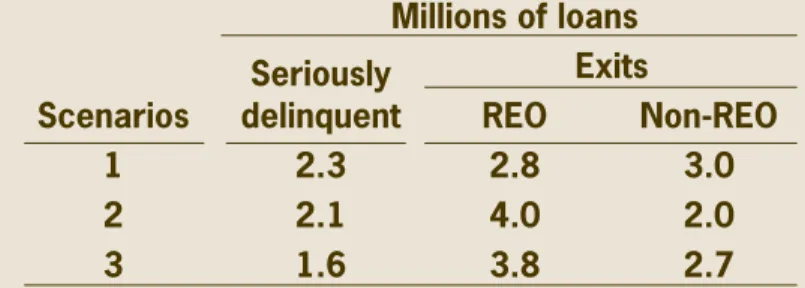
Table 1. Projected Numbers of Loans in
Different Stages, June 2013
0 100 200 300 400 500 600 700 800 900 6/10 12/10 6/11 12/11 6/12 12/12 6/13 Thousands Scenario 1 Peak—555,693 (10/2010) Scenario 2 Peak—719,757 (7/2011) Scenario 3 Peak—825,559 (12/2010)
Source: Author’s calculations. Source: Author’s calculations.
Millions of loans Seriously
delinquent
Exits
Scenarios REO Non-REO
1 2.3 2.8 3.0
2 2.1 4.0 2.0
is worth considering. The assumption is that these fl ows will fall over the three-year projection period from current levels to what was typical prior to the recession. How-ever, given current forecasts for various macroeconomic variables, it seems optimistic to think that households will experience the same relatively low levels of fi nancial distress in 2013 that they experienced prior to 2007. This suggests that even fairly optimistic expectations imply elevated REO levels for a few years to come. Importantly, these elevated REO levels arise and persist despite possible changes to pre-REO processes, as shown by the second two simulations.
Aside from differences in REO levels, each scenario also produces different predictions about how loans will work through the system and what routes they may take to exit. Table 1 shows the numbers of loans in each simulation that have transitioned to various states by the end of the projec-tion period. In scenarios 2 and 3, roughly 4.0 million loans will have transitioned to REO during the three-year period. This is at least a million more than we observe in scenario 1. Essentially, the changes to transition rates in scenarios 2 and 3 increase the throughput of loans, so that more loans move through to REO. The fl ip-side of this is that more loans remain in serious delinquency in scenario 1.
But the gap in the ending stock of seriously delinquent loans between scenarios 2 and 1 is fairly small. That’s because far fewer loans make a non-REO related exit from the system in scenario 2. The highest likelihood of making a non-REO exit (i.e., transitioning to a less serious state of delinquency, becoming current, or paying off) occurs when a loan is in the 90+ day delinquency pool. Because we signifi cantly increase the transition rate from 90+ day delinquency to foreclosure in scenario 2, we more quickly draw down the size of this pool. As a consequence, we ef-fectively deprive more loans of the opportunity to exit the system through some means other than REO.
Conclusion
These simulations estimate the timing and number of REO properties that might ultimately emerge from the substantial stock of homes currently in the so-called shadow inventory. Will this stock—which has been able to accumulate partially as a consequence of various attempts to help homeowners avoid losing their homes—ultimately fl ood the market, and put even more downward pres-sure on prices? Such a development would be worrisome, since falling prices would push more homeowners “under water,” which could in turn induce more borrowers to default.
The admittedly simple scenarios outlined above suggest that if loans were to move through 90+ day delinquency and foreclosure at rates common prior to the onset of the crisis, we would indeed see a more substantial stock of REO properties enter the market. To this extent, scenario 1 looks like a preferable outcome, in that the outstand-ing stock of REO properties rises only modestly, before beginning to diminish. This path seems likely to have less pronounced price effects than the larger increases in REO properties associated with scenarios 2 and 3. However, one important element not captured by these simulations is the quality of the properties that emerge as REOs.
The slower rate of REO production in scenario 1 is also associated with longer foreclosure and delinquency dura-tions. The problem with this circumstance is that as a borrower falls further and further behind on his payments, it becomes increasingly unlikely that he will ever be able to repay arrearages and reinstate his mortgage. At this point, if he continues to occupy his home, he may be disinclined to maintain it as an owner would. Alternatively, a borrow-er may decide to leave his propborrow-erty during the course of a foreclosure. In this instance, the home may sit vacant for months until the foreclosure is fi nalized, a potential target for thieves and vandals. These instances illustrate that longer timelines for foreclosure and delinquency are likely to reduce property values, and not only for the foreclosed properties, but also for those in the neighborhood. As a consequence, just like a large increase in REO properties, this too could induce additional foreclosures.
Determining which of the above scenarios, or any potential REO path, is likely to have the most benign consequences for prices, and accordingly for foreclosures, requires under-standing which of these two effects is more dominant.
Guhan Venkatu is an economist at the Federal Reserve Bank of Cleveland. The views he expresses here are his and not necessarily those of the Federal Reserve Bank of Cleveland or the Federal Reserve Board.
Economic Commentary is published by the Research Department of the Federal Reserve Bank of Cleveland. To receive copies or be placed on the mailing list, e-mail your request to [email protected] or fax it to 216.579.3050. Economic Commentary is also available on the Cleveland Fed’s Web site at www.clevelandfed.org/research.
PRSRT STD U.S. Postage Paid
Cleveland, OH Permit No. 385 Federal Reserve Bank of Cleveland
Research Department P.O. Box 6387 Cleveland, OH 44101
Return Service Requested:
Please send corrected mailing label to the above address.
Material may be reprinted if the source is credited. Please send copies of reprinted material to the editor at the address above.