Robust estimation of the vector autoregressive model by a trimmed least squares procedure.

ROBUST ESTIMATION OF THE VECTOR AUTOREGRESSIVE MODEL BY A TRIMMED LEAST SQUARES PROCEDURE

KRISTEL ]OOSSENS • CHRISTOPHE CROUX

Robust estimation of the vector autoregressive model

by a trimmed least squares procedure

Kristel

J

oossens*

and

Christophe Croux*

K. U. Leuven

Abstract

The vector autoregressive model is very popular for modeling multiple time series. Estimation of its parameters is done by a least squares procedure. However, this estimation method is unreliable when outliers are present in the data, and there is a need for robust alternatives. In this paper we propose to estimate the vector autoregressive model by using a trimmed least squares estimator. We show how the order of the autoregressive model can be determined in a robust way, and how confidence bounds around the robustly estimated impulse response functions can be constructed. The resistance of the estimators to outliers is studied on real and simulated data.

1

Introduction

The use of autoregressive models for predicting and modeling univariate time senes IS

standard and well known. In many applications, one does not observe a single time series, but several series, possibly interacting which each other. For these multiple time series the vector autoregressive model has become very popular, and is described in standard textbooks on time series (e.g. Brockwell and Davis 2003, Chapter 7; Stock and Watson *Department of Applied Economics, Katholieke Universiteit Leuven, Naamsestraat 69, B-3000 Leuven, Belgium, E-mail: {kristel.joossens.christophe.croux}@econ.kuleuven.be.

2003, Chapter 14). In this paper we propose a robust procedure to estimate vector autoregressive models, to select their order, and to construct confidence bounds around the impulse response functions.

Let {Yt I

t

E Z} be a p-dimensional stationary time series. The vector autoregressive model of order k, denoted by VAR(k), is given by

Yt

=

B~

+

B~Yt-1

+ ... +

B~Yt-k

+

Ct, (1.1 )

with Yt a p-dimensional vector, the intercept parameter B~ a vector in IRP and the slope parameters B1 , . . . ,Bk being matrices in IRPxP. Throughout the paper M' will stand for

the transpose of the matrix M. The p-dimensional error terms Ct are supposed to be

independently and identically distributed with center zero and scatter matrix~. The latter means that the density of Ct is of the form

(1.2)

with ~ a positive definite matrix, called the scatter matrix and 9 a positive function. If the second moment of Ct exists, then ~ will be (proportional to) the covariance matrix

of the error terms. Existence of a second moment, however, will not be required for the robust estimator. We focus on the unrestricted VAR( k) model, where no restrictions are put on the parameters Bo, B1 , . . . ,Bk .

Suppose that the multivariate time series Yt is observed for

t =

1, ... ,T. The vector autoregressive model (1.1) can be rewritten as a multivariate regression model

(1.3)

for

t =

k

+

1, ... , T and with Xt

=

(1, Y~-l" .. , Y~-k)' E IRq, where q

=

pk

+

1. The matrix

B =

(Bb,

B~, ... ,B~)' E IRqxp contains all unknown regression coefficients. In the language

of regression, X

=

(Xk+1' ... ,XT)' E IRnxq is the design matrix and Y

=

(Yk+1, ... ,YT)' E

the regression parameter B in (1.3) is given by the well known formula

while the scatter matrix I: is unbiasedly estimated by

A 1 A A

I:oLs = - - ( Y - XBoLs)'(Y - XBoLs ).

n-p

(1.4)

In applied time series research, one is aware of the fact that outliers can seriously affect parameter estimates, model specification and forecasts based on the selected model. For example, in business and economic data, it is common to see unusually low observations followed by unusually high observations or vice versa. Outliers in time series can be of different natures (Fox 1972), the most well known types being additive outliers and innovational outliers. If we consider the autoregressive model (1.1), then we say that Yt is an additive outlier if only its own value has been affected by contamination. On the other hand, we have an innovational outlier if the error term Ct in (1.1) is contaminated.

Innovational outliers will therefore has an effect on the next observations as well, due to the dynamic structure in the series. Additive outliers only have an isolated effect.

Several procedures to detect different types of outliers for univariate time series have been proposed (e.g. Chang, Tiao and Chen 1988, Gerlach, Carter and Kohn 1999 and Wu, Ravishanker and Hosking 1993). Bianco, Garcia Ben, Martinez and Yohai (2001) and Riani (2004) propose diagnostic procedures based on robust estimators. Other robust estimators for univariate ARMA models have been proposed by Bustos and Yohai (1986) and De Luna and Genton (2001). All of the above studies focus on a single series.

The aim of this paper is to propose a robust estimation procedure for the multivariate autoregressive model, the most popular models for multiple time series analysis. Previous work on robust multivariate time series analysis uses estimators of the generalized M-type, which are known to have a low robustness in higher dimensions. Franses, Kloek and Lucas (1999) used generalized M-estimators and apply them on weekly scanning data. Garda Ben, Villar and Yohai (1999) use so-called residual autocovariance estimators, being an affine equivariant version of the estimators of Li and Hui (1989). Also the estimators of

Garcia Ben et al (1999) are solutions of estimating equations. The latter may well have multiple solutions, which may not all correspond to robust solutions.

A common practice for handling outliers in a multivariate process is to first apply univariate techniques to the component series in order to remove the outlier, followed by treating the adjusted series as outlier-free and model them jointly. But this procedure encounters several difficulties. First, in a multivariate process, contamination in one component may be caused by an outlier in the other components. Secondly, a multivariate outlier cannot always be detected by looking at the component series separately, since it can be an outlier for the correlation structure only. Therefore it is better to cope with outliers in a multivariate framework. Tsay, Perra and Pankratz (2000) discuss the problem of multivariate outliers in detail.

To obtain a resistant estimator for the vector autoregressive model, we will replace the classical multivariate least squares estimator in (1.3) by a highly robust estimator. We will use the Multivariate Least Trimmed Squares estimator, introduced by Agull6, Croux and Van Aelst (2002). This estimator is defined by minimizing a trimmed sum of a squared Mahalanobis distances, and can be computed by a fast algorithm. The procedure also provides a natural estimator of the scatter of the residuals, which can then be used for model selection criteria. We present this estimator in Section 2. Section 3 explains how to determine in a robust way the autoregressive order of the model. In Section 4 confidence bounds around the impulse response functions obtained from the robust estimates are constructed. The robustness of the estimates is studied by means of several simulation experiments in Section 5, showing the effect of outliers on the estimation of the model and on the impulse response functions. In Section 6, the robust VAR methodology is applied on a real data set. Finally, Section 7 contains some conclusions.

2

The multivariate least trimmed squares estimator

The unknown parameters of the VAR( k) will be estimated via the multivariate regression model (1.3). For this the Multivariate Least Trimmed Squares estimator (MLTS), based on the idea of the Minimum Covariance Determinant estimator (Rousseeuw and Van

Driessen 1999), will be used. The MLTS selects the subset of h observations having the

property that the determinant of the covariance matrix of its residuals from a least squares fit, solely based on this subset, is minimal.

Consider the data set Z

=

{(Xt, Yt), t

=

k

+

1, ... , T}

c

lRp_{+q , and for any B E lR}pxq

denote rt(B)

=

Yt - B'Xt the corresponding residuals. Let 7-i

=

{H C {k

+

1, ... , T} I

#H = h} be the collection of all subsets of size h. For any subset H E 7-i, let BOLS (H) be the classical least squares fit based on the observations of the subset

where XH and YH are submatrices of X and Y, consisting of the rows of X, respectively

Y, having an index in H. The corresponding scatter matrix estimator computed from this subset is then

The MLTS estimator is now defined as

BMLTS(Z)

=

BOLS(iI) where iI

=

argmin det I:oLs(H), HEH

and the associated estimator of the scatter matrix of the error terms is given by

I:MLTS

(H)

= I:OLS (iI).

(2.1 )

(2.2)

Equivalent characterizations of the MLTS estimator were given by Agull6, Croux and Van Aelst (2002). They proved that any

B

E lRpxq _{minimizing the sum of the h smallest}

squared Mahalanobis distances of its residuals (subject to det 2:

=

1) is a solution of (2.1). In mathematical terms,

h

BMLTS

=

argmin

L

d;:n(B, 2:).

Here d1:n(B,

2::) ::; ... ::;

dn:n(B,

2::)

is the ordered sequence of the Mahalanobis distances

d;(B,

2::) =

rs(B)'2::- 1rs(B). Therefore, we see that the MLTS-estimator minimizes the sum of the h smallest squared distances of its residuals, and is therefore the multivariate

extension of the Least Trimmed Squares (LTS) estimator of Rousseeuw (1984).

Since the efficiency of the MLTS estimator is rather low, we will use the reweighted version to improve the performance of the MLTS. If B MLTS and

I:

MLTS denote the

ini-tial MLTS estimates, then the one-step Reweighted Multivariate Least Trimmed Squares (RMLTS) estimates are defined as

(2.3)

where J

=

{j

I

d;

(BMLTS,

t

MLTS ) ::; qo} and qo

=

X~,l-O is the upper 6"-quantile ofax2

distribution with q degrees of freedom. Here 6" is the trimming fraction in the reweighting step and Co is a consistency factor to obtain consistent estimation of I; at the model distribution (1.2) of the error terms. In the case of multivariate normal error terms it has been shown (e.g. Croux and Haesbroeck 1999) that Co

=

(1- 6")/FX2 (qo). Here

p+2

Fx~ is the cumulative distribution function ofax2 _{distribution with q degrees of freedom.}

The idea is that outliers have large residuals with respect to the initial robust MLTS estimator, resulting in a large residual Mahalanobis distance

d;

(BMLTS,

I:

MLTS ). If this

Mahalanobis distance is above the critical value X~,l-O' then the observation is flagged as an outlier. The final RMLTS is based on the observations not detected as outliers. In this paper, we set 6"

=

0.01 and take as trimming portion for the initial MLTS estimator

1 - h/n ~ 25%

=

CY.

3

Determining the Autoregressive Order

To select the order of the vector autoregressive model, criteria for different orders are computed and an estimator of the optimal order is obtain by minimizing this criterion. Most of these criteria are in terms of the value of the log likelihood lk of the VAR( k).

U sing the model hypothesis on the error terms, we get

T

lk =

L

g(E~~-lEt)

-

¥

log

det~.

t=k+l

Recall that n

=

T - k. When error terms are multivariate normal the above leads to

(3.1 )

The log likelihood will depend on the autoregressive order via the estimate of the covari-ance matrix of the residuals. For the ordinary least squares estimator we have

1 T

~OLS

= - - """'

Et(k)E~(k),

n-p D

t=k+l

where the Et(k) are the residuals corresponding with the estimated vector autoregressive model of order k. Using the trace properties, we have that the last term in (3.1) equals the constant -(n-p)p/2 for the OLS estimator. To prevent that outliers might affect the estimation of the VAR models and therefore also the estimation of the criteria, we will estimate ~ by the robust reweighted multivariate least trimmed squares estimator instead of the ordinary least squares estimator. When using the RMLTS, discussed in Section 2, we get

with J as in (2.3) and m the number of elements in J. Now, the last term in (3.1) becomes

-(m - p)p/2co, where the value of m might depend on the selected order k.

We will consider the following three criteria: the popular Akaike info criterion (Akaike 1973) defined as

-2 2

AIC(k)

=

- l k

+

-(kp

+

l)p,

n n

the Hannan-Quinn criterion (Hannan & Quinn 1979) given by

Q(k) -2l 2log(log(n)) (k )

H

= -

k

+

p+ 1 p,

and the Schwarz criterion (Schwarz 1978) which equals

SC(k)

=

-2_Zk + log(n)(kp+l)p.

n n

In all three criteria, (kp

+

l)p 1S the number of unknown regresslOn parameters and

penalizes for model complexity.

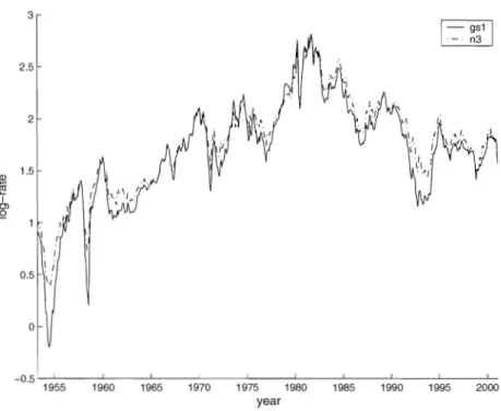
To illustrate that outliers affect the lag length criteria, we use the bivariate time series "gsln3" (Tsay 2002, p. 324~325). The first series "gsl" is the I-year Treasury constant maturity rate, and the second series "n3" is the 3-year Treasury constant maturity rate. The data are monthly and obtained from the Federal Reserve Bank of St Louis. The sampling period is from April 1953 to January 2001. As in the book of Tsay (2002), we work with the log-transformed versions of both series. From the plot of the two log transformed series (Figure 1), it can be seen that there might be some outliers around the years 1954 and 1958.

In Table 1 the lag length criteria using the ordinary least squares estimator and the reweighted multivariate trimmed least squares estimator are represented. The information criteria clearly depend on the chosen estimator. For example, when using the AIC the classical method suggests a VAR(8) model while the robust indicates a VAR(6) model. On the other hand the Schwarz criterion selects an optimal order 3 for both estimators. Since the latter criterion yields a consistent estimate of the optimal order (Hannan 1980) we continue the analysis with k

=

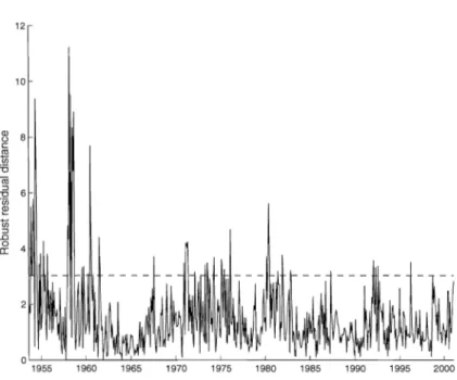
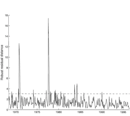
3.

After estimating the VAR(3) model with the robust RMLTS estimator, the corre-sponding robust residual distances dt (BRMLTS, tRMLTS) are computed. Figure 2 displays

these distances with respect to the time index, and indicates outlying observations. Since residual squared distances follow a X~ distribution, it is common to compare these dis-tances with the critical value Xp,O.99 (Rousseeuw and Van Zomeren 1991). Figure 2 reveals that several suspectable high residuals are detected, indicating presence of huge outliers around the years 1954 and 1958. Therefore it seems appropriate to make use of robust methods for further analysis of this data set.

3 2.5 2 1.5 OJ ~ I OJ .2 r \ I \ i 0.5 \j o -0.5 '--'-_ _ . L - . _ - - ' - - _ - - ' - - _ - - - ' _ _ - ' - - - - _ . - L - _ - - ' -_ _ ' _ ' -1955 1960 1965 1970 1975 1980 1985 1990 1995 2000 year

Figure 1: Time plot ofthe log U.S. monthly interest rates from April 1953 to January 200l. The solid line represents the I-Year Treasury constant maturity rate and the dot-dashed line represents the 3-Year Treasury constant maturity rate.

Table 1: Lag length criteria using the OLS and RMLTS estimator for the "gsln3" series.

k 1 2 3 4 5 6 7 8

Based on

OLS

estimation

AlC

-7.3552 -7.5823 -7.6179 -7.6261 -7.6149 -7.6078 -7.6268 -7.6276 HQ -7.3374 -7.5526 -7.5763 -7.5726 -7.5494 -7.5302 -7.5372 -7.5258

SC

-7.3096 -7.5062 -7.5113 -7.4889 -7.4470 -7.4090 -7.3972 -7.3669 Based on

RMLTS

estimation

AlC

-7.4386 -7.6282 -7.6795 -7.6997 -7.6943 -7.7490 -7.6961 -7.7118 HQ -7.4208 -7.5985 -7.6380 -7.6461 -7.6288 -7.6714 -7.6065 -7.6101

SC

-7.3930 -7.5522 -7.5730 -7.5624 -7.5264 -7.5502 -7.4665 -7.4512

12

10

1960 1965 1970 1975 1980 1985 1990 1995 2000

Figure 2: Robust residual distances for the "gsln3" series based on the robust RMLTS estimator of a VAR(3) model. The dashed line represents the critical value X2,O.99 =

3.0349.

4

Impulse response function

After selecting and estimating the VAR model, it is common and instructive to look at the Impulse response Function (IRF), which permits to quantify variable responses to shocks on different horizon lengths (Hamilton 1994, chapter 11). The impulse response functions are defined as follows. Let B(L) be the autoregressive polynomial Ip - B~L ... - B~Lk.

We can write the vector autoregressive model as B(L)Yt = Bb

+

Ct, or Yt = B(L)-IBb

+

B(L)-ICt, which can rewritten as an infinite moving average model

Yt

=

a

+

Ct

+

A1Ct-1

+ ... +

Azct-z

+ ...

where

a

is a vector and

AI,

A

2 , . . . ,

A

z, ...

are p

x

p matrices, depending on the

pa-rameters in B. The function mapping l on (AZ)ij, for l = 1,2,3, ... is called an impulse response function. It measures the response of component i of Yt to an impulse of one unit in component j of Ct-Z. Letting the indices i and j range between 1 and p, results in p2 impulse response functions. In practice B is estimated, yielding an estimated IRF. Using

a robust estimate of

B,

yields then a robustly estimated IRF. In the sequel, we consider two methods to construct confidence bounds around these estimated IRFs.

To construct the analytic confidence bounds, we start from the asymptotic normality of the estimators in the multivariate regression model (1.3):

~ f t 1

vT(vecB -

vecB) ---+ Np(pk+l) (0, cp~ ® Q- ). (4.1 )

Here Q = E[XtX~], with Xt as in Section 1, and "vec" is the operator which vectorizes a

matrix and ® stands for the kronecker product. The constant cp depends on the chosen

estimator. For the OLS estimator we have cp

=

1, and for the RMLTS the value of cp

will be larger than 1 and can be retrieved from the asymptotic variance of the RMLTS estimator for the multivariate regression model (Agullo, Croux and Van Aelst 2002). Note that cp not only depends on the dimension, but also depends on the trimming fraction

ex of the initial MLTS estimator and on the trimming fraction b used in the reweighting step. For the RMLTS we have

with C = 1 - Fo/(l - b) where Fo = Fx2 _p+2 (Xp2 _, 1-0) and Fa = Fx2 _p+2 (Xp2_, 1_a)'

By using the Delta method, as in Hamilton (1994, page. 186), we get from (4.1) that

where

Gz

=

ovecAz(B)

o(vecB)! .

Standard errors around the values (AZ)ij of the IRFs are then obtained as the square roots of the diagonal elements of cp~Oz(t ®

(>-1)0;.

Here we take

t

as in (2.3), and

(>

= average XtX~ with J the set of indices used in the definition of the RMLTS estimator.

tEJ

that Gz can be calculated recursively via the formula

z

Gz

=

L

[A8 - 1 ® (Onl AZ- 8 AZ- 8 - 1 ••• AZ- 8 - k - 1)] ,

8=1

where Onm is a zero matrix of size

n

x m. The matrices

Az

in the above expressions need then to be estimated by

Az

(B).

We can also obtain Monte Carlo confidence bounds using a parametric bootstrap procedure. We first estimate the model from the original data. Then we generate 1000 series according to the estimated VAR( k) model, with errors following a multivariate normal distribution with mean zero and covariance matrix~. From these 1000 generated series, 1000 impulse response values can be computed. By sorting these values and taking the 2.5% and 97.5% quantile, 95% confidence bounds can be constructed for the impulse response functions.

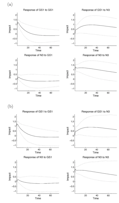
The analytic and Monte Carlo confidence intervals around the IRFs estimated by the robust procedure have been computed for the "gsln3" -data containing the Maturity rates GS1 and N3 (see Figure 3) for the robust RMLTS estimator. We see that the impulse response functions for the analytic method and the Monte Carlo method are very similar. The Monte Carlo based 95% confidence bounds are marginally larger and are less smooth in comparison with the analytic confidence bounds.

It is seen from Figure 3 that the effect of a unit shock at the innovation of GS1 on the response of GS1 is significant up to 11 months. On the other hand the variable N3 is non-responsive to such a shock. The effects of a unit shock in the innovation series driving N3 are more important: the response of GS1 is significant to almost 3 years and the response of N3 is significant up to almost 4 years.

5

Robustness of the estimator

In order to look at the robustness of the estimates, we will perform a simulation study comparing the OLS estimator with the robust RMLTS estimator. Consider a bivariate

( a) 2 1.5 "0 1 . ell 0.5 0. E 0 -0.5 -1 2 1.5 "0 ell 0.5. 0. E 0 -0.5 -1 (b) "0 ell 0. E "0 2 1.5 .' 1 0.5 0 -0.5 -1 2 1.5 Response of GS1 to GS1 20 40 60 Time Response of N3 to GS1 20 40 60 Time Response of GS1 to GS1 20 40 Time 60 Response of N3 to GS1 ~ 0.5 .' ... . E o -0.5 -1 20 40 Time 60 2 1.5 "0 ell _{0.5 :'} 0. E 0 -0.5 -1 Response of GS1 to N3 20 40 Time 60 Response of N3 to N3 2 1 . 5 · · · . "0 1 '. ~ 0.5 E "0 ell 0. E "0 o -0.5 -1 2 1.5 0.5 :' 0 -0.5 -1 2 1.5' .' 1 '. ~ 0.5 E o -0.5 -1 20 40 Time 60 Response of GS1 to N3 20 40 Time 60 Response of N3 to N3 20 40 Time 60

Figure 3: The impulse response functions (solid lines) for the "gsln3" data based on VAR(3) models estimated by the robust RMLTS estimator, together with its (a) analytic; (b) Monte Carlo confidence bounds (dotted lines).

time series generated according the VAR(2) model

(Y1,t)

(.10)

+

(.40 .03)

(Y1,t-1)

+

(.100

Y2,t

.02 .04 .20

Y2,t-1

.010 .005) .080

(Y1,t-2)

+

(E1,t)

Y2,t-2

E2,t

(5.1) where

Et

r v N2(0,~) with

~

=

(1 .2).

.2 1 (5.2)

The aim is to look at the effect of the outliers on the parameter estimates. Since there are 10 parameters to be estimated for each equation, we look at the total bias and total Mean Squared Error (MSE) as performance measures. The bias is computed as

Bias = ( . ) 2 q p 1 nS1m A

LL -.

L

B f j - B i j , nS1m i=l j=l s=l

where BS, for s = 1, ... , nsim, is the estimate obtained from the s-th generated series, B is the true parameter value and nsim= 1000 the number of simulations. The MSE equals

MSE = """ """ - . """ (BS _{- Bi}

.)2

q p [ 1 nSlm

1

D D nS1m D 2J J

i=l j=l s=l

The classical and robust estimators are used to estimate the VAR(2) model for the un-contaminated series and the un-contaminated series, where outliers are added.

5.1

Additive outliers

After generating the series of length T =500, additive outliers are introduced. The

con-tamination is done by randomly selecting m bivariate observations, and adding the value 10 to all the components of the selected observations. We have considered different con-tamination levels, ranging from one single up to 40 additive outliers.

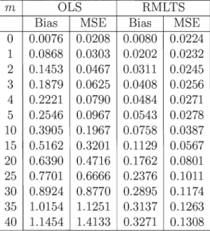
Table 2: Simulated Bias and Mean Squared error for the classical (OLS) and robust (RMLTS) estimator of a bivariate VAR(2) model, in presence of m additive outliers in a series of length 500.

m OLS RMLTS

Bias MSE Bias MSE

0 0.0076 0.0208 0.0080 0.0224 1 0.0868 0.0303 0.0202 0.0232 2 0.1453 0.0467 0.0311 0.0245 3 0.1879 0.0625 0.0408 0.0256 4 0.2221 0.0790 0.0484 0.0271 5 0.2546 0.0967 0.0543 0.0278 10 0.3905 0.1967 0.0758 0.0387 15 0.5162 0.3201 0.1129 0.0567 20 0.6390 0.4716 0.1762 0.0801 25 0.7701 0.6666 0.2376 0.1011 30 0.8924 0.8770 0.2895 0.1174 35 1.0154 1.1251 0.3137 0.1263 40 1.1454 1.4133 0.3271 0.1308

the Bias and MSE grows for an increasing number of outliers. The increase in Bias and MSE is much faster for the method using OLS. Using the robust estimator instead of OLS leads to a small loss in efficiency at the model when no outliers are present. When only even one outlier is introduced, the RMLTS is already more efficient, and the gain in MSE for the RMLS becomes highly substantial for the larger amounts of outliers. associated impulse response functions.

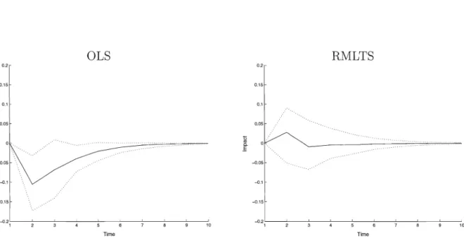
The robustness of the estimates of the impulse response function is studied as well. For each of the nsim=1000 simulated series, the IRF is computed. A plot of the averaged impulse response functions, together with the 5% and 95% quantiles over all the generated IRFs is made in Figure 4. This figure represents the impulse response functions of the response of Variable 1 to a unit shock in the innovation term of Variable 2, once as estimated by using ordinary least squares estimators, and once by using the reweighted multivariate least trimmed squares estimators. We hardly see any difference between the

but the quantiles are somehow wider while using the robust estimator, since the RMLT8 is a bit less efficient when no outliers are present. We now add 5 additive outliers in order to look at their effect on the impulse response functions. From Figure 5 we see that the average IRFs using the robust estimator looks more like the average IRFs of the uncontaminated data in Figure 4. But, when using the classical estimator, there is a change of the shape in the impulse response function. Hence, and without much surprise, the non-robustness of the OL8 estimator is also reflected in the

5.2

Innovational outliers

Instead of contaminating the series with additive outliers, we look now at the effect of innovational outliers. To generate these innovational outliers, we randomly select a num-ber m of innovation terms in (5.1) and add 10 to the first component of the innovations, to come to the contaminated innovations series

Ef.

These are then used to generate the bivariate series according to (5.1), but with Et replaced by

Ef.

Recall that innovational

outliers have a more persistent effect on the series Yt then additive outliers. The Bias and M8E when estimating the uncontaminated (m

=

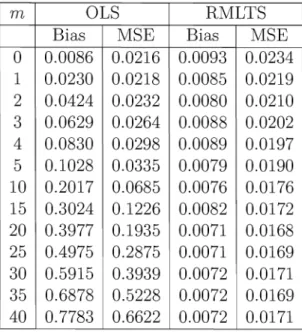
0) and contaminated series are given in Table 3, for as well the classical as the robust estimation.

The Bias and M8E for OL8 grow quite fast for an increasing number of innovational outliers, although at a smaller rate as for contamination with additive outliers. For the robust estimator we see a small decrease of the Bias and M8E, implying that the robust procedure becomes more efficient in presence of innovational outliers. This is due to the fact that an innovational outlier in the time series result in a single vertical outlier, but also in several good leverage points when estimating the autoregressive model. The robust method can cope with the vertical outlier and takes profit of the good leverage points to decrease the M8E. The OL8 estimator gets biased due to the vertical outliers, but the presence of the good leverage points explains why the effect of innovational outliers is less strong as for additive outliers. Note that when no outliers are present, the RMLT8 is again very close to OL8, the loss in efficiency being marginal.

OLS RMLTS 0.2 0.2 0.15 0.15 0.1 0.1 0.05 0.05 0 R :l. E E -0,05 -0.05 -01 -0.1 -0.15 -0.15 -0.2 -0.2 1 10 1 10 Time Time

Figure 4: Simulated average impulse response functions (solid lines) and the 5% and 95% quantiles (dotted lines) for a bivariate VAR( 2) model using the 0 LS estimator (left) and the RMLTS estimator (right).

OLS RMLTS 0.2 0.2 0.15 0.15 0.1 0.1 0.05 0.05 R E -0,05 -0.1 -0.15 -0.15 -0.2 10 1 10 -0.2 ,'----'---:---~-':---~_____::__~-____o_-___c Time Time

Table 3: Bias and Mean Squared error for the classical (OLS) and robust (RMLTS) estimator of a bivariate VAR(2) model, in presence of m innovational outliers in a series of length 500.

m OL8 RMLT8

Bias M8E Bias M8E

0 0.0086 0.0216 0.0093 0.0234 1 0.0230 0.0218 0.0085 0.0219 2 0.0424 0.0232 0.0080 0.0210 3 0.0629 0.0264 0.0088 0.0202 4 0.0830 0.0298 0.0089 0.0197 5 0.1028 0.0335 0.0079 0.0190 10 0.2017 0.0685 0.0076 0.0176 15 0.3024 0.1226 0.0082 0.0172 20 0.3977 0.1935 0.0071 0.0168 25 0.4975 0.2875 0.0071 0.0169 30 0.5915 0.3939 0.0072 0.0171 35 0.6878 0.5228 0.0072 0.0169 40 0.7783 0.6622 0.0072 0.0171

6

Example

We illustrate the use of the robust estimation of the parameters of a vector autoregressive model on a real time series, called "housing" data (Diebold 2001, p. 109). Housing is a bivariate series of monthly data of housing starts and housing completions from January 1968 up to June 1996. To find the optimal order of the vector autoregressive model, the ro bust lag length criteria are used and each of them suggests a VAR( 4) model. After estimating the model, robust residuals distances are computed and plotted in Figure 6. Two severe outliers are detected, together with two other extreme observations. Due to the presence of these atypical observations, it is indeed advisable to use a robust estimation procedure.

Impulse response functions resulting from the estimated VAR( 4) model using OL8 and RMLT8 are presented in Figure 7. In all four IRF we see that the effect of a shock is underestimated when the OL8 estimator is used with respect to using the RMLT8 estimator. The robust IRFs are also somewhat smoother. A unit shock in the innovation

for the variable "housing starts" gives rise to a large response on the completions series (and also on its housing starts series). On the other hand, a unit shock in the innovations of the completions series has only a limited impact on both series. Since outliers are present in the data, we think that more confidence should be given to the robust analysis.

7

Conclusion

For multivariate time series it may occur that correlation outliers can be present, which are not necessarily visible in plots of the single univariate series. Development of robust procedures for multiple time series analysis is therefore even more important than for univariate time series analysis.

In this paper we show how robust multivariate regression estimators can be used to estimate Vector Autoregressive models. Focus was on the reweighted multivariate least squares estimators, since the objective function defining this estimator is closely related to several information criteria. Of course, other robust multivariate regression estimators can be used as well (e.g. the MM estimators of Tatsuoka and Tyler 2000 or the robust covariance based estimators of Rousseeuw et al 2004). Software to robustly estimate the VAR model is available at http://www.econ.kuleuven.be/kristel.joossens. and was used to analyze the real data set of Section 6. This software provides robust distances as a tool for outlier detection, computes different robust lag-length criteria, as well as robustly estimated impulse response functions. These impulse response functions are used in applied multivariate time series especially in economics for interpreting the estimated VAR model. We also provide the confidence bounds around this robust impulse response functions ..

The simulation experiments in Section 5 clearly illustrated the advantage of using the reweighted multivariate least trimmed squares estimator instead of the classical approach. If there are no outliers in the data set present, the robust estimator performs almost as good as the classical estimator. But it there are outliers, then bias and MSE remain under control when using the robust estimator.

18 16 14 ~ 12 c CO t5 ~ 10 CO :::J TI ·00 ~ t5 :::J ..0 fE 6 4

Figure 6: Robust residual distances for the housing data set. The dashed line represents the critical value.

Response of starts to starts

0.8 \ / _.... 0.6 " "0

"

co 0.4 0-E 0.2 " _" 0 -0.2 20 40 60 Time

Response of completions to starts

0.8 0.6 "0 - , co 0.4 / .... 0- J .... E I _" 0.2 I " " 0 -0.2 20 40 60 Time 0.8 0.6 "0 co 0.4 0-E 0.2 0.8 0.6 "0 CO 0.4 0-E 0.2 ' 0 -0.2

Response of starts to completions

20 40

Time

60

Response of completions to completions

"

"

20 40 60

Time

Figure 7: The impulse response functions for the housing data set, based on a VAR(4) model estimated by the classical OL8 estimator (solid line) and the robust RMLT8 esti-mator. The variables in the housing data set are starts and completions.

research has been supported by the Research Fund K.U. Leuven and the "Fonds voor Wetenschappelijk Onderzoek" (Contract number G.0385.03).

References

Agull6, J., Croux, C., and Van Aelst, S. (2002), "The multivariate least trimmed squares estimator," Research report, Dept. of Applied Economics, K.U.Leuven, Belgium. Akaike, H. (1973), "Information theory and an extension of the maximum likelihood

principle," in 2nd International Symposium on Information Theory, eds. Petrov, B. N. and Csaki, F., Academiai Kiad6: Budapest, pp. 267~281.

Bianco, A. M., Garcia Ben, M., Martinez, E. J., and Yohai, V. J. (2001), "Outlier de-tection in regression models with ARIMA errors using robust estimates," Journal of

Forecasting, Vol. 20, 565~579.

Brockwell, P. J. and Davis, R. A. (2003), Introduction to Time Series and Forecasting, Wiley: New York, 2nd ed.

Bustos, H. and Yohai, V. J. (1986), "Robust estimates of ARMA models," Journal of the

American Statistical Association, Vol. 81(393), 155~ 159.

Chang, 1., Tiao, G. C., and Chen, C. (1988), "Estimation of time series parameters in the presence of outliers," Technometrics, Vol. 30, 193~204.

Croux, C. and Haesbroeck, G. (1999), "Influence function and efficiency of the MCD-scatter matrix estimator," Journal of Multivariate Analysis, Vol. 71, 161~190.

De Luna, X. and Genton, M. G. (1967), "Robust simulation-based estimation of ARMA models," Journal of Computational and Graphical Statistics, Vol. 10(2), 370~387. Diebold, F. X. (2001), Elements of Forecasting, South Western College Publishing, 2nd

Fox, A. (1972), "Outliers in time series," Journal of the Royal Statistical Society, Series

B, Vol. 34(3), 350-363.

Franses, H., Kloek, T., and Lucas, A. (1999), "Outlier robust analysis of long-run mar-keting effects for weekly scanning data," Journal of Econometrics, Vol. 89, 293-315.

Garda Ben, M., Martinez, E. J., and Yohai, V. J. (1999), "Robust estimation in vector autoregressive moving average models," Journal of Time Series Analysis, Vol. 20(4),

381-399.

Gerlach, R., Carter, C., and Kohn, R. (1999), "Diagnostics for time senes analysis,"

Journal of Time Series Analysis, Vol. 20(3), 309-330.

Hamilton, J. D. (1994), Time Series Analysis, Princeton University Press.

Hannan, E. J. (1980), "The estimation of the order of an ARMA process," Annals of Statistics, Vol. 8, 1071-1081.

Hannan, E. J. and Quinn, B. G. (1979), "The determination of the order of an autore-gression," Journal of the Royal Statistical Society, Series B, Vol. 41(2), 190-195.

Li, W. K. and Hui, Y. V. (1989), "Robust multiple Time series modelling," Biometrika,

Vol. 76(2), 309-315.

Riani, M. (2004), "Extensions of the forward search to time series," Studies in Non Linear Dynamics and Econometrics, Vol. 8(2), Article 2.

Rousseeuw, P. J. (1984), "Least median of squares regression," Journal of the American Statistical Association, Vol. 79, 871-880.

Rousseeuw, P. J. and Van Driessen, K. (1999), "A fast algorithm for the minimum co-variance determinant estimator," Technometrics, Vol. 41, 212-223.

Rousseeuw, P. J., Van Driessen, K., Van Aelst, S., and Agullo, J. (2004), "Robust multi-variate regression," Technometrics, Vol. 46(3), 293-305.

Rousseeuw, P. J. and Van Zomeren, B. C. (1991), "Robust distances: simulations and cutoff values," in Directions in Robust Statistics and Diagnostics, part II, eds. Stahel,

W. and Weisberg, S., Springer Verlag: New York, vol. 34 of the IMA Volumes in Mathematics and Its Applications, pp. 195-203.

Schwarz, G. (1978), "Estimating the dimension of a model," Annals of Statistics, Vol. 6(2),

461-464.

Stock, J. H. and Watson, M. W. (2003), Introduction to Econometrics, Addison Wesley.

Tatsuoka, K. S. and Tyler, D. E. (2000), "On the uniqueness of the S-functionals and the M-functionals under nonelliptical distributions," The Annals of Statistics, Vol. 28,

1219-1243.

Tsay, R. S. (2002), Analysis of Financial Time Series, John Wiley & Sons: New York. Tsay, R. S., Pena, D., and Pankratz, A. E. (2000), "Outliers in multivariate time series,"

Biometrika, Vol. 87(4), 789-804.

Wu, L. S.-Y, Ravishanker, N., and Hosking, J. R. M. (1993), "Reallocation outliers in time series," Applied Statistics, Vol. 42(2), 301-313.

I I I I I I I I I I I I I I I I I I I I I I I I I I I I I I I I I I I I I I I I I I I I I I I I I I I I I I I I I I I I I I I I I I I I I I I I I I