CLUSTERING
FOR LARGE-SCALE DATASETS
by
Fei Gao
B.Eng., Beijing University of Technology, 2009
Thesis submitted in partial fulfillment of the requirements for the degree of
Master of Science in the
School of Computing Science Faculty of Applied Sciences
c
⃝ Fei Gao 2011
SIMON FRASER UNIVERSITY Fall 2011
All rights reserved. However, in accordance with the Copyright Act of Canada, this work may be reproduced without authorization under the
conditions for Fair Dealing. Therefore, limited reproduction of this work for the purposes of private study, research, criticism, review and news reporting is likely to be in accordance with the law, particularly
Name: Fei Gao
Degree: Master of Science
Title of Thesis: Distributed Approximate Spectral Clustering for Large-Scale Datasets
Examining Committee: Dr. Tamara Smyth,
Assistant Professor, Computing Science Simon Fraser University
Chair
Dr. Mohamed Hefeeda,
Associate Professor, Computing Science Simon Fraser University
Senior Supervisor
Dr. Wael Abd-Almageed,
Adjunct Professor, Computing Science Simon Fraser University
Supervisor
Dr. Kay C. Wiese,
Associate Professor, Computing Science Simon Fraser University
Examiner
Date Approved:
ii
Last revision: Spring 09
Declaration of
Partial Copyright Licence
The author, whose copyright is declared on the title page of this work, has granted to Simon Fraser University the right to lend this thesis, project or extended essay to users of the Simon Fraser University Library, and to make partial or single copies only for such users or in response to a request from the library of any other university, or other educational institution, on its own behalf or for one of its users.
The author has further granted permission to Simon Fraser University to keep or make a digital copy for use in its circulating collection (currently available to the public at the “Institutional Repository” link of the SFU Library website <www.lib.sfu.ca> at: <http://ir.lib.sfu.ca/handle/1892/112>) and, without changing the content, to translate the thesis/project or extended essays, if technically possible, to any medium or format for the purpose of preservation of the digital work.
The author has further agreed that permission for multiple copying of this work for scholarly purposes may be granted by either the author or the Dean of Graduate Studies.
It is understood that copying or publication of this work for financial gain shall not be allowed without the author’s written permission.
Permission for public performance, or limited permission for private scholarly use, of any multimedia materials forming part of this work, may have been granted by the author. This information may be found on the separately catalogued multimedia material and in the signed Partial Copyright Licence.
While licensing SFU to permit the above uses, the author retains copyright in the thesis, project or extended essays, including the right to change the work for subsequent purposes, including editing and publishing the work in whole or in part, and licensing other parties, as the author may desire.
The original Partial Copyright Licence attesting to these terms, and signed by this author, may be found in the original bound copy of this work, retained in the Simon Fraser University Archive.
Simon Fraser University Library Burnaby, BC, Canada
Many kernel-based clustering algorithms do not scale up to high-dimensional large datasets. The similarity matrix, on which these algorithms rely, calls forO(N2) complexity in both time and space. In this thesis, we present the design of an approximation algorithm to cluster high-dimensional large datasets. The proposed design enables great reduction of the similar-ity matrix’s computing time as well as its space requirements without significantly impacting the accuracy of the clustering. The proposed design is modular and self-contained. There-fore, several kernel-based clustering algorithms could also benefit from the proposed design to improve their performance. We implemented the proposed algorithm in the MapReduce distributed programming framework and experimented with synthetic datasets as well as a real dataset from Wikipedia that has more than three million documents. Our results demonstrate the high accuracy and the significant time and memory savings that can be achieved by our algorithm.
Keywords: distributed clustering; clustering of large datasets; kernel-based clustering; locality sensitive hashing; MapReduce framework;
I would like to extend my heartfelt thanks and gratitude to my senior supervisor, Dr. Mohamed Hefeeda, for the patient guidance, encouragement and advice he has provided in the past two years. His passion and insights in research have been an immense help in my graduate study. The completion of this thesis would not have been possible without him.
I would like to thank my supervisor Dr. Wael Abd-Almageed and my thesis examiner Dr. Kay C. Wiese for being on my committee and reviewing this thesis. I would like to thank Dr. Tamara Smyth for taking the time to chair my thesis defense.
I would like to thank my friends for their companionship in the past two years, especially to Yuan Liu, Yu Gao. The time spent together with them will be fantastic memory that I will cherish forever. I would like to thank all the members at the Network Systems Lab for their help, especially to Ahmed Hamza, Cameron Harvey, Yuanbin Shen, Taher Dameh and Hamed Sadeghi Neshat. They created an amiable and stimulating environment in the laboratory, and it is a great pleasure to work with them.
Last but certainly not least, I would like to thank my parents, my grandparents and my elder sister for their unreserved love and endless support. I would not have made it without them. I will always keep in mind what I owe them, and my deepest gratitude to them is beyond words.
Approval ii
Abstract iii
Acknowledgments iv
Contents v
List of Tables viii
List of Figures ix
1 Introduction 1
1.1 Introduction . . . 1
1.2 Problem Statement and Thesis Contributions . . . 2
1.2.1 Problem Statement . . . 2
1.2.2 Contributions . . . 3
1.3 Thesis Organization . . . 3
2 Background and Related Work 5 2.1 MapReduce Framework . . . 5
2.1.1 Introduction to MapReduce . . . 5
2.1.2 Hadoop Architecture . . . 6
2.1.3 Other Parallel Distributed Programming Models . . . 8
2.2 Overview of Clustering Algorithms . . . 9
2.3 Hierarchical Clustering Algorithms . . . 10
2.4 Partitional Clustering Algorithms . . . 11
2.5 Soft Clustering Algorithms - Dirichlet Process Clustering (DPC) . . . 14
2.6 Spectral Clustering . . . 15
2.7 Challenges in Clustering Large Datasets . . . 16
2.8 Related Work . . . 17
3 Proposed Distributed Spectral Clustering Algorithm 20 3.1 Overview . . . 20
3.2 Locality Sensitive Hashing . . . 21
3.2.1 Stable Distributions . . . 21
3.2.2 Random Projection . . . 22
3.2.3 Summary of Locality Sensitive Hashing . . . 24
3.3 Distributed Approximate Spectral Clustering . . . 24
3.4 MapReduce Implementation of DASC Algorithm . . . 29
3.4.1 Implementation of DASC . . . 31
3.4.2 Configuration of DASC in MapReduce Framework . . . 37
3.5 Speedup and Memory Consumption Analysis . . . 39
3.6 Accuracy Analysis . . . 40
4 Experimental Evaluation on Synthetic Datasets 42 4.1 Experimental Setup . . . 42
4.2 Performance Metrics . . . 45
4.2.1 Low Level Accuracy Metric . . . 45
4.2.2 High Level Clustering Accuracy Metrics . . . 46
4.2.3 Processing Time and Memory Footprints . . . 47
4.3 Results and Analysis . . . 47
4.3.1 Accuracy . . . 47
4.3.2 Processing Time . . . 50
4.3.3 Memory Consumption . . . 51
4.3.4 Summary . . . 51
5 Experimental Evaluation on Large-Scale Wikipedia Dataset 53 5.1 Dataset Crawling and Processing . . . 53
5.2.2 Similarity Matrix Computation . . . 57
5.3 Experimental Setup . . . 57
5.3.1 Experimental Setup of Five-Machine Cluster . . . 57
5.3.2 Experimental Setup of Amazon Elastic MapReduce Cluster . . . 58
5.4 Performance Metrics . . . 59
5.5 Experimental Results on Wikipedia Dataset . . . 59
5.5.1 Accuracy . . . 59
5.5.2 Memory Consumption . . . 60
5.5.3 Processing Time . . . 60
5.5.4 Scalability and Experimental Results Using Amazon Elastic MapReduce 62 5.5.5 Summary . . . 62
6 Conclusions and Future Work 64 6.1 Conclusions . . . 64
6.2 Future Work . . . 65
Bibliography 66
2.1 Distance measurement. . . 9
3.1 List of symbols used in this chapter. . . 25
3.2 Components of a MapReduce job. . . 31
3.3 Parameters used in the implementation. . . 38
4.1 DASC method experiment setup. . . 43
4.2 PSC method experiment setup. . . 44
4.3 Nystrom method experiment setup. . . 45
4.4 Processing time comparison from 1024 to 16384 points (in second). . . 49
5.1 Clustering information of Wikipedia dataset. . . 58
5.2 Elastic MapReduce cluster setup. . . 59
5.3 Processing time comparison from 1024 to 16384 points using Wikipedia datasets (in second). . . 61
5.4 Wikipedia dataset clustering results on EMR and 5-node cluster. . . 62
3.1 Behavior of a (d1, d2, p1, p2)-sensitive function. . . 22
3.2 Two vectors in three dimensions making an angle. . . 23
3.3 Transformation to tridiagonal matrix routine. . . 27
3.4 Spectral Clustering and DASC. . . 30
3.5 DASC Map function. . . 32
3.6 DASC Reduce function. . . 33
3.7 Map function of diagonal matrix computation. . . 34
3.8 Reduce function of diagonal matrix computation. . . 34
3.9 Map function of Laplacian matrix computation. . . 35
3.10 Reduce function of Laplacian matrix computation. . . 36
3.11 Map function of matrix vector multiplication in Lanczos method. . . 36
3.12 Reduce function of matrix vector multiplication in Lanczos method. . . 37
3.13 Map function of normalization. . . 37
3.14 The effect of hash function. . . 41
3.15 An example of counting range histogram. . . 41
4.1 Comparison between approximated similarity matrix and original matrix us-ing Frobenius norm. . . 48
4.2 DBI comparison. . . 49
4.3 ASE comparison. . . 49
4.4 Running time comparison. . . 50
4.5 Memory consumption comparison. . . 50
5.1 Clustering accuracy. . . 56
5.2 Dimensionality increase of Wikipedia dataset. . . 56
5.5 Memory usage comparison on Wikipedia dataset. . . 61 5.6 Processing time comparison on Wikipedia dataset. . . 61
Introduction
In this chapter, we provide a brief introduction to clustering algorithms. We then introduce the problem we address in this thesis and summarize our contributions. The organization of this thesis is given at the end of this chapter.
1.1
Introduction
Clustering, as a form of unsupervised learning, refers to the problem of trying to find hidden structure in unlabeled data [4]. Since the examples given to the learner are unlabeled, there is no error or reward signal to evaluate a potential solution. This distinguishes unsupervised learning from supervised learning and reinforcement learning [4]. Data clustering is seen as an increasingly important tool by modern business to transform unprecedented quantities of digital data into business intelligence giving an informational advantage. It is currently used in a wide range of profiling practices, such as marketing, surveillance, fraud detection, and scientific discovery [12]. In this thesis, we will focus on kernel-based clustering methods and their optimizations.
Kernel-based methods were introduced into the Machine Learning field by Aizerman et al. [1] in 1964 and have been successfully applied to a wide range of research problems such as classification [29], clustering [46], and dimension reduction [56]. Besides intrinsic kernel-based algorithms such as Spectral Clustering [46], many other clustering methods have been modified to incorporate kernels (e.g., K-means [27] and linear Support Vector Machine (SVM) [15]).
Estimation and learning methods utilizing positive definite kernels have become rather
popular in Machine Learning. Since these methods have a stronger mathematical slant than earlier Machine Learning methods (e.g., neural networks [23]), there is also significant interest in the statistics and mathematics community for these methods. The key idea behind Kernel-based methods is to implicitly map the data into a high dimensional feature space, where each coordinate corresponds to one feature of the data items. This transforms the data into a set of points in the Euclidean space. Since the mapping can be quite general (not necessarily linear, for example), the relations found in this way are general. This is called the kernel trick, the mapping to the new space is defined by a function called the kernel function [8].
Applying kernel-based clustering algorithms to high-dimensional large-scale datasets is challenging: the similarity matrix [64] takes O(N2) complexity both in time and in space to compute and store. Moreover, most of the clustering algorithms suffer from the “curse of dimensionality” [23] that comes with high-dimensional data.
1.2
Problem Statement and Thesis Contributions
Our goal is to concurrently optimize the computing time and reduce memory requirement when running kernel-based clustering algorithms on large-scale high-dimensional datasets. At the same time, the proposed method offers great opportunity to parallelize the execution of kernel-based clustering algorithms on Multi-Core machines or cluster computing devices.
1.2.1 Problem Statement
As discussed in [64] [13], the computational resources required by kernel-based clustering, e.g. Spectral Clustering, in processing large-scale data are often prohibitively high. One common known issue is that similarity matrix takesO(N2) time and space to compute and store. Further, many techniques based on kernel methods require even more time (larger thanO(N2)) to compute. If faced with large datasets, these algorithms will simply fail to run, either due to memory insufficiency, or unacceptable long processing time.
It is identified that the intolerable size of similarity matrix is the root of computa-tional incapability for most kernel-based Machine Learning algorithms when faced with large datasets. We propose to apply Locality Sensitive Hashing [43] to the original dataset and divide the dataset into several buckets, each of which contains points that are close to each other. We then run clustering algorithms with the approximated similarity matrix.
Furthermore, we leverage MapReduce framework [18] to parallelize the algorithm on cluster devices.
The proposed method not only works for kernel-based clustering algorithms such as Spectral Clustering [46] and affinity propagation [22], other algorithms running on large-scale datasets and seek for preprocessing data partitioning can also benefit from it.
1.2.2 Contributions
We propose an optimizing algorithm to improve the execution time and memory space de-mand of kernel-based clustering algorithms when clustering high-dimensional large datasets. Particularly, our contributions can be summarized as follows:
• We present the design of an algorithm which reduces the running time and memory demand of kernel-based clustering algorithms by approximating the similarity matrix. The proposed design is modular and can be used as an improvement preprocessing step in many clustering algorithms.
• We identify that existing kernel-based algorithms can be hardly parallelized due to shared usage of one single similarity matrix. The proposed scheme addresses this problem and enables the easy parallelization of kernel-based clustering algorithms. We show how the parallelization is achieved using MapReduce framework on commodity machines. We conduct experiments on a cluster of machines as well as Amazon Elastic MapReduce cluster to show performance gain.
• The experimental results show that the proposed algorithm can successfully retain the clustering accuracy (within 10% above Spectral Clustering), greatly reduce computing time (with the reduction ratio of 13 and more when comparing against Spectral Clus-tering, and with the reduction ratio of 10 and more when comparing against Parallel Spectral Clustering), and significantly reduce the memory footprint.
1.3
Thesis Organization
The rest of this thesis is organized as follows. In Chapter 2, we introduce the MapReduce framework, and also provide a brief review on main classes of clustering algorithms and their respective parallelized implementation. In Chapter 3, we give an overview on Locality
Sensitive Hashing and how they can be used in our distributed environment, then move on to describe the proposed algorithm and conduct an analytical analysis on the effectiveness of the proposed framework. In Chapter 4 and Chapter 5, We describe the setup of our testbed and Amazon Elastic MapReduce cluster, discuss the experimental methodology and present the experimental results using synthetic dataset and Wikipedia dataset. We conclude the thesis in Chapter 6.
Background and Related Work
In this chapter, we first give a short introduction to the MapReduce framework and one of its implementation Hadoop, then briefly review the main classes of clustering techniques used in Machine Learning fields and their distributed implementations. After that, we summarize previous works that are related to our work.
2.1
MapReduce Framework
2.1.1 Introduction to MapReduce
MapReduce is a programming model introduced by Google [18] in 2004 to support dis-tributed computing on large datasets. The framework is inspired by the map and reduce functions commonly used in functional programming.
• Map step: A master node takes the input, partitions it into smaller sub-problems, and distributes them to worker nodes. A worker node may do this again in turn, leading to a multi-level tree structure. The worker node processes that smaller problem, and passes the answer back to its master node.
The map function is applied in parallel to every item in the input dataset. This produces a list of (k2, v2) pairs for each call. After that, the MapReduce framework collects all pairs with the same key from all lists and groups them together, thus creating a group of values for each different key.
M ap(k1, v1)→list(k2, v2) 5
• Reduce step: Each reduce call typically produces either one value v3 or an empty return. The returns of all calls are collected as the desired result list. Therefore, the MapReduce framework transforms a list of (key, value) pairs into a list of values. This behavior is different from the typical functional programming map and reduce combination, which accepts a list of arbitrary values and returns one single value that combines all the values returned by map.
Reduce(k2, list(v2))→list(v3)
The advantage of MapReduce is that it allows for distributed processing of the map and reduce operations. Provided each map operation is independent of the others, all maps can be performed in parallel, though in practice it is limited by the data source and/or the number of CPUs near that data. Similarly, a set of reducers can perform the reduction phase, it only requires that all outputs of the map operation that share the same key are presented to the same reducer. While this process can often appear inefficient compared to algorithms that are more sequential, MapReduce can be applied to significantly larger datasets than commodity servers can handle. The parallelism also offers some possibility of recovering from partial failure of servers or storage during the operation: if one map or reduce fails, the work can be rescheduled, assuming the input data is still available.
2.1.2 Hadoop Architecture
Apache Hadoop is a software framework that supports data-intensive distributed applica-tion and was inspired by Google’s MapReduce and Google File System (GFS). Hadoop is a client/server computing paradigm, and conceptually, it is made up of two parts. From the perspective of MapReduce, the master is called J obT racker, the clients are called
T askT racker. The master is responsible for scheduling the jobs’ component tasks on the clients, monitoring them and re-executing the failed tasks. The clients execute the tasks as directed by the master. From the perspective of Hadoop Distributed File System (HDFS), a HDFS cluster primarily consists of a NameNode that manages the file system metadata and DataNodes that store the actual data.
There are two performance-critical components in Hadoop, data placement policy and task scheduling policy.
Data Placement Policy
HDFS stores each file as a sequence of blocks; all blocks in a file except the last block are the same size (64MB by default). The blocks of a file are replicated for fault tolerance.
Network locations such as nodes and racks are represented as a tree, which reflects the network distance between locations. The namenode uses the network location when determining where to place block replicas. The jobtracker uses network location to determine where the closest replica is as input for a map task that is scheduled to run on a tasktracker. Hadoop’s strategy is to place the first replica on the same node as the client (for clients running outside the cluster, a node is chosen at random, although the system tries not to pick nodes that are too full or too busy). The second replica is placed on a different rack from the first one at random. The third replica is placed on the same rack as the second, but on a different node chosen at random. Further replicas are placed on random nodes in the cluster, although the system tries to avoid placing too many replicas on the same rack [62].
Task Scheduling Policy
A task assignment is initiated by a TaskTracker, then JobTracker responses. Tasks are assigned in response to heartbeats (status messages) received from the clients every few seconds. Within the message of a heartbeat, a tasktracker indicates whether it is ready to grab a new task, and if it is, the jobtracker will allocate it a task. Each client has a fixed number of map slots and reduce slots for tasks. The default scheduler fills empty map task slots before reduce task slots, therefore, if the tasktracker has at least one empty map task slot, the jobtracker will select a map task. Otherwise, it will select a reduce task. This is to ensure that maximum effort is given to run map tasks in order to finish them early, since reduce tasks can not run without the intermediate result produced by map tasks.
Hadoop’s built-in scheduler runs jobs in FIFO order, with five priority levels. When a task slot becomes free, the scheduler scans through jobs in the order of priority and submission time to find one with a task of the required type.
For map tasks, the scheduler uses a locality optimization technique. After selecting a job, the scheduler picks the map task in the job with data closest to the slave, on the same node if possible, otherwise on the same rack, or finally on a remote rack.
all the map tasks, and can only apply the user’s reduce function once it has results from all maps. Therefore, little locality can be observed in reduce step. The jobtracker just takes the next in the reduce tasks’ list and assign it to the tasktracker.
2.1.3 Other Parallel Distributed Programming Models
OpenMP (Open Multi-Processing) [54] is an API (Application Programming Interface) that supports multi-platform shared memory multiprocessing programming. Therefore, this pro-gramming model entails that all threads have access to the same, globally shared memory. Data can be shared or private, shared data is accessible by all thread, while private data can be accessed only by the threads that owns it. However, this model only runs effi-ciently in shared-memory multiprocessor platforms, and its scalability is limited by memory architecture [54].
Message Passing Interface (MPI) [25] is an Application Programming Interface speci-fication that allows processes to communicate with one another by sending and receiving messages. Besides many other applications, it is a standard for parallel programs running on computer clusters and supercomputers, where the cost of accessing non-local memory is high. Moreover, programmes that create tasks dynamically or place multiple tasks on a processor can require substantial refinement before they can be implemented in MPI, since the programme itself has to deal explicitly with message passing, and the implementation is difficult to debug [25].
Compared against the above two paradigms, MapReduce, being a paradigm-oriented programming model, provides uniformM ap and Reduce interfaces and most of the paral-lelization and synchronization work is handled by the framework itself [62]. It allows for distributed processing of the map and reduce operations, each map operation is independent of the others, all maps can be performed in parallel. Similarly, a set of reducers can perform the reduction phase. Various implementations of MapReduce framework in different pro-gramming languages are available, for example, Misco is a MapReduce designed for mobile devices and is implemented in Python. Greenplum is a commercial MapReduce implemen-tation, with support for Python, Perl, SQL and other languages. We choose Hadoop - a Java MapReduce implementation to do the experiments.
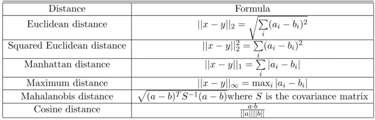
Distance Formula Euclidean distance ||x−y||2 =√∑
i
(ai−bi)2
Squared Euclidean distance ||x−y||22 =∑
i (ai−bi)2 Manhattan distance ||x−y||1 = ∑ i |ai−bi|
Maximum distance ||x−y||∞= maxi|ai−bi|
Mahalanobis distance √(a−b)TS−1(a−b)whereS is the covariance matrix
Cosine distance ||aa||||·bb|| Table 2.1: Distance measurement.
2.2
Overview of Clustering Algorithms
Clustering is an unsupervised data pattern extraction process that aims at grouping similar patterns into the same category based on certain measures of “distance” [4]. Cluster analysis aims to discover clusters or groups of samples such that samples within the same group are more similar to each other than they are to the samples of other groups. It is a kind of statistical data analysis widely used in many fields, including Machine Learning, Data Mining. It has led to the design and analysis of a wide spectrum of algorithms.
When talking about clustering, a distance measurement is needed to represent the close-ness of two points. Commonly used distance of measurements are listed in Table. 2.1. In this thesis, Euclidean distance is used as the default measurement if not otherwise noted.
The similarity matrix (also known as Gram matrix or G-matrix) is a matrix of scores which expresses the similarity between data points. Let{Xi}Ni=1be a set of points inRD (D
is the dimensionality), the similarity matrix is anN ×N matrix, the (i, j)th entry is given by
Sij =||Xi−Xj||2, (2.1)
where (||expressions||2 stands for L2 distance or Euclidean distance).
Similarity matrix plays a crucial role in kernel-based methods. Techniques such as linear Support Vector Machines (SVM) Gaussian Processes [32] can only extract structure from the original dataset by computing linear functions, e.g., functions in the form of dot products. When there are nonlinear structures in the data, the above mentioned linear techniques will
lose effectiveness [15]. Kernel-based learning methods have proved to be useful in the above mentioned scenarios [15]. For instance, in kernel-based SVM [15], data items are mapped into high-dimensional space, where information about their mutual positions (in the form of inner products) is used for constructing classification, regression, or clustering rules. Kernel-based algorithms exploit the information encoded in the inner product between all pairs of data items and are successful in part because there is often an efficient method to compute inner products between very complex or even infinite dimensional vectors. Thus, kernel-based algorithms provide a way to deal with nonlinear structure by reducing nonlinear algorithms to algorithms that are linear in some feature space that is nonlinearly related to the original input space. Moreover, Similarity matrices are also widely used in sequence alignment in biomedical studies [24]. Higher scores are given to more-similar characters, and lower or negative scores for dissimilar characters. Nucleotide similarity matrices are used to align nucleic acid sequences [24].
There are several genres of clustering algorithms. In the following sections, we introduce some important classes and explain how they can be implemented in a distributed manner.
2.3
Hierarchical Clustering Algorithms
Hierarchical algorithms [10] find successive clusters using previously established clusters. These algorithms usually are either agglomerative (bottom-up) or divisive (top-down). Ag-glomerative algorithms begin with each element as a separate cluster and merge them into successively larger clusters. Divisive algorithms begin with the whole set and proceed to divide it into successively smaller clusters.
For agglomerative approach, given a set of N points to be clustered, and an N ×N
distance (or similarity) matrix, the process of hierarchical clustering is as follows:
• Step 1: Start by assigning each item to its own cluster, so that if we haveN items, we now haveN clusters, each containing just one item. Let the distances (similarities) between the clusters equal the distances (similarities) between the items they contain.
• Step 2: Find the closest (most similar) pair of clusters and merge them into a single cluster, so that now we have one less cluster.
• Step 3: Compute distances (similarities) between the new cluster and each of the old clusters.
• Step 4: Repeat steps 2 and 3 until all items are clustered into a single cluster of size
N.
Step 3 can be done in different ways, which is what distinguishes single-link from complete-link and average-link clustering. In single-link clustering [10], we consider the distance between one cluster and another cluster to be equal to the shortest distance from any member of one cluster to any member of the other cluster. If the data consist of similarities, we consider the similarity between one cluster and another cluster to be equal to the greatest similarity from any member of one cluster to any member of the other cluster. In complete-link clustering [10], we consider the distance between one cluster and another cluster to be equal to the longest distance from any member of one cluster to any member of the other cluster. In average-link clustering, we consider the distance between one cluster and another cluster to be equal to the average distance from any member of one cluster to any member of the other cluster.
It is inefficient to apply the agglomerative model to MapReduce, because each distributed task needs the entire dataset to make choices about appropriate clusters. It also needs a list of clusters at its current level such that it does not add a data point to more than one cluster at the same level. This is a class of applications that is unsuitable for MapReduce [62].
2.4
Partitional Clustering Algorithms
Partitional algorithms typically determine all clusters at once, and can also be used as divisive algorithms in the hierarchical clustering described in Section 2.3.
2.4.1 K-means
K-means [27] follows a simple and easy way to classify a given dataset through a certain number of clusters (assume k clusters fixed as a priori). The main idea is to define k
centroids, one for each cluster. These centroids should be placed in a clever way, because different location causes different result. Therefore, a good choice is to place them as much as possible far away from each other. The next step is to take each point belonging to a given dataset and associate it to the nearest centroid. When no point is pending, the first step is completed and an early clustering is done. At this point we need to re-calculate
k new centroids as centers of the clusters resulting from the previous step. After we have these knew centroids, a new binding has to be done between the same dataset points and the nearest new centroid. A loop has been generated. As a result of this loop we may notice that the kcentroids change their location step by step until no more changes are done. In other words centroids do not move any more.
This algorithm aims at minimizing an objective function, in this case a squared error function. The objective function is:
J = k ∑ j=1 N ∑ i=1 ||x(ij)−cj||2, (2.2)
where||x(ij)−cj||2is a chosen distance measure between a data pointx(ij)and the cluster
centercj, the algorithm is composed of the following steps:
• Step 1: Place k points into the space represented by the objects that are being clustered. These points represent initial group centroids.
• Step 2: Assign each point to the group that has the closest centroid.
• Step 3: Recalculate the positions of the k centroids when all points have been as-signed.
• Step 4: Repeat Steps 2 and 3 until the centroids no longer move. This produces a separation of the points into groups from which the objective function to be minimized can be calculated.
A MapReduce parallel algorithm for K-means clustering has been proposed by Zhao et al. [49]. Initially k points are chosen as the cluster centers. Each map function gets a partition of the data and accesses this partition in each iteration. The variable data is the current cluster centers calculated during the previous iteration, hence it is used as the input value for the map function. All the map functions get this same input data (current cluster centers) at each iteration and computes partial cluster centers by going through its dataset. Note that each map function can identify the nearest cluster for its data points because it has access to all cluster centers. Thus, each map function is able to update the cluster membership for its data points. A reduce function computes the average of all points for
each cluster based on the updated membership and produces the new cluster centers for the next step. Once it gets these new cluster centers, it calculates the difference between the new cluster centers and the previous cluster centers and determines if it needs to execute another cycle of MapReduce computation.
2.4.2 Affinity Propagation
Frey and Dueck present an algorithm called affinity propagation [22] which clusters data points via passing messages between the points. Affinity propagation clusters data by diffu-sion in the similarity matrix. Input consists of a collection of real-valued similarities between data points. These are represented bys(i, k) which describes how well data pointkis suited to be exemplar for data pointi. In addition, each data point is supplied with a preference values(k, k) which specifies a priori on how likely each data point is to be an exemplar.
There are two kinds of messages exchanged between data points, responsibilities and availabilities. Responsibility r(i, k) reflects the accumulated evidence for how well-suited pointkis to serve as the exemplar for pointi, taking into account other potential exemplars for pointi. Responsibility is sent from pointito candidate exemplar k. Availabilitya(i, k) reflects accumulated evidence for how appropriate it would be for point i to choose k as its exemplar, taking into account the support from other points that pointk should be an exemplar. Availability is sent from candidate exemplar k to data point i. In general the algorithm works in three steps:
• Update responsibilities given availabilities. Initially this is a data driven update. Over time it lets candidate exemplars compete for ownership of the data.
• Update availabilities given the responsibilities. This gathers evidence from data points as to whether a candidate exemplar is a good exemplar.
• Monitor exemplar decisions by combining availabilities and responsibilities. Terminate if reaching a stopping point (e.g. insufficient change). The update rules require simple local computations and messages are exchanged between pairs of points with known similarities.
The update is done according to the following formulas:
r(i, k) = (1−λ)×r(i, k) +λ×(s(i, k)− max
k′:k′̸=k(a(i, k
′) +s(i, k′))),
a(i, k) = (1−λ)×a(i, k) +λ×min{0, r(k, k) + ∑ i′:i′̸⊂i,k max(0, r(i′, k))}, (2.4) a(k, k) = (1−λ)×a(k, k) +λ× ∑ i′:i′̸=k max(0, r(i′, k)), (2.5)
whereλis the damping factor used to avoid numerical oscillations.
We can see from the above formulas, in every iteration, it involves both row scan and column scan, therefore, it is impossible to parallelize the whole process use MapReduce. One possible method is to parallelize r matrix calculation and a calculation separately in a single loop. Wang et al. [60] propose a method to parallelize Affinity propagation. To parallelize r(i, k), all the values of a(i, k′) and s(i, k′) are taken as map input. In reduce part, all the values takingias key are passed into the reduce function as a list. To parallelize
a(i, k), all the values ofr(i′, k) are taken as input, since all the key/value pairs are indexed by the column afterr(i, k) calculation, all the values in the k-th column are organized as a list.
2.5
Soft Clustering Algorithms - Dirichlet Process Clustering
(DPC)
“Soft”, in this context, means that a point can fall into two (or more than two) clusters. The algorithms in this genre use probabilistic generative models. Dirichlet Process Clustering (DPC) [7] falls into this genre.
The calculation goes in an iterative manner. There are mainly three steps in each iteration [7]:
• Assign the input data points to a certain cluster.
• Update the model by computing the posterior probabilities and new model parameters by sampling from a Dirichlet distribution.
One way of parallelizing DPC using MapReduce framework is described in [49]. In every iteration, there are map and reduce functions. In map function, it assigns the input data points to a certain cluster, then emits the pair< pointID, clusterID >. In reduce function, it updates the models by computing the posterior probabilities and new model parameters. Then it emits the pair as the output of this iteration. This loop goes for a predefined iterations.
2.6
Spectral Clustering
Spectral Clustering [46] is a class of methods based on eigen decomposition of affinity, dissimilarity or kernel matrices [46]. Many clustering methods are strongly tied to Euclidean distance, making assumptions that clusters form convex regions in Euclidean space. Spectral methods are more flexible, capturing a wider range of geometries. Spectral Clustering is widely used in Document Clustering [66], Image Segmentation [61]. Moreover, there is a substantial theoretical literature supporting Spectral Clustering [46].
The idea of Spectral Clustering is to form a pairwise similarity matrix S, compute Laplacian matrixLand compute eigenvectors ofL. It is shown that the second eigenvector of the normalized graph Laplacian is a relaxation of a binary vector solution that minimizes the normalized cut on a graph [46].
Given a set of points {Xi}Ni=1 in Rd (d is the dimensionality), The algorithm proceeds
as follows:
• Step 1: Form the similarity matrix S ∈ RN×N defined by Sij = exp(−||Xi −
Xj||2/2σ2) if i̸=j, and Sii= 0.
• Step 2: Define D to be the diagonal matrix whose (i, i)-element is the sum of S’s
i-th row, and construct the matrix L=D−1/2AD−1/2.
• Step 3: Find V1, V2..., Vk, the top k eigenvectors of L, and form the matrix X =
[V1V2...Vk]∈RN×k by stacking the eigenvectors in columns.
• Step 4: Form the matrixY from X by renormalizing each of X’s rows to have unit length, Yij =Xij/(
√∑
j
X2 ij).
• Step 5: Treat each row of Y as a point in Rk, cluster them into k clusters using K-means [27].
• Step 6: Assign the original point Xi to cluster j if and only if rowiof the matrix Y
is assigned to cluster j.
The scaling parameterσ2controls how rapidly the affinitySijdecreases with the distance
betweenXi andXj. The eigenvectors of a square matrix are the non-zero vectors that, after
being multiplied by the matrix, remain parallel to the original vector. For each eigenvector, the corresponding eigenvalue is the factor by which the eigenvector is scaled when multiplied by the matrix.
The advantages of Spectral Clustering can be summarized as follows:
• Spectral Clustering performs well with non-Gaussian clusters [46].
• As opposed to K-means clustering, which results in convex sets, Spectral Clustering can solve problems such as intertwined spirals, because it does not make assumptions on the form of the cluster. This property comes from the mapping of the original space to an eigen space.
• Spectral Clustering does not intrinsically suffer from the problem of local optima [46]. Spectral Clustering performs significantly better than the linkage algorithm [41] even when the clusters are not well separated.
Spectral Clustering is parallelized in MapReduce framework [49]. In Laplacian matrix computing part, since it involves matrix multiplication, the parallelization computes each entry in Laplacian matrix separately and reduces the results into one single matrix. In the K-means clustering part, it is parallelized in a way that is introduced in Section 2.4. Spectral Clustering has also been parallelized using MPI by Chen et al. [13].
2.7
Challenges in Clustering Large Datasets
Clustering large-scale datasets using kernel-based methods is challenging. The difficulties are summarized into three folds:
• The similarity matrix, on which many kernel-based clustering algorithms rely, needs
O(N2) complexity in time to compute. When running on large datasets, it can be intolerably long.
• The similarity matrix needs O(N2) memory space to store. Although the state-of-art high performance computers have very large DRAM, when applying large datasets, the memory will still be insufficient and thrashing is likely to occur in the paging system, which make the running process even slower.
• Most of the clustering algorithms suffer from “curse of dimensionality” [23] that comes with high-dimensionality data. Essentially, the amount of data to sustain a given spa-tial density increases exponenspa-tially with the dimensionality of the input space, or alternatively, the sparsity increases exponentially given a constant amount of data, with points tending to become far apart from one another. In general, this will ad-versely impact any method based on spatial density, unless the data follows certain simple distributions.
2.8
Related Work
Clustering large datasets is an actively researched area [68] [12] [36]. For example, Kulis and Grauman [36] target large-scale scalable image search. They generalize locality-sensitive hashing to accommodate arbitrary kernel functions, therefore permitting sub-linear time approximate similarity search. Another example is BIRCH [68], which is a method for pre-clustering large datasets. BIRCH incrementally groups the data as tightly as possible based on similarity in their attributes. In the process, it constructs as many representatives of the original data as the available memory can contain. If the amount of space taken by the data runs out during the BIRCH process, the tightness of the groupings is relaxed, the groupings are internally re-assigned, and the processing of the data continues. Therefore, by monitor-ing the system’s available memory, BIRCH can dynamically adjust the clustermonitor-ing policies. Chen and Liu [12] propose “iVIBRATE”, which is an interactively visualization based three-phase framework for clustering large datasets. Two main components of iVIBRATE are its visual cluster rendering subsystem, which enables human to join the large-scale iterative clustering process through interactive visualization, and its Adaptive ClusterMap Label-ing subsystem, which offers visualization-guided disk-labelLabel-ing solutions that are effective in dealing with outliers, irregular clusters, and cluster boundary extension. However, when presented with high-dimensional large-scale datasets, the visual presentation will not work because of human’s incapability of high-dimensional data perception.
dimensionality is typically addressed by feature selection and dimension reduction techniques [56]. Radovanovic et al. [53] study the number of times a point appears among theknearest neighbors of other points in a dataset. They identify that, as dimensionality increases, this distribution becomes considerably skewed and points with very high occurrences emerge. This is a new property that is discovered in high-dimensional datasets. Murtagh et al. also explore hierarchical clustering on high-dimensional datasets using ultrametric embedding [44]. An ultrametric is a metric which satisfies the following triangle inequality: d(x, z) ≤ max(d(x, y), d(y, z)) for all points x,y and z. By quantifying the degree of ultrametricity [3] in a dataset, Bartal et al. show that ultrametricity becomes pervasive as dimensionality and/or spatial sparsity increases.
Clustering optimization for specific applications has also been studied. For example, in [40], Manku utilizes simHash [11] to generate a signature for each web page and then separate web-scale dataset apart into different buckets. However, their work is optimized for a specific application and is potentially difficult to generalize, while our work is designed to fit the majority of main stream kernel-based clustering algorithms.
Research on speeding up the execution of Spectral Clustering can be summarized in two directions. One direction is subsampling approach, selecting data points following some form of stratification procedure. One of the best known approximation schemes is sampling using the Nystrom method [63]. This method allows extrapolation of the complete grouping solution using only a small number of typical samples. Fowlkes et al. [21] propose using the Nystrom extension to approximate the eigenvectors of the affinity matrix. They investigate the Nystrom extension solution to the Normalized Cut problem [46] in Spectral Clustering and apply the method in image segmentation. In [57], Schuetter et al. extend the above mentioned method and propose a multiple subsample approach that improves the accuracy of the Nystrom extension.
The other direction is approximating the affinity matrix. Cullum and Willoughby [16] introduce the Lanczos algorithm, which uses a sparse eigensolver to do the decomposition. Matrix sparsity can be created by computing entries for only those elements within an ϵ -neighborhood of each other, or for nearest neighbors. However, this method still runs in
O(N2) time. Drineas et al. [19] develop an algorithm to compute a low-rank approximation to similarity matrix. The low-rank approximation problem is to approximate a matrix by one of the same dimension but smaller rank with respect to some norm, e.g., the Frobenius norm. They use a data-dependent nonuniform probability distribution to randomly sample
the columns.
We identify two recent works that are close to ours [64] [13]. Yan et al. [64] propose leveraging K-means to pre-process the original datasets and pre-group them. Although we share the same rationale, as shown later in the thesis, our method can be applied to many clustering algorithms beyond the Spectral Clustering algorithm. Also, the method in [64] does not consider the complexity when partitioning the original dataset. On the contrary, our method can achieveO(N) when doing the partitioning step, and the constant factor inO(N) is small. Chen et al. [13] propose parallel Spectral Clustering method that approximates the affinity matrix and compare it against the Nystrom extension method. The method forms the sparse matrix via retaining a group of nearest neighbors. To retain nearest neighbors, for every point in the dataset, the method computes the similarity between this point and others. It keeps a heap to retain the closest points. The method is essentially a variation ofk-nearest neighbor search [46]. The advantage of the method is small memory footprint. However, the method still has to compute the similarity for every pair of points, thus its time complexity remains unchanged at O(N2). On the contrary, our method can achieve O(N) complexity in the preprocessing step with MapReduce framework, and it only computes the similarity values between a subset of data points instead of all points. Therefore, the proposed method can achieve sub-quadratic complexity in both time and space.
We compare the proposed method, which we call distributed Spectral Clustering (DASC) against three existing methods: the original Spectral Clustering algorithm (denoted asSC) [46], Parallel Spectral Clustering (denoted asP SC) [13] and Nystrom approximation method (denoted asN Y ST) [21]. SC serves as the baseline comparison,P SCuses nearest-neighbor-search to reduce the size of similarity matrix and is parallelized using MPI, andN Y ST is a recently proposed scheme which leverages K-means to pre-group neighboring points and produces a set of reduced representative points for Spectral Clustering.
Proposed Distributed Spectral
Clustering Algorithm
3.1
Overview
Kernel-based clustering techniques perform computation based on similarity matrix. In or-der to reduce the complexity of this expensive operation, which is O(N)2 where N is the dataset size, we propose a preprocessing step using Locality Sensitive Hashing to approx-imate the similarity matrix. In the similarity matrix, every element reflects the similarity between two points. The larger the element is, the closer those two points are. In the proposed algorithm, those small elements in the original similarity matrix will not be com-puted and they will be omitted. The proposed method decides whether or not to compute an element in similarity matrix using Locality Sensitive Hashing [43]. Every point in the dataset is labeled with a signature, identical or similar signatures mean that the correspond-ing points are close to each other, thus their similarity value is large. Big difference between two signatures means that the corresponding points are far away from each other, thus they are unlikely to be in the same cluster and their similarity value is small. Therefore, we do not compute similarity for such two points.
There are several steps in the proposed algorithm. In the first step, the algorithm iterates through the dataset once to generate signatures. In the second step, points whose signatures are similar to each other are projected into one bucket. In the third step, similarity values are computed for the points in each bucket to form the approximated matrix. In the fourth
step, Spectral Clustering algorithm will run on the approximated similarity matrix and output the clustering results.
In the following sections, we will first review different families of Locality Sensitive Hashing and then describe the proposed algorithm and implementation details.
3.2
Locality Sensitive Hashing
Locality Sensitive Hashing (LSH) is a probabilistic dimension reduction technique [43]. The idea is to hash points such that the probability of collision is much higher for close points than for those that are far apart. Those points whose hashing values collide with each other fall into the same bucket. Then, one can determine nearby neighbors by hashing the query point and retrieving elements stored in buckets containing that point.
For a domainSof the points set with distance measurementD, an LSH family is defined as follows [43].
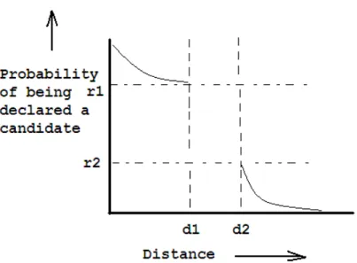
Definition 1 (LSH Family) A family H ={h:S →U} is called (d1, d2, p1, p2)-sensitive for D if for anyx, y∈S, we have:
• if x∈B(y, d1) thenP rH[h(x) =h(y)]≥p1,
• if x̸∈B(y, d2) thenP rH[h(x) =h(y)]≤p2,
where p1 > p2, d1 < d2, and B(y, d) is square area centered at y with radius d. The
behavior is shown in Fig. 3.1.
3.2.1 Stable Distributions
According to [47], a distribution is a stable distribution if it satisfies the following property: LetX1 and X2 be independent copies of a random variable X. Random variable X is said
to be stable if for any constants a and b the random variable a·X1+b·X2 has the same
distribution asc·X+dwith some constantscand d. The distribution is said to be strictly stable if this holds withd= 0.
A distribution D over R is called p−stable, if there exists p ≥ 0 such that for any
n real numbers v1, ..., vn and independent identically distributed variables X1, ..., Xn with
distribution D, the random variable ∑
i
vi ·Xi has the same distribution as the variable
(∑
i
Figure 3.1: Behavior of a (d1, d2, p1, p2)-sensitive function. In the case of RD withL2 distance, p-stable distribution is defined as:
H(v) =< h1(v), h2(v), ..., hM(v)>, (3.1)
hi(v) =⌊
ai·vi+bi
W ⌋, i= 1,2, ..., M, (3.2)
whereai ∈RD is a vector with entries chosen independently from the Gaussian
distribu-tionN(0,1) andbi is drawn from the uniform distribution U[0, W). For different i,ai and
bi are sampled independently. The parameters M and W control the locality sensitivity of
the hash function.
3.2.2 Random Projection
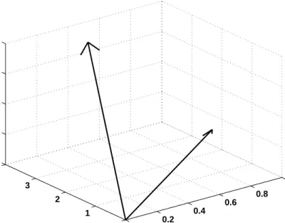
The random projection method [9] is designed to approximate the cosine distance between vectors. The idea of this technique is to choose a random hyperplane (defined by a normal unit vectorr) at the outset and use the hyperplane to hash input vectors.
0 0.2 0.4 0.6 0.8 1 0 1 2 3 4 0 0.5 1 1.5 2
Figure 3.2: Two vectors in three dimensions making an angle.
Given two vectorsx andy, the cosine of the angle between them is the dot productx·y
divided by theL2−normofxandy, for instance, their Euclidean distances from the origin.
In Figure 3.2, it can be observed that two vectorsxandymake an angleθbetween them. It should be noted that the vectors may be in a many-dimension-space, however, they always define a plane, and the angle between them is measured in this plane. Given an input vector
v and a hyperplane defined by r, we let h(v) = sgn(v·r) = ±1. Each possible choice of r
defines a single function. LetH be the set of all such functions and let D be the uniform distribution. For two vectorsu,v, we have:
P r[h(u) =h(r)] = 1−θ(u, v)
π , (3.3)
whereθ(u, v) is the angle betweenu and v.
Givenm functions in this family, there will be mbits in the result for every input data point. Thesem bits are concatenated and serve as a unique signature for the input vector. Points having a large portion of corresponding bits identical are considered to be close to each other.
3.2.3 Summary of Locality Sensitive Hashing
Besides what is covered above, there are other Locality Sensitive Hashing families. For instance, Min-Wise Independent Permutations [14], which uses Jaccard Index [33] to group similar documents together. The documents do not contain explicit numerical features. Locality Sensitive Hashing for Hamming distance operates on binary sequences when the input points live in the Hamming space. For p-stable distribution, Equation (3.2) essen-tially projects a multi-dimensional vector onto one-dimensional space. We need to tune the parameters bi, W and M in Equation (3.2) based on the data characteristics. Also, the
basic Locality Sensitive Hashing index requires large W,M to satisfy certain recall. This trades space for fast query time. The hash function we use to generate the signatures falls into the family of Random Projection. The advantage of this family is that, after applying hashing function once, we only need one bit to store the result. This characteristic saves a lot of storage space. It has been shown that Random Projection has the best performance in high-dimensional data clustering [20]. Also, with Random Projection, we can compare the generated signatures using hamming distances for which efficient algorithms are available [11].
3.3
Distributed Approximate Spectral Clustering
The proposed algorithm approximates the similarity matrix, speeds up the execution of kernel-based clustering techniques and reduce the memory footprint. Moreover, it can be parallelized easily using MapReduce framework.
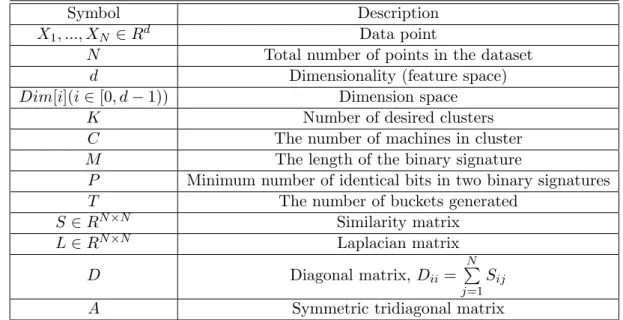
For quick reference, we list all symbols used in this chapter in Table 3.1.
The approximation scheme goes in the following steps, Step 3 toStep 8 are the steps in Spectral Clustering:
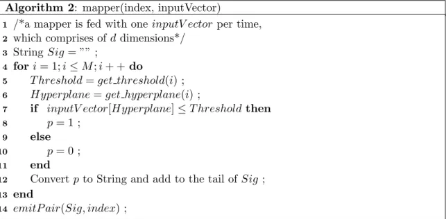
• Step 1: Create signatures for data points. Every point in the dataset is represented by an index and a group of numerical features. The signature is anM-bit string, each bit is generated as follows: one feature in the dimensionality space is selected. This feature is then compared with a threshold. If the feature is larger than thethreshold, the resulting bit is set to 1, otherwise it is set to 0. This process goes M times, and the resulting bits are concatenated to make the signature. The complexity of this step is O(M·N). This hash function falls into Random Projection family, because every
Symbol Description
X1, ..., XN ∈Rd Data point
N Total number of points in the dataset
d Dimensionality (feature space)
Dim[i](i∈[0, d−1)) Dimension space
K Number of desired clusters
C The number of machines in cluster
M The length of the binary signature
P Minimum number of identical bits in two binary signatures
T The number of buckets generated
S ∈RN×N Similarity matrix L∈RN×N Laplacian matrix D Diagonal matrix, Dii= N ∑ j=1 Sij
A Symmetric tridiagonal matrix
Table 3.1: List of symbols used in this chapter.
time we apply this hash function, we project all the points in a dataset onto a line. After that, the hashing result is determined by comparing the projection value against a threshold.
• Step 2: All points that have near-duplicate signatures are projected into one bucket. Near-duplicate signatures mean that for twoM-bit binary numbers, there are at least
P bits in common. Suppose the total number of different signatures generated is T, the complexity of this step isO(T2).
• Step 3: Compute the sub similarity matrix in every bucket. Suppose we have alto-gether T different signatures, we then have T buckets, each of which has Ni (where
0≤i≤T−1 and
T∑−1 i=0
Ni =N) points, the overall complexity of this step is T∑−1
i=0
O(Ni2). The similarity function is:
Sij =exp(−||
Xi−Xj||2
2σ2 ), (3.4)
where σ is a scaling parameter to control how rapidly the similarity Sij reduces with
• Step 4: Construct the Laplacian matrix for each sub similarity matrixSi inStep 3:
Li=Di−1/2SiD−i 1/2, (3.5)
where D−i 1/2 is the inverse square root of Di, Di is diagonal matrix. For an Ni×Ni
diagonal matrix, the complexity of finding inverse square root is O(Ni). Moreover,
the complexity of multiplying an Ni×Ni diagonal matrix with anNi×Ni matrix is
O(Ni2). Therefore, the complexity of this step is O(
T∑−1 i=0
Ni2).
However, if the similarity matrix is sparse, the actual running time can be greatly reduced, as we can skip the computation of zero entries in similarity matrix. For a similarity matrix that contains U non-zero entries, the complexity of multiplying it with a diagonal matrix is O(U).
• Step 5: Find V1, V2..., VKi, the first Ki eigenvectors of Li, and form the matrix
Xi = [V1V2...VKi]∈ R
Ni×Ki by stacking the eigenvectors in columns. To do this, we
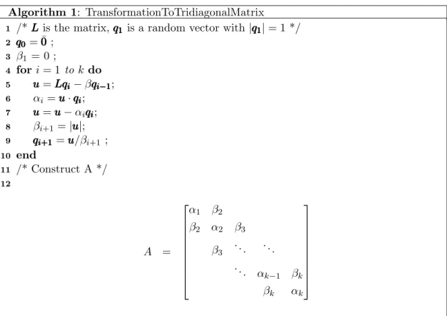
first transformLi into a symmetric tridiagonal matrixKi×KiAi. The transformation
routine is shown in Fig. 3.3. The tridiagonal matrixAiis constructed using the derived
αi and βi (i∈[1, Ki]) in Fig. 3.3.
The complexity of the transformation is Ki ·Ni. However, if Li is a sparse matrix,
the actual running time can be greatly reduced, as we can skip the computation of zero entries. This transformation preserves the eigenvectors and the eigenvalues of the original matrix, and can greatly speed up the following QR decomposition [16]. Specifically, QR decomposition on a tridiagonal matrix has complexity of O(Ki), in
contrast, QR decomposition on a general matrix is O(Ki3) [52].
Following this, we do eigen decomposition on Ai using QR decomposition, as
men-tioned above, the complexity is O(Ki). Therefore, the total complexity of this step is
O(
T∑−1 i=0
(Ki·Ni)).
• Step 6: Form the matrixY from X by renormalizing each of X’s rows to have unit length, Yij =Xij/(√∑
j
Algorithm 1: TransformationToTridiagonalMatrix
/*LLLis the matrix,qqq111 is a random vector with|qqq111|= 1 */
1 qqq000 = ¯000 ; 2 β1 = 0 ; 3 fori= 1 tok do 4 u uu=LLLqqqiii−βqqqiii−−−111; 5 αi =uuu·qqqiii; 6 u uu=uuu−αiqqqiii; 7 βi+1 =|uuu|; 8 qi+1 qqii+1+1 =uuu/βi+1 ; 9 end 10 /* Construct A */ 11 12 A = α1 β2 β2 α2 β3 β3 . .. . .. . .. αk−1 βk βk αk
• Step 7: Treat each row of Y as a point in RKi, cluster them into K
i clusters using
K-means [27]. The complexity of this step isO(
T∑−1 i=0
(Ki·Ni)).
• Step 8: Assign the original point Xi to cluster j if and only if rowiof the matrix Y
is assigned to cluster j. The complexity of this step isO(N).
After Step 1 and Step 2, points in every bucket run Spectral Clustering (from Step 3 toStep 8). Therefore, the total complexity of the proposed algorithm is:
T imeComplexity=O(M ·N) +O(T2) + T∑−1 i=0 [ 2·O(Ni2) + 2·(Ki·Ni) ] + 2·N. (3.6) The hyperplane value and threshold value are important factors in the hash function. The threshold value controls at which threshold we separate the original dataset apart, the hyperplane value controls which feature space to compare with the corresponding threshold. We use the principle of k-dimensional tree (k-d tree) [35] to set hyperplane value and thresh-old value. The k-d tree is a binary tree in which every node is a k-dimensional point. Every non-leaf node can be thought of as implicitly generating a splitting hyperplane that divides the space into two parts, known as subspaces. Points to the left of this hyperplane are rep-resented by the left subtree of that node and points right of the hyperplane are reprep-resented by the right subtree. The hyperplane direction is chosen in the following way: every node in the tree is associated with one of the k-dimensions, with the hyperplane perpendicular to that dimension’s axis. For example, if for a particular split the “x” axis is chosen, all points in the subtree with a smaller “x” value than the node will appear in the left subtree and all points with larger “x” value will be in the right subtree. In such a case, the hyperplane would be set by the x-value of the point, and its normal would be the unit x-axis.
To determine the hyperplane array, we look at each dimension of the dataset, and calculate the numerical span for all the dimensions (denoted asspan[i], i∈[0, d)). Numerical span is defined as the difference of the largest value and the smallest value in this dimension. For example, in Dim[j], the largest value is 0.9 and the smallest value is 0.1, then the numerical span associated with this dimension is 0.8. We then rank the dimensions according to their numerical spans. The possibility of one hyperplane[i] being chosen by the hash function is proportional to:
prob=span[i]/
d−1
∑
i=0
span[i]. (3.7)
This is to ensure dimensions with large span have more chance to be selected. More analysis can be found in Sec. 3.6.
For each dimension space Dim[i], the associated threshold is determined as follows: between the minimum (denoted asmin[i]) and maximum (denoted asmax[i]) inDim[i], we create 20 bins (denoted as bin[j], j ∈[0,19]), bin[j] will count the number of points whose
i−th dimension fall into the range [min[i] +j×span[i]/20, min[i] + (j+ 1)×span[i]/20). We then find out the minimum in array bin (denoted as bin[s]), the threshold associated withDim[i] is set toDim[i] =min[i] +s×span[i]/20.
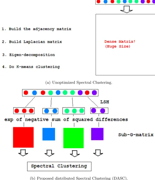
Fig. 3.4(a) illustrates the scenario when we compute the similarity matrix from the original dataset without approximation. Since both space complexity and time complexity of computing the similarity matrix areO(N2) for a dataset containingN points, the similarity
matrix will take too much time to compute. The failure of computing similarity matrix will render Spectral Clustering unfeasible to run. Our proposal is illustrated in Fig. 3.4(b): add a pre-processing step on top of similarity matrix computation to separate the raw dataset apart into several buckets according to their proximity and locality measurements. Then, build the similarity matrix separately for each partition of data.
3.4
MapReduce Implementation of DASC Algorithm
MapReduce [18] is a programming model for writing applications that can rapidly process vast amount of data in parallel on a cluster. Hadoop [62] is an open source implementation of MapReduce. Hadoop makes it possible to run applications on systems with thousands of nodes, these nodes can be of different computing power. We present the design of the proposed DASC algorithm using the MapReduce programming model and we implement it in the opensource Hadoop platform. A MapReduce job is a unit of work to be performed: it consists of the input data, the MapReduce program, and configuration information. Hadoop runs the job by dividing it into tasks. There are two types of tasks: map tasks and reduce tasks.
(a) Unoptimized Spectral Clustering.
(b) Proposed distributed Spectral Clustering (DASC).