Querying Data Provenance

(1)

University of Pennsylvania

ScholarlyCommons

Departmental Papers (CIS)

Department of Computer & Information Science

6-2010

Querying Data Provenance

Grigoris Karvounarakis

LogicBox

Zachary G. Ives

University of Pennsylvania

, zives@cis.upenn.edu

Val Tannen

University of Pennsylvania

, val@cis.upenn.edu

Follow this and additional works at:

http://repository.upenn.edu/cis_papers

Part of the

Computer Sciences Commons

Karvounarakis, G., Ives, Z., & Tannen, V., Querying Data Provenance,ACM SIGMOD International Conference on Management of Data, June 2010, doi:

10.1145/1807167.1807269

ACM COPYRIGHT NOTICE. Copyright © 2010 by the Association for Computing Machinery, Inc. Permission to make digital or hard copies of part or all of this work for personal or classroom use is granted without fee provided that copies are not made or distributed for profit or commercial advantage and that copies bear this notice and the full citation on the first page. Copyrights for components of this work owned by others than ACM must be honored. Abstracting with credit is permitted. To copy otherwise, to republish, to post on servers, or to redistribute to lists, requires prior specific permission and/or a fee. Request permissions from Publications Dept., ACM, Inc., fax +1 (212) 869-0481, orpermissions@acm.org. This paper is posted at ScholarlyCommons.http://repository.upenn.edu/cis_papers/621

For more information, please contactlibraryrepository@pobox.upenn.edu.

Recommended Citation

(2)

Querying Data Provenance

Abstract

Many advanced data management operations (e.g., incremental maintenance, trust assessment, debugging

schema mappings, keyword search over databases, or query answering in probabilistic databases), involve

computations that look at how a tuple was produced, e.g., to determine its score or existence. This requires

answers to queries such as, “Is this data derivable from trusted tuples?”; “What tuples are derived from this

relation?”; or “What score should this answer receive, given initial scores of the base tuples?”. Such questions

can be answered by consulting the provenance of query results. In recent years there has been significant

progress on formal models for provenance. However, the issues of provenance storage, maintenance, and

querying have not yet been addressed in an application-independent way. In this paper, we adopt the most

general formalism for tuple-based provenance, semiring provenance. We develop a query language for

provenance, which can express all of the aforementioned types of queries, as well as many more; we propose

storage, processing and indexing schemes for data provenance in support of these queries; and we

experimentally validate the feasibility of provenance querying and the benefits of our indexing techniques

across a variety of application classes and queries.

Disciplines

Computer Sciences

Comments

Karvounarakis, G., Ives, Z., & Tannen, V., Querying Data Provenance,

ACM SIGMOD International Conference

on Management of Data

, June 2010, doi:

10.1145/1807167.1807269

ACM COPYRIGHT NOTICE. Copyright © 2010 by the Association for Computing Machinery, Inc.

Permission to make digital or hard copies of part or all of this work for personal or classroom use is granted

without fee provided that copies are not made or distributed for profit or commercial advantage and that

copies bear this notice and the full citation on the first page. Copyrights for components of this work owned

by others than ACM must be honored. Abstracting with credit is permitted. To copy otherwise, to republish,

to post on servers, or to redistribute to lists, requires prior specific permission and/or a fee. Request

permissions from Publications Dept., ACM, Inc., fax +1 (212) 869-0481, or

permissions@acm.org

.

(3)

Querying Data Provenance

Grigoris Karvounarakis

∗

LogicBlox ICS-FORTH

Atlanta, GA, USA Heraklion, Greece

gregkar@gmail.com

Zachary G. Ives

Val Tannen

University of Pennsylvania Philadelphia, PA, USA

{zives,val}@cis.upenn.edu

ABSTRACT

Many advanced data management operations (e.g., incremental main-tenance, trust assessment, debugging schema mappings, keyword search over databases, or query answering in probabilistic databases), involve computations that look at how a tuple was produced, e.g., to determine its score or existence. This requires answers to queries such as, “Is this data derivable from trusted tuples?”; “What tuples are derived from this relation?”; or “What score should this answer receive, given initial scores of the base tuples?”. Such questions can be answered by consulting theprovenanceof query results.

In recent years there has been significant progress on formal models for provenance. However, the issues of provenance stor-age, maintenance, and querying have not yet been addressed in an application-independent way. In this paper, we adopt the most gen-eral formalism for tuple-based provenance,semiring provenance. We develop a query language for provenance, which can express all of the aforementioned types of queries, as well as many more; we propose storage, processing and indexing schemes for data prove-nance in support of these queries; and we experimentally validate the feasibility of provenance querying and the benefits of our index-ing techniques across a variety of application classes and queries.

Categories and Subject Descriptors

H.2.3 [Database Management]: Languages—Query languages; H.2.4 [Database Management]: Systems—Query processing

General Terms

Languages, Performance, Algorithms

Keywords

Data provenance, annotation, query language, query processing

1. INTRODUCTION

In the sciences, in intelligence, in business, the same adage holds true: data is only as credible as its source. Recently we have be-gun to see issues like data quality, uncertainty, and authority make

∗_{Work performed while the first author was a Ph.D. candidate at}

the University of Pennsylvania.

Permission to make digital or hard copies of all or part of this work for personal or classroom use is granted without fee provided that copies are not made or distributed for profit or commercial advantage and that copies bear this notice and the full citation on the first page. To copy otherwise, to republish, to post on servers or to redistribute to lists, requires prior specific permission and/or a fee.

their way from separate data processing stages, into the very foun-dations of database systems: data models, mapping definitions, and query languages. Typically, the notion ofdata provenance[12, 18, 29] lies at the heart of assessing authority or uncertainty. Systems like Trio [6] compute provenance or lineage, then use this to de-rive probabilities associated with answers; systems like ORCHES -TRA[28] record provenance as they propagate data and updates across schema mappings from one database to another, and use provenance to assess trust and authority. Recently [41] provenance has even been shown useful in learning the authority of data sources and schema mappings, based on user feedback over results: a sys-tem can learn adjustments to rankings of queries based on feedback over their answers, and it can then propagate this adjustment to the score of one or more relations. Finally, provenance has been used to debug schema mappings [14] that may be imprecise or incorrect: users can see how “bad” data has been produced. (We note that our focus is ondata provenance, based on declarative mappings, rather than workflow provenance, a separate topic [8, 13, 38].)

Surprisingly, the study of data provenance as a first-class data artifact — worthy of its own data model, query language, and in-dexing and query processing techniques — has not yet come into the forefront. We believe these topics are of increasing importance, as databases begin to incorporate provenance. There are a variety of reasons why provenance storage and querying support would be advantageous if fully integrated into a DBMS query system.

Interactive provenance browsers and viewers. In many ap-plications, ranging from debugging [14] to scientific assessment of data quality [9, 28], users would like tovisualizethe relationship between tuples in different relations, or the derivation of certain results, without being overwhelmed by complexity. This requires a convenient way to (1) explore the (typically large and complex) graph of tuples and derivations, and (2) request and isolate por-tions of it. Declarative querying is advantageous here: it provides a high-level model for developers of graphical tools to retrieve data, without needing to know the details of its physical representation.

Developing generalized materialized view support for multiple scoring/ranking models. Uncertain data has been intensively studied in recent years, with a variety of ranked and probabilistic formulations developed. Such work typically develops a scheme to derive probabilities or scores “on the fly,” based on how exten-sional (base) tuples are combined. Given a very general tuple-based provenance model such as [29], we can materialize a single view and its provenance — and from this we can efficiently compute any of a variety of scores or annotations through provenance queries.

Incorporation of generalized trust and confidentiality levels into views. As materialized data is passed along from system to sys-tem, it may be useful to annotate the data with information about the access levels required to see certain portions of it [24, 40]; or,

(4)

conversely, to compute from its provenance anauthoritativeness scoreto determine how much totrustthe data [42].

Efficient indexing schemes for provenance. Declarative query techniques can benefit from indexing strategies for provenance, and potentially offer better performance than ad hoc primitives.

In Section 2 we show examples of provenance queries and iden-tify a partial list of important use cases for a provenance query language. Our motivation for studying provenance queries comes from developing provenance support within collaborative data shar-ing systems (CDSSs), a new architecture for data sharshar-ing estab-lished by the ORCHESTRA[28] and Youtopia [36] systems. In such systems, a variety of sites orpeers, each with a database, agree to share information. Peers are linked to one another using a network of compositionalschema mappings, which allow data or updates applied to one peer to be transformed and applied to another peer. A key aspect of such systems is that they support tracking of the provenance of data items as they are mapped from site to site — and they use this provenance to support incremental update propagation (essentially, view maintenance) [28, 36], conflict resolution [42], and ranked result computation [41]. CDSSs use provenance inter-nally, but have, to this point, relied on custom procedural code to perform provenance-based computations. In order to make prove-nance fully available to users and application developers, we make the following contributions:

• A query language for data provenance, ProQL, useful in sup-porting a wide variety of applications with derived informa-tion. ProQL is based on the more compact graph-based rep-resentation [28] of the rich provenance model of [29], and can compute various forms ofannotations, such asscores, for data based on its provenance.

• A general data provenance encoding in relations, which al-lows storage of provenance in an RDBMS while incurring a modest space overhead.

• A translation scheme from ProQL to SQL queries which can be executed over an RDBMS used for provenance storage.

• Indexing strategies for speeding up certain classes of prove-nance queries.

• An experimental analysis of the performance of ProQL query processing and the speedup yielded by employing different indexing strategies.

Our work generalizes beyond the CDSS setting, to analogous computations over materialized views in traditional databases. It is also relevant in a variety of problem settings such as comput-ing probabilities for materialized tuples based on event expressions (as in Trio [6]), or to facilitate debugging of schema mappings (as in SPIDER [14]). ProQL was designed for the provenance model of [29], extended to record schema mapping involved in deriva-tions [31]. This model is slightly more general that the models of Trio [6] and Perm [26]. However, a subset of our language could be implemented over such systems, providing them with provenance query support that matches the capabilities of their models.

The rest of the paper is organized as follows. In Section 2 we present our problem setting and some example use cases. In Sec-tion 3 we propose the syntax and semantics of ProQL, a language for querying data provenance. In Section 4, we describe a scheme for storing provenance information in relations and evaluating ProQL queries over an RDBMS. Section 5 proposes indexing techniques for provenance that can be used to answer ProQL queries more rapidly. We illustrate the performance of ProQL query processing

and the speedup of these indexing techniques in Section 6. Finally, we discuss related work in Section 7 and conclude and describe future work in Section 8.

2. SETTING AND MOTIVATING USE CASES

Our study of provenance comes from the CDSS arena, where different autonomous databases are linked by declarative schema mappings, and data and updates are propagated across those map-pings. We briefly describe the main ideas of schema mappings and their relationship to provenance in this section, and also how these ideas generalize to settings with traditional views. Then we provide a set of usage scenarios and use cases for provenance itself — and hence for our provenance query capabilities.

EXAMPLE 2.1. Suppose we have three data sharing partici-pants,P1, P2, P3, all interested in information about animals, their

sizes, and the various (scientific and common) names by which they may be referred. Let thepublic schemaofP1be the relations Animal(id,scientif icN ame,length)andCommonN ame(id, name); the public schema ofP2be the single relationN ames(id, name,isCanonical); and the public schema ofP3be the single

relationOrganism(name, height, isAnimal).

For simplicity we will abbreviate the relation names to their first letter, asA, C, N, andO. Each of these relations represents the union of data contributed or created locally by each participant, plus dataimported by the participant. We can define alocal contri-butions tablefor each of the relations above, respectivelyAl, Cl, Nl, andOl. To copy all data from Al, Cl, Nl,andOlto the corre-sponding public schema relations, we can use the following set of Datalog rules:

L1:A(i, s, l):-Al(i, s, l) L2:C(i, n):-Cl(i, n) L3:N(i, n, c):-Nl(i, n, c) L4:O(n, h, a):-Ol(n, h, a)

Finally, we may inter-relate the various public schema relations through a series of schema mappings, also expressed within a su-perset of Datalog1, as the following:

m1:C(i, n):-A(i, s,_), N(i, n, f alse) m2:N(i, n, true):-A(i, n,_)

m3:N(i, n, f alse):-C(i, n) m4:O(n, h, true):-A(i, n, h) m5:O(n, h, true):-A(i,_, h), C(i, n)

Observe that each public schema relation is in essence a (pos-sibly recursive) view. Data and updates from each peer are ex-changed by materializing this set of views [28, 39]. Our model is in fact ageneralization of one in which multiple views are com-posed over one another, and all of the techniques in this paper will apply equally to that setting.

The process of executing the set of extended-Datalog rules pro-vided above is an instance ofdata exchange[21], and produces a set of materialized data instances that form acanonical universal solution. In this solution, as with any materialized view in set-semantics, each tuple in the view may have been derivable in mul-tiple ways, e.g., due to a projection within a mapping, or a union of data from two different mappings. The set of such derivations

1

To capture the full generality of standard “tuple generating depen-dency” or GLAV schema mappings [30], Datalog must be extended to supportSkolem functionsthat provide a mechanism for creating special labeled nullvalues that may representthe same valuein multiple data instances. These details are not essential to the under-standing of this paper, and hence we omit them in our discussion, though our implementation fully supports such mappings.

(5)

A(2,sn1,5) 3 A(1,sn1,7) 1 N(1,cn1,false) 1true 2 1 C(2,cn2) 2true 2false 3 1 2 1 true 1 true O(sn2,5,true) 2 true 4 4 5 5 + + + + +

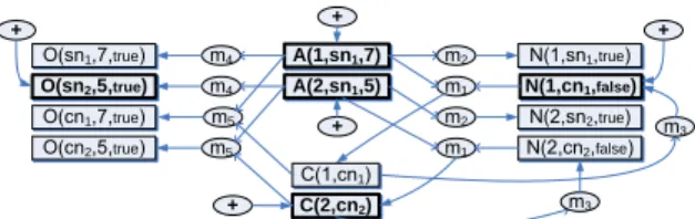
Figure 1: Example provenance graph (rectangles are tuples, ellipses are derivations, and ovals with ’+’ represent original base data, also shown as boldface).

are what we term theprovenanceof each tuple, and they can be described in terms ofbase data(EDBs), other derived tuples (for recursive derivations), and mappings (using the name that we have assigned to each rule). Moreover, a tuple may be the result of com-positionof mappings (which may also involve joins): e.g., a tuple may be derived in instanceOas a result of applyingm5to data in Cthat was mapped fromAandNalongm1. Our goal is to record

how data was derived through the mappings.

Figure 1 illustrates the result of data exchange over the mappings of Example 2.1 along with the relationship between tuples and their derivations. Thisprovenance graphhas two types of nodes: tuples (represented in rectangles, labeled with the values of the tuples) and derivations (represented as ellipses, labeled with the names of the mappings). This graph describes the relative derivations of tuples in terms of one another; local contribution tables for each relation contain the tuples indicated by boldface, and their presence is in-dicated by oval nodes with a ‘+’. Given a tuple node in the prove-nance graph, we can find itsalternate direct derivationsby finding the set of derivation nodes that have directed edges pointing to it. (These represent union.) In turn, each derivation has a set ofm source tuples that are joined — the set of tuple nodes with edges going to the derivation node — and a set ofnconsequents — the set of tuple nodes that have edges pointing to them from the deriva-tion node. The unique properties of our graph model will provide a desideratum for our provenance query language semantics: when-ever we return a derivation node in the output, we willalsowant all msource nodes andntarget nodes, to maintain the meaning of the derivation. This contrasts with the graph data models of [1, 16, 22, 32].

Use Cases for Provenance Graph Queries

Given this provenance graph, there are many scenarios where a user (especially through a graphical tool) may want to retrieve and browse a portion of the graph. Based on our discussions with scien-tific users, and on previous work in the data integration community, we consider several query use cases.

Q1. The ways a tuple was derived. A scientist, intelligence ana-lyst, or author of mappings [14] may want to visualize the different ways a tuple can be derived — including the source tuple values and the combination of mappings used. This is essentially a projection of the provenance graph, containing all base tuples from which the tuple of interest is derivable, as well as the derivations themselves, including the mappings involved and intermediate tuples that were produced. This graph may be visualized for the user.

Q2. Relationships between tuples. One may also be interested in restricting the set of derivations to those involving tuples from a certain source or derived relation or set of relations, e.g., if that relation is known to be authoritative [9].

Q3. Results derivable from a given mapping or view. The above use cases started with a tuple and considered its provenance. Conversely, we can query the provenance for tuples derived using a particular mapping (as is useful in [14]) or from a particular source.

Q4. Identifying tuples with common/overlapping provenance

As data is propagated along different paths in a CDSS, it may be useful to be able to determine at a given time whether tuples at two different peers have some common provenance. For instance, sup-pose we are trying to assess trustworthiness of information accord-ing to the number of peers in which it appearsindependently[20]. In that case, it is important to be able to identify when information came from the same peer or source.

2.1 From Provenance to Tuple Annotations

In the previous section and in our actual storage model, we focus on provenance as a graph. However, formally this graph encodes a (possibly recursively defined) set ofprovenance polynomialsin a provenance semiring[29] (also calledhow-provenance). This cor-respondence is useful in computingannotationslike scores, proba-bilities, counts, or derivability of tuples in a view.

Suppose we are given a provenance graph such as that of Fig-ure 1, and that every EDB tuple node is annotated with a base value: perhaps the Booleantruevalue if we are testing for deriv-ability, a real-valued tuple weight if we are performing approximate keyword search over the tuples, etc. Then we can compute anno-tations for the remaining nodes in abottom-up fashion: for any derivation node whose source tuple nodes have all been given an-notations, we combine the source tuple nodes’ annotation values with an appropriateabstract product operation: we AND Boolean values for derivability, or sum tuple weights in the keyword search model. When we reach a tuple node whose derivation nodes have all been given scores, we apply anabstract sum operationto deter-mine which annotation to apply to the tuple node: we OR Boolean values from the mappings for derivability, or compute the MIN an-notation of the different derivation nodes’ weights in the keyword search model. Finally, mappings themselves can affect the result-ing annotation, e.g., an untrusted mappresult-ing may producefalseon all inputs. We repeat the process until all nodes have been annotated.

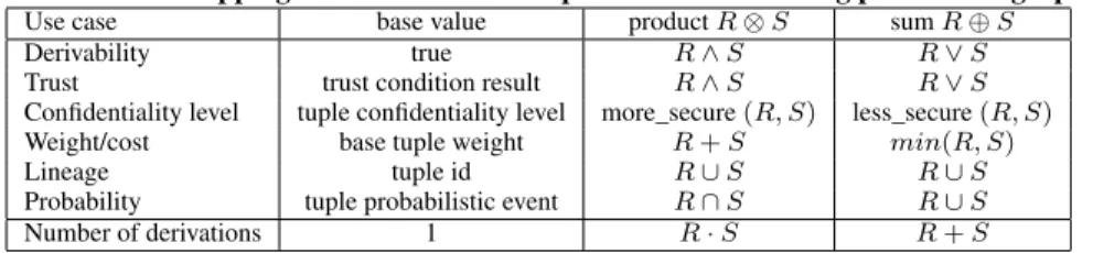
We can get different types of annotations for different use cases, based on how we instantiate thebase value,abstract product oper-ation, andabstract sum operation. The work of [29, 31] provides a formal definition of the properties that must hold for these values and operations, namely that they satisfy the constraints of a semir-ing; but we summarize some useful cases (including a few novel ones) in Table 1. Each row in the table represents a particular use case, and its semiring implementation.

Thederivabilitysemiring assignstrueto all base tuples, and de-termines whether a tuple (whose annotation must also betruecan be derived from them. Trustis very similar, except that we must check each EDB tuple to see whether it is trusted — annotating it withtrueorfalse. Moreover, each mapping may be associated with the neutral functionNm, returning its input value unchanged, or the distrust functionDm, returningfalseon all inputs. Any de-rived tuples with annotationtrueare trusted. Theconfidentiality levelsemiring [24] assigns a confidentiality access level to a tuple derived by joining multiple source tuples: for any join, it assigns the highest (most secure) level of any input tuple to the result; for any union, it assigns the lowest (least secure) level required. The

weight/costsemiring is useful in ranked models where output tu-ples are given a cost, evaluating to the sums of the individual scores or weights of atoms joined (and to the lowest cost of different al-ternatives in a union). This semiring can be used to produce ranked results in keyword search [41] or to assess data quality. The prob-abilitysemiring represents probabilistic event expressions that can be used for query answering in probabilistic databases.2 _The lin-2_{As observed in [19], computing actual probabilities from these}

(6)

Table 1: Useful mappings of base values and operations in evaluating provenance graphs.

Use case base value productR⊗S sumR⊕S

Derivability true R∧S R∨S

Trust trust condition result R∧S R∨S

Confidentiality level tuple confidentiality level more_secure(R, S) less_secure(R, S)

Weight/cost base tuple weight R+S min(R, S)

Lineage tuple id R∪S R∪S

Probability tuple probabilistic event R∩S R∪S

Number of derivations 1 R·S R+S

eagesemiring corresponds to the set of all base tuples contributing to some derivation of a tuple. Thenumber of derivations semir-ing counts the number of ways each tuple is derived, as in the bag relational model.

Cycles (recursive mappings). For provenance graphs contain-ing cycles (due to recursive mappcontain-ings) there are certain limitations. The first 5 semirings of Table 1 have idempotence and absorption properties guaranteeing they will remain finite in the presence of cycles (if evaluation is done in a particular way); for the number of derivations semiring, the annotations may not converge to a fi-nal value (i.e., we can have infinite counts). In this paper we de-velop a query language capable of handling cycles (as can occur in a CDSS such as ORCHESTRA, where participants independently specify schema mappings to their individual databases instances). However, we focus our initial implementation on the acyclic case.

Use Cases for Tuple Annotation Computation

Within data integration and exchange settings, there are a variety of cases where we would like to assign an annotation to each result in a materialized view, based on its provenance.

Q5. Whether a tuple remains derivable. During incremental view maintenance or update exchange, when a base tuple is de-rived, we need to determine whether existing view tuples remain derivable. Provenance can speed up this test [28].

Q6. Lineage of a tuple. During view update or bidirectional update exchange [33] it is possible to determine at run-time whether update propagation can be performed without side effects based on the derivability test ofQ5and thelineages[18] of tuples — i.e., the set of all base tuples each can be derived from, without distinguishing among different derivations.

Q7. Whether to trust a tuple. In CDSS settings, a set oftrust policiesis used to assign trust/distrust and authority levels to differ-ent data sources, views, and mappings — resulting in atrust level for each derived tuple based on its provenance [28, 42].

Q8. A tuple’s rank or score. In keyword query systems over databases, it is common to represent the data instance or the schema as a graph, where edges represent join paths (e.g., along foreign keys) between relations. These edges may have differentcosts depending on similarity, authority, data quality, etc. These costs may be assigned by the common TF/IDF document/phrase similar-ity metric, by ObjectRank and similar authorsimilar-ity-based schemes [4], or by machine learning based on user feedback about query an-swers [41]. The score of each tuple is a function of its provenance. If we are given a materialized view in this setting, we may wish to store the provenance, rather than the ranking, in the event that costs over the same edges might be assigned differently based on the user or the query context [41].

Q9. A tuple’s associated probability. In Trio [6], a form of provenance (called lineage in [6], though more general than that of [18]) is computed for query results, and then probabilities are from probabilistic databases [19] can be used to compute them more efficiently; this is outside the scope of this paper.

assigned based on this lineage. In similar fashion, we can compute probabilities from a materialized representation of provenance.

Q10. Computing confidentiality/access control levels for data.

Recent work [24] has shown how provenance can be used to assign access control levels to different tuples in a database. If the tuples might represent “shredded XML,” i.e., a relational representation of an XML document, then the access control level of a tuple (XML node) should be the strictest access control level of any node along the path from the XML root. In relational terms, the access control level of a tuple represents the strictest level of any tuple in a join expression corresponding to path evaluation.

In the next section, we describe a general language for express-ing a wide variety of provenance queries, includexpress-ing these use cases.

3. A QUERY LANGUAGE FOR PROVENANCE

To address the provenance querying needs of CDSS users, as ex-pressed in the use cases of the previous section, we propose a lan-guage, ProQL (forProvenanceQueryLanguage). We noted previ-ously that our use cases can be divided into ones that (1) help a user or application determine the relationship between sets of tuples, or between mappings and tuples; (2) provide ascore/rank,access con-trol levelorassessment of derivabilityortrustfor a tuple or set of tuples. Consequently, ProQL has two core constructs. The first de-finesprojections of the provenance graph, typically with respect to some tuple or tuples of interest. The second specifies how to evalu-ate a returned subgraph as an expression under a specific semiring, tocompute an annotationfrom that semiring for each tuple.

3.1 Core ProQL Semantics

A ProQL query takes as its input a provenance graphG, like the one of Figure 1. Thegraph projectionpart of the query:

• Matches parts of the input graph according topath expres-sions(possibly filtering them based on various predicates).

• Binds variables on tuple and derivation nodes of matched paths.

• Returns an output provenance graphG0, that is asubgraph ofGand is composed of the set of paths returned by the query. For each derivation node, every tuple node to which it is related is also returned inG0, maintaining the arity of the mapping.

• Returns tuples of bindings from distinguished query vari-ables to nodes inG0, henceforth calleddistinguished nodes. Note that provenance is a record of how data was related through mappings and data exchange; it does not make sense to be able to independently “create new provenance” within a provenance query language. Hence, unlike GraphLog [16], Lorel [1] or StruQL [22] — but similarly to XPath — ProQL cannot create new nodes or graphs, but always returns a subgraph of the original graph. More-over, provenance graphs are different from the graph models of those languages, in containing two kinds of nodes (tuple and deriva-tion nodes, where, as previously described, a derivaderiva-tion node is in some sense “inseparable” from the set of tuple nodes it relates).

(7)

If the ProQL query only consists of a graph projection part, it returns the subgraph described above, together with sets of bind-ings for the distinguished variables. The set of bindbind-ings accom-panying the graph projection is especially useful for the optional next stage: ProQL queries can also supportannotation computa-tionfor the nodes referenced in the binding tuples, using a par-ticular semiring. This is a unique feature of ProQL compared to other graph query languages, that is enabled by the fact that prove-nance graphs can be used to compute annotations in various semir-ings, as explained in Section 2.1. The annotation computation part of a ProQL query specifies an assignment of values from a par-ticular semiring (e.g., trust value, Boolean, score) to some of the nodes inG0and computes the values in that semiring for the dis-tinguished nodes. The result is a set of tuples consisting of pairs

(distinguished node id, semiring annotation value)for each bound variable output by the query.

Due to space limitations, this paper focuses on a single ProQL query block, but our design generalizes to support nested graph projection and annotation computation queries. For the latter, we need to retain both the annotations and the subgraph over which they were computed, in order to evaluate the outer query.

3.2 ProQL Syntax

As we explained above, ProQL queries can have two main com-ponents, graph projection and annotation computation. The graph projection part can be used independently, if one only needs to compute a projection of a provenance graph. The annotation com-putation part can apply an assignment to a provenance graph and compute values for its distinguished nodes in the corresponding semiring. To simplify the presentation, we explain the two core constructs of ProQL and their basic clauses, separately. An EBNF grammar for our language can be found in [31].

3.2.1 Graph Projection

Unlike the graphs typically considered in semi-structured data, our provenance graph is not rooted. We adopt a path expression syntax where the individual “steps” consist of traversals from a node representing a tuple in a relation, through a node represent-ing a derivation through a mapprepresent-ing, to another node representrepresent-ing a tuple. We refer to the actual nodes in the provenance graph astuple nodesandderivation nodes, respectively. Within the path expres-sion, we may restrict the tuple nodes to belong to a certain relation, or the derivation nodes to belong to a certain mapping. We may also bind variables to either type of node. We use the syntax:

[relation-name variable]

to indicate tuple nodes (where bothrelation-nameandvariableare optional), and one of the three forms:

<-|<mapping-name|<variable

to indicate derivation nodes (belonging to the corresponding map-ping). A schema mappingMin general may havemsource atoms andntarget atoms. Thus, in contrast to other graph models and query languages, even if a path expression includes one source and/or target atom, any matched derivation node corresponding to Mwill haventuple nodes to its left andmtuple nodes to its right. We also allow for arbitrary paths (compositions of multiple steps) between nodes, using the notation<-+for paths of length one or more. Paths may not be bound to variables.

Given this path notation, we outline our basic ProQL syntax, comprising 4 basic clauses (see [31] for further detail).

FOR: This clause binds variables (whose names are prefixed with the$character) to sets of tuple and/or derivation nodes in the graph, through path expressions.

WHERE: This clause is used to specify filtering conditions on the

variables bound in theFORclause. Conditions on tuple nodes may be expressed over the attributes of the tuple, or over the name of the relation in which it belongs. Derivation nodes may be tested for their mapping name. If path expressions are included in theWHERE

clause they are evaluated as existential conditions.

INCLUDE PATH: For each set of bound variables satisfying the

WHEREclause, this clause specifies the nodes and paths to be copied to the output graph. If a derivation node variable is output, its source and target tuple nodes are also output. At the end of query execution, the output graph unifies all nodes and paths that have been copied throughINCLUDE PATHoperations.

RETURN: In addition to returning a graph, it is essential that we be able to identify specific nodes in this graph. TheRETURNclause specifies the set of distinguished variables whose bindings are to be returned together as result tuples.

Using these clauses, we can express ProQL queries for the first four use cases of Section 1.

Q1. Given the setting of Figure 1, return the subgraph containing all derivations of tuples inOfrom base tuples:

FOR [O $x]

INCLUDE PATH [$x] <-+ [] RETURN $x

Note the use of the path wildcard (<-+) specifying all paths from all nodes that derive any$xnode.

Q2. Return the part of derivations of tuples inOthat involve tuples in relationA.

FOR [O $x] <-+ [A $y] INCLUDE PATH [$x] <-+ [$y] RETURN $x

Q3. Find tuples that can be derived through mappingsm1orm2 and return all one-step derivations from those tuples.

FOR [$x] <$p [], [$y] <- [$x] WHERE $p = m1 OR $p = m2

INCLUDE PATH [$y] <- [$x] RETURN $y

Note the comparison as to whether$pis from mappingsm1orm2. Reusing$xin the second path expression is a syntactic shortcut im-plying a join between paths matched by the two path expressions.

Q4. Select tuples fromOandCthat have common provenance (called “join using provenance” in [13]), and return their deriva-tions:

FOR [O $x] <-+ [$z], [C $y] <-+ [$z] INCLUDE PATH [$x] <-+ [], [$y] <-+ [] RETURN $x, $y

Observe that there are two variables in theRETURNclause of the query above. As a result, this query returns pairs of bindings to tuple nodes in the provenance graph that have common provenance.

3.2.2 Annotation Computation

We now consider how to take returned subgraphs and use them to compute semiring annotations for sets of tuples — matching the needs of our remaining use cases. For this situation, we add two new clauses to ProQL.

EVALUATEsemiringOF: This clause is used to specify the semir-ing for which we want to evaluate the graph returned by the nested graph projection query. Semirings built into our implementation include those presented in Table 1, and we expect that future imple-menters of ProQL may wish to add additional semirings to match their domain requirements.

ASSIGNING EACH: To compute annotations in particular semir-ings, one needs to assign values from that semiring toleaf nodes, i.e., EDB tuple nodes in the original graph or tuple nodes that have no incoming derivations in projected subgraphs; as well as to define appropriate unary functions for the mappings. TheASSIGNING EACHclause can be used to specify such assignments similarly to a switchstatement in C or Java: first, we define a variable that iterates over the set of leaf nodes from the query’s projected provenance

(8)

subgraph, and then we list cases and the value to assign a node, should the case be met.3 _{In these conditions one can check}

mem-bership in a relation or express selections on values of particular attributes of the corresponding tuples. Finally, there is an optional

DEFAULTstatement, if none of theCASEstatements is satisfied. If there is noDEFAULTstatement, all leaf nodes not matching any

CASEare assigned the identity element for the·operation of the semiring.

Similarly, a secondASSIGNING EACHclause can be used to define unary mapping functions in each semiring. In this case, one can specify conditions over the name of a mapping as well as the semiring value of its single parameter. The default value for map-pings, if noDEFAULTstatement is provided, is the identity func-tion. Function definitions are restricted in two key ways [31]: one cannot specify an assignment that returns a non-zero value when the input is0and mapping application must commute with (finite and infinite) sums.

Any (or both) of these two kinds ofASSIGNING EACHclauses may be specified in a query, depending on whether a user wants to “customize” their value assignment for leaf nodes and/or mappings or they are satisfied with default values. We illustrate the usage of theASSIGNING EACHclause(s) in the following queries for use casesQ5-Q10of Section 1.

Q5. Determine derivability of the tuples inU from base tuples (the default assignment is sufficient in this case).

EVALUATE DERIVABILITY OF{ FOR [O $x]

}

Q6. Same as above, but substitute the word “LINEAGE” for “DERIVABILITY”.

Q7. Assuming peerOdistrusts any tupleO(n, h, a)if the data came fromA(i, n, h)andh≥6, trusts any tuple fromCand dis-trustsm4while trusting all other mappings if their input is trusted, determine what set of tuples inOis trusted:

EVALUATE TRUST OF{ FOR [O $x]

} ASSIGNING EACH leaf_node $y { CASE $y in C : SET true

CASE $y in A and $y.height >= 6 : SET false DEFAULT : SET true

} ASSIGNING EACH mapping $p($z) { CASE $p = m4 : SET false DEFAULT : SET $z }

Q8-Q10. These are similar toQ7, using the “WEIGHT”, “PROB

-ABILITY” and “CONFIDENTIALITY” semirings, respectively, and assigning appropriate base values for each semiring.

4. STORING & PROCESSING PROVENANCE

In this section we describe our prototype implementation of the core operations of the language, as presented earlier. Our imple-mentation is built on top of the standalone ORCHESTRAengine [28], that creates a complete replica of all data and provenance in the CDSS at each peer, to accomodate disagreements among peers, and uses each peer’s relational DBMS for provenance storage and querying. To this end, we describe the core aspects of our prove-nance encoding in relations, and our query execution strategy that exploits a relational DBMS engine. The next section discusses how we enhance this basic engine with indexing techniques.

4.1 Provenance Storage in Relations

Extending the ORCHESTRA implementation of [28], we store provenance in a set of relations in an RDBMS. Intuitively, we would

3

if multipleCASEstatements match, the first one is followed

P2(i, n, true):-A(i, n, l) P4(n, h, true):-A(i, n, h) P3(i, n, f alse):-C(i, n) P1(i, n) 1 cn1 2 cn2 P5(i, n) 1 cn1 2 cn2

Figure 2: Relations corresponding to Figure 1, assuming the key of Ais id, that of C andN is the pair (id, name) and the key ofOisname. Provenance relationsP2, P3, P4are

su-perfluous because the mappings are projections overAandC, hence they are replaced with views.

like a scheme resembling theedge relationencoding of a tree or graph (i.e., a relation in which tuples contain source and destina-tion attributes). Of course, mappings in our setting are not strictly binary relationships — we can map frommsource tuples ton tar-get tuples. We observe that each relation connected by provenance can be identified by its key. Hence we encode a single mapping derivation in a relation containing the keys of allmsource andn target relations. For compactness, we only store one copy of any set of attributes that are constrained by the mapping to be the same (e.g., attributes joined on equality, or copied from input to output relations). Each tuple in the provenance relation exactly represents a derivation node and its outgoing edges, as in Figure 1. Each tuple node is simply a tuple in one of the database relations. Our scheme differs from that of [28], in that each derivation is represented by a single tuple: in that work, there were certain cases (specifically with Skolem functions) where that was not the case.

Superfluous Provenance Relations. If we refer back to Example 2.1, we see that mappingm2computesN by projecting over the attributes ofA, and adding a constanttrue. Herem2’s provenance relation would contain the key attributes ofA, and we can add the remaining (constant) attribute forN simply by knowing the def-inition ofm2. Hence we consider this provenance relation to be superfluous: rather than materializing a table form2, we define it as a virtual view overA.

Combining Provenance Relations. Unfortunately, a general problem that arises using a relational encoding is that there are many potential path traversals through different combinations of provenance relations; and the result is a large number of queries (for alternate paths) with multiple joins (representing multiple nodes on a path). A natural question is how best tocombineprovenance re-lations to improve performance. In [28], we established that it was more effective to take all source and target tuples’ key attributes for a single schema mapping and store these in their own provenance table — as opposed to storing data from multiple derivations with the same target relation in a combined table that used disjoint union. Hence we build upon this idea, and we show in Section 5 how we can index combinations of such provenance tables to optimize path traversals.

EXAMPLE 4.1. For our running example of Figure 1, suppose that the key ofAisid, that ofCandNis the pair(id, name)and the key ofOisname. Figure 2 shows the provenance relations (wherePicorresponds to mappingmi).

4.2 Translating ProQL to SQL

In this section, we describe our strategy for executing ProQL queries that return projections of the provenance graph or compute annotations based on a provenance graph. ProQL queries may in-clude conditions in theWHEREclause specifying aset of tuplesof interest. For instance, perhaps we have a screenful of tuples from

(9)

A N m5 O m2 C m1 m3 m4

Figure 3: Provenance schema graph for running example

some relationRfor which we wish to compute rankings. Rather than compute a ProQL query overalltuples inR, we would like to performgoal-directedcomputation such that we only evaluate provenance for the selected tuples, as well as only for the paths matching the path expressions in the query. Intuitively, this resem-bles pushing selections through joins in relational algebra queries.

We assume that provenance graphs are stored in an RDBMS, according to our relational encoding of the previous section. Thus, our approach relies on converting ProQL queries into SQL queries (or, generally, sets of SQL queries) that can ultimately be executed over an underlying RDBMS. More precisely, we break the query answering process into several stages:

• Convert the schema mappings into aprovenance schema graph (this is common for all queries).

• Match the ProQL query against the provenance schema graph to identify nodes that match path expressions.

• Create a Datalog program based on the set of schema map-pings and provenance relations that correspond to the schema graph nodes, as well as the source relations whose EDB data is to be included.

• Execute the program in an SQL DBMS, in a goal-directed fashion, based on tuples and mappings of interest.

We explain each of these stages in more detail below.

4.2.1 Provenance Schema Graph

While paths in the provenance graph exist at the instance (tu-ple) level, in fact these tuples belong to specific relations that are connected through mappings defined at the schema level. Hence, it makes sense to abstract the set of possible provenance relationships among tuples into a set of potential derivations among relations — in essence to define a schema for the provenance. Intuitively simi-lar to a Dataguide [27] over the provenance, this graph is useful as a basis for matching patterns and ultimately defining queries.

We term this graph among relations and mappings aprovenance schema graph, constructed as follows. First, we create one node for each relation (arelation node, labeled with the name of the relation) and onemapping nodefor each mapping (labeled with the mapping name). Then, we add directed edges from the mapping node to a relation node if the mapping has a target atom matching the relation node’s label. Finally, we add directed edges from a relation node to the mapping node if the mapping has a source atom matching the relation node’s label. The result looks like Figure 3, where we show relation nodes with rectangles and mapping nodes with ellipses.

4.2.2 Matching ProQL Patterns

The next step is to determine which subgraphs of the provenance schema graph match the ProQL patterns. We start with the dis-tinguished reference nodes of the ProQL query: these nodes can range over all relations or may be restricted to a single relation, if specified by the query. For each path expression in theFORclause, our algorithm traverses the schema graph from each node that can match the “originating” node of the path, using a nondeterministic-state-machine-based scheme to find paths that match the pattern. (We prevent paths from cycling back upon themselves.) The ulti-mate result is a set of mapping nodes and relation nodes.

4.2.3 Creating a Datalog Program

As an intermediate step towards creating the ultimate SQL queries to return answers, we first create a Datalog program based on the set of mapping and relation nodes returned by the pattern-match.4_This

process is fairly straightforward. For each mapping node returned from the matching step, we add the corresponding mapping to the program. For every relation node matched in the schema graph, we also add rules to test if we have reached a local contribution relation (containing leaf nodes of the provenance graph).

EXAMPLE 4.2. For our running example, suppose we want to evaluate a query returning all derivations of tuples inOfrom tu-ples inAandN. From the provenance schema graph of Figure 3 the matching step will returnm4, which definesOin terms ofA,

as well asm1, which derives tuples inCfromAandN, which can

then be combined withAthroughm5, to derive tuples inO. Then,

the Datalog program contains rules for these mappings involving the corresponding provenance relations; e.g., form5this rule is:

O(n, h, true):-P5(i, n), A(i,_, h), C(i, n)

Moreover, the Datalog program contains rulesL1, L3, L4from

Ex-ample 2.1, in order to test whether tuples of interest may be derived from the local contributions of one of the matched relations.

In order to represent the returned graph of a ProQL query we create a set of output tables — one for each relevant provenance relation — and populate them with the edges in the output sub-graph. Queries also return a relational result containing the tuple keys (possibly paired with an annotation from some semiring) for the bindings in theRETURNclause.

4.2.4 Executing the Program

We now consider how to execute the Datalog version of our ProQL query over a provenance graph stored in an RDBMS. Re-call the contents of the provenance relations for our running exam-ple, as shown in Figure 2. In order to reconstruct partial or com-plete derivations of a tuple — as described in path expressions in the graph projection part of ProQL queries — we need to com-bine tuples from multiple provenance relations. Moreover, to exe-cute ProQL queries with an annotation computation component, we need to identify complete derivations from leaf nodes, for which an assignment of semiring values is given in the query.

For acyclic provenance graphs, each tuple can only have a finite number ofdistinct derivation tree shapes. For each of those deriva-tion shapes, we can compute a conjunctive rule that reconstructs them from the one-step derivations stored in the provenance rela-tions, byrecursively unfoldingthe rules of the Datalog program of Section 4.2.3. The result is a union of conjunctive rules over prove-nance relations and base data “reachable” from them.

EXAMPLE 4.3. Continuing our running example, in the body of the rule shown in Example 4.2, tuples inAcan only be derived locally (fromAl) while tuples inCcan be derived either fromCl or throughm1(m3does not match since the query only asked for

derivations from tuples inAandN). Then, one (breadth-first) un-folding step yields the rules:

O(n, h, true):-P5(i, n), Al(i,_, h), Cl(i, n)

O(n, h, true):-P5(i, n), Al(i,_, h), P1(i, n), A(i, s,_), N(i, n, f alse)

We repeat this process (using only rules matching the ProQL pat-tern) until all body atoms in all rules are either provenance relation atoms or local contribution relation atoms.

During this unfolding we can create a semiring expression cor-responding to this derivation tree shape. This expression can then

4

This program can be recursive for cyclic provenance graphs. However, in this paper we focused on ProQL evaluation over acyclic provenance graphs, for which this program is not recursive.

(10)

be used to compute annotations, by “plugging in” annotations for leaf nodes and combining them with the appropriate semiring mul-tiplication operation at intermediate tree nodes.

Of course, each conjunctive rule only computes a subset of the tuples and their provenance — specifically the tuples and prove-nance values for one potential derivation tree. We convert each conjunctive rule into SQL (adding an additional attribute for the provenance expression evaluation). Then, we take the resulting SQL SELECT..FROM..WHERE blocks and combine their output using SQL UNION ALL. Finally, we evaluate an aggregation query over the combined output, in which we GROUP BY the values of the tuples, then combine the provenance attributes using an aggre-gation function, and finally threshold the results with a HAVING expression. Referring to Table 1, for the first two semirings (deriv-ability and trust), we can SUM the annotations (assuming we repre-senttrueas 1 andfalseas 0), then add a HAVING clause testing for a non-zero annotations. The next two expressions can be evaluated using MIN; and the number of derivations can be SUMmed.

These components form a baseline implementation of ProQL, providing all the required functionality. However, more can be done to improve its performance. In the next section we intro-duce indexing techniques that can be used to speed up processing of provenance queries.

5. INDEXING DATA PROVENANCE

The main challenge in answering ProQL queries lies in navigat-ing through graph-structured data, accordnavigat-ing to unrooted path ex-pressions. As we explained in Section 4.2, such path traversals are translated into joins among provenance relations, each representing a one-step derivation. Such paths in provenance graphs can often be long, and their translation produces unfolded rules containing multi-way joins, whose execution can be expensive. Moreover, dif-ferent unfolded rules may contain overlapping paths, meaning that multiple rules may contain common join subexpressions.

A natural question to ask is whether one could optimize ProQL queries by precomputing the shared joins, i.e.,indexingpaths in a provenance graph. Then, queries involving those paths can start at one node and find sets of nodes reachable within a certain number of hops directly from this index, without needing to join individ-ual provenance relations. Ideally, such an index structure could be retrofitted into a relational DBMS engine, so that our SQL-based strategy could benefit from it.

Among a variety of path indices that have been studied in the literature [17, 27, 35, 37], the most natural indexing technique to adapt for our provenance query scheme is theaccess support rela-tion[35] (ASR) originally developed for object-oriented databases. An ASR is ann-ary relation among sets of objects connected through paths that can be used to speed up queries involving path expres-sions in object-oriented query languages. Unlike the other types of path indices, ASRs can be emulated using conventional rela-tional tables, which reference the base tables on (B-Tree) indexed attributes. This provides very similar performance to having built-in support for ASR structures, while havbuilt-ing the virtue that it will run on any off-the-shelf RDBMS.

In the case of object-oriented databases, each object has a unique object identifier (OID) and the ASR is an auxiliary structure known to the DBMS, consisting of tuples with references to objects by their OIDs. Clearly, in our case we neither have objects nor OIDs. Moreover, our patterns have some subtle differences from paths in the object-oriented sense. However, one can take most of the basic principles of the ASR and extend them to match our setting.

In particular, we can define ASRs for paths in provenance graphs by creatingmaterialized viewsfor joins among provenance

rela-tions that correspond to paths of mappings along some derivarela-tions. These views can also be stored as relations in the RDBMS, to-gether with the provenance relations. Then, rewriting unfolded rules to take advantage of such ASRs amounts to a case of answer-ing queries usanswer-ing materialized views [30]. Moreover, we can define relational indices on key columns of the ASRs to provide efficient lookup of specific rows (corresponding to paths in particular deriva-tions) as well as to optimize queries that involve longer paths (and, therefore, need to join multiple ASRs).

In the rest of this section we explore different options regarding how to adapt ASRs so that they can be combined with our relational storage of provenance to speed up processing of ProQL queries. These options also determine the appropriate schema for the rela-tional storage of the resulting ASRs.

5.1 ASR Design Choices

To index paths in a provenance graph, we need to materialize the results of joins among provenance relations: each relation repre-sents an edge traversal, and an index reprerepre-sents a traversal of mul-tiple edges. However, as we index a path within an ASR, we have several choices about whether to also index some or all of its sub-paths. In this section, we discuss these options and their likely ad-vantages and disadad-vantages. Later we discuss their implementation and experimentally compare them.

The choice of whether to materialize only the complete path or (some or all of) its subpaths impacts how we join the provenance relations in forming the ASR. In particular, for a two-step ASR, an inner join among provenance relations represents a complete path, a left outerjoin results in a path and its prefixes (padded by NULLs in the resulting ASR), a right outerjoin represents a path and its suffixes, and a full outerjoin represents a path and all its subpaths.

To include paths and subpaths within a longer (e.g., 3-step) ASR, we may need to union together the results of multiple queries. Sup-pose we have a path through provenance tablesP3←P2←P1. Naively outerjoining multiple steps, e.g., some set of linked prove-nance tablesP3−−1−−P2−−1−−P1, might result in ASR tuples con-taining entries fromP3andP1, with NULLs in place ofP2(since there might not exist an edge connecting these steps). Instead, we can index all subpaths in this case by unioning a pair of joins:

P(3,2,1)=P31P2−−1−−P1∪P3−−1−−P21P1 In the rest of this paper, we use the termssubpath ASR,prefix ASRand suffix ASRto refer to ASRs based on these operations, which index a path as well as all its subpaths, prefixes or suffixes, respectively, andcomplete path ASRfor the ASR that only con-tains the inner join of all mappings. We note that inner joins can be expressed as Datalog rules and thus can easily be maintained incrementally, together with regular provenance relations [28]. In-cremental maintenance of outerjoins is more complicated and we intend to explore it in future work.

5.2 Using ASRs in ProQL Query Evaluation

In order to take advantage of ASRs, we need to rewrite the rules in the Datalog program of Section 4.2.4 — replacing provenance relation atoms with ASRs that contain those provenance relations. In essence, this is a matter of substituting materialized views, which we cannot always depend on from an underlying RDBMS.

One factor that can significantly complicate this rewriting pro-cess is the existence of overlapping ASR definitions, i.e., when dif-ferent ASRs may index overlapping (sub)paths. Here, in order to produce a minimal rewriting (i.e., one with the smallest possible number of atoms) we would need to follow an expensive dynamic programming approach, considering the ASRs in all possible or-ders. We note that this rewriting needs to be performed at execution

(11)

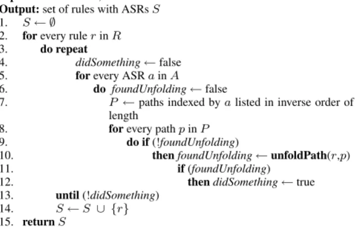
Algorithm unfoldASRs

Input:set of rulesR, set of ASRsA

Output:set of rules with ASRsS

1. S← ∅

2. forevery rulerinR

3. do repeat

4. didSomething←false

5. forevery ASRainA

6. do foundUnfolding←false

7. P ←paths indexed byalisted in inverse order of length

8. forevery pathpinP

9. do if(!foundUnfolding)

10. thenfoundUnfolding←unfoldPath(r,p) 11. if(foundUnfolding)

12. thendidSomething←true

13. until(!didSomething)

14. S←S ∪ {r}

15. returnS

Algorithm unfoldPath

Input:ruler(modified if unfolding is found), rulep(representing a path in an ASR)

Output:true if unfolding was found, false otherwise

1. h←findHomomorphism(r,p)

2. if(h6= ∅)

3. then foreach variablexin the head and body ofp

4. doreplacexwithh(x) 5. foreach atomain the body ofp

6. doremoveafrom the body ofr

7. add the head ofpto the body ofr

8. returntrue

9. else

10. returnfalse

Algorithm findHomomorphism Input:ruler, rulep

Output:a homomorphism fromrtop(i.e., set of mappings from variables

inpto variables and constants inr) or∅, if no homomorphism exists 1. elided for brevity

Figure 4: ASR Rewriting Algorithm

time for each ProQL query, so being able to perform it efficiently is crucial for overall query performance.

For this reason, we chose to allow only non-overlapping ASR definitions, for which a minimal unfolding can always be produced by the greedy algorithmunfoldASRsof Figure 4. This algorithm considers each path contained in an ASR in inverse order of length. If there are no overlapping ASRs, this guarantees that the resulting unfolding is minimal, since (shorter) subpaths are only unfolded if it was impossible to unfold any of their (longer) superpaths.

In step 10,unfoldASRsemploys algorithmunfoldPath, which first looks for ahomomorphismfrom the body of the pathpto that of the ruler, i.e., a mapping from variables inpto variables and constants inrsuch that each atom in the body ofpis mapped to an atom in the body ofr. If such a homomorphism is found, it replaces those mapped atoms in the body ofrwith the image of the head of p(i.e., an ASR atom “selecting” the part of the ASR representing this subpath) under the homomorphism (replacing variables with the values to which they are mapped).

EXAMPLE 5.1. In our running example, if we define an ASR P(5,1)for the path ofm1followed bym5, the unfolding algorithm

would replace theP5andP1 atoms in the second rule of

Exam-ple 4.3 with aP(5,1)atom, producing the following rule which

con-tains one join fewer than the original one:

O(n, h, true):-P5,1(i, n), Al(i,_, h), A(i, s,_), N(i, n, f alse)

6. EXPERIMENTAL EVALUATION

Given the lack of established provenance query systems and bench-marks, we developed microbenchmarks for provenance queries. We

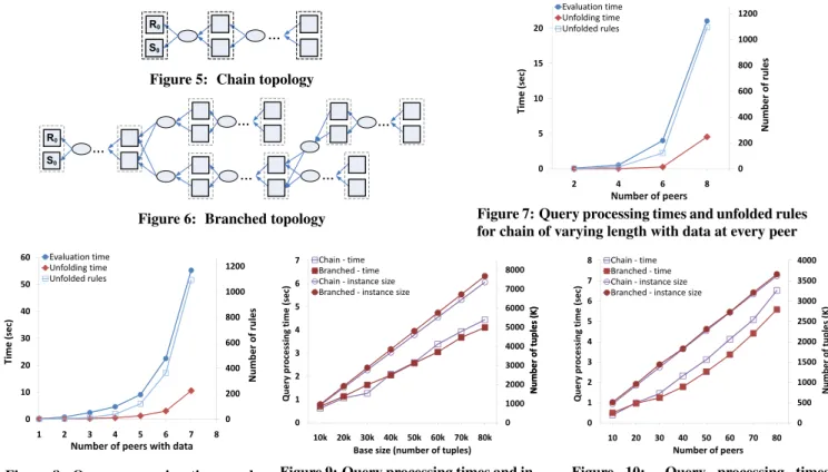
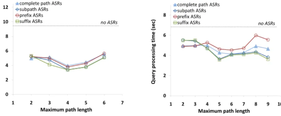
investigate the performance of path traversal queries, which are at the core of any provenance query, and the optimization benefits of ASRs for such queries on CDSS settings with different mapping topologies. First, we consider a simple topology, where all peers are connected through mappings that form achain, as shown in the provenance schema graph of Figure 5, in order to focus on specific factors that affect performance of provenance querying and illus-trate ASR optimization opportunities. Next, we experiment with a more realisticbranchedtopology, as shown in Figure 6, and in-vestigate the performance and scalability of provenance query pro-cessing, for different numbers of peers and amounts of data at each peer. Finally, we consider grouping mappings along paths in ASRs and analyze the performance benefits of ASRs of different types and lengths.

6.1 Experimental Setup

Our ProQL prototype, including parsing, unfolding and transla-tion to SQL queries was implemented as a Java layer running atop a relational DBMS engine. We used Java 6 (JDK 1.6.0_07) and Win-dows Server 2008 on a Xeon ES5440-based server with 8GB RAM. Our underlying DBMS was DB2 UDB 9.5 with 8GB of RAM.

6.1.1 Settings and Terminology

Due to the lack of real-world data sharing settings that are suf-ficiently large and complex to test our system at scale, we cre-ated synthetic workloads based on bioinformatics schemas and data from the SWISS-PROT protein database [3]. We generate peer schemas and mappings by partitioning the 25 attributes in the SWISS-PROT universal relation into two relations and adding a shared key to preserve losslessness. Then, each mapping has a join between two such relations in the body and another join between two rela-tions in the head.

In typical bioinformatics CDSS settings, one would expect most of the data to be contributed by a small subset of authoritative peers; thus, in most of our experiments we consider settings with rela-tively few peers with local data, while the remaining peers import data along incoming mappings, edit them according to their trust policies, and propagate them further along outgoing mappings. In our first experiment we also explore the scalability of provenance querying in a setting with local data at all peers, as a stress test.

Both of the topologies we experimented on have atargetpeer, which is the one that all mappings are propagating data to, directly or indirectly. This does not imply that we expect real-world settings to form rooted trees. In fact, these topologies should not be inter-preted as a complete CDSS setting, but rather as a projection of the complete mapping graph that only contains peers from which our target peer of interest is reachable. However, this projection allows us to focus on the extreme case, where all peers and mappings prop-agate data to this particular target peer. Typically, in a CDSS, there will be many peers and mappings that do not propagate data to this peer (e.g., other peers that import data from common authoritative sources) but those mapping paths do not affect the evaluation or the result of the provenance queries whose performance we measure.

We generate local data for each peer by sampling from the SWISS-PROT database and generating a new key by which the partitions may be rejoined. For these experiments, we substituted integer hash values for each large string in the SWISS-PROT database, model-ing the amount overhead taken by CLOBs in a real bioinformatics database. We refer to thebase sizeof a workload to mean the num-ber of SWISS-PROT entries inserted locally at each peer and prop-agated to the other peers before provenance queries were executed.

6.1.2 Provenance Queries

The main goal of these experiments is to evaluate the perfor-mance of the path traversal component of ProQL, with or without

(12)

Figure 5: Chain topology

0

Figure 6: Branched topology

600 800 1000 1200 10 15 20 m e (sec) Evaluation time Unfolding time Unfolded rules ro f rules 0 200 400 0 5 10 2 4 6 8 Ti m Number of peers Numbe Number of peers

Figure 7: Query processing times and unfolded rules for chain of varying length with data at every peer

600 800 1000 1200 30 40 50 60 m e (sec) Evaluation time Unfolding time Unfolded rules ro f rules 0 200 400 0 10 20 1 2 3 4 5 6 7 8 Ti m

Number of peers with data

Numbe

Number of peers with data

Figure 8: Query processing times and unfolded rules for chain of 20 peers with varying number of peers with data

4000 5000 6000 7000 8000 4 5 6 7 ssing time (sec) Chain ‐time Branched ‐time Chain ‐instance size Branched ‐instance size

f tuples (K) f tuples (K) 0 1000 2000 3000 4000 0 1 2 3 10k 20k 30k 40k 50k 60k 70k 80k Query pr oce s Number o f Number o f

Base size (number of tuples)

Figure 9: Query processing times and in-stance size for chain and branch topolo-gies of 20 peers and varying base sizes

2000 2500 3000 3500 4000 4 5 6 7 8 ssing time (sec) Chain ‐time Branched ‐time Chain ‐instance size Branched ‐instance size

f tuples (K) 0 500 1000 1500 0 1 2 3 10 20 30 40 50 60 70 80 Query pr oce s Number o f Number of peers

Figure 10: Query processing times and instance size for chain and branch topologies of varying numbers of peers

the use of ASRs. As a result, for our experiments, we used queries of the form (hereby calledtargetquery):

FOR [R0 $x]

whereR0is a relation at the target peer of the corresponding topol-ogy. Such queries traverse all the paths in the mapping graphs up to their end, and thus are ideal in order to evaluate path traversal.

We also experimented with similar queries involving annotation computation similar toQ7from Section 3.2. Perhaps surprisingly, we found that the execution time for queries involving such annota-tion computaannota-tions was very similar to that of their graph projecannota-tion component, i.e., the graph projection component dominates execu-tion time. Thus, for simplicity, in the experiments below we focus on graph projection queries without annotation computation.

6.1.3 Experimental Methodology

Each experiment was repeated seven times, with the best and worst results discarded, and the remaining five numbers averaged. In all of our experiments, the results were very similar among these five runs, and thus the confidence intervals were too small to be visible on the graphs.

6.2 Number of Peers with Local (Base) Tables

In the experiments of this section we use the chain topology of Figure 5. For the first experiment, we perform a “stress-test” by assuming that all peers have local data and investigate the perfor-mance of the target query shown above. Figure 7 shows that, in this case, the number of unfolded rules grows exponentially with the number of peers. Intuitively, this is because every tuple at ev-ery peer may either be inserted locally or derived from some peer further “downstream” in the graph of mappings, and the unfolding needs to cover all these possible derivations. Moreover, for every join we need to consider all combinations for each side of the join. Thus, as also shown in Figure 7, unfolding time and evaluation time

for the unfolded rules also grow exponentially, remaining efficient (sub-20 sec.) for up to 8 peers.

To isolate the effect of the number peers withlocal datawe re-peated this experiment for a fixed total number of peers, varying the number of local contribution relations. Figure 8 shows that the number of unfolded rules, as well as unfolding and evaluation times, also grow exponentially with the number of peers supplying local data, for a setting with 20 total peers.

6.3 Number of Peers and Base Size

As we explained earlier, in real-world bioinformatics settings it is more likely that only a small number of authoritative sources will contribute local data, that is then propagated along (possibly long) paths of mappings. For this reason, in the next experiments, we consider CDSS settings that have data at a few of the peers near the right-hand side of the topologies of Figures 5 and 6. Figure 9 shows that the size of the instances produced as a result of the prop-agation of local data at the grows linearly with the base size. Query processing time (i.e., the sum of unfolding and evaluation times) also grows linearly up to a few seconds, even for a base size of 80k tuples per peer relation.

In Figure 10 we show that the size of the instance that results from the propagation of 10k tuples inserted locally at a few (2-3) of the peers grows linearly with the total number of peers through which they are propagated. Query processing time also grows at a roughly linear rate for both topologies, although a bit faster for the branched topology. Moreover, it is within a few seconds, even for topologies of 80 peers. This implies that our implementation could scale to at least a few hundreds of peers, but we were unable to run experiments for settings with more than 80 peers because the resulting SQL queries were too large for DB2 (as each unfolded rule can contain up ton-way joins, wherenis roughly equal to the number of nodes in a derivation tree of the target peer).