TCP FTAT (Fast Transmit Adaptive Transmission): a New End-To-End Congestion Control Algorithm

(1)

Cleveland State University

EngagedScholarship@CSU

ETD Archive

2014

TCP FTAT (Fast Transmit Adaptive

Transmission): a New End-To-End Congestion

Control Algorithm

Mohammed Ahmed Melegy Mohammed Afifi

Cleveland State University

Follow this and additional works at:https://engagedscholarship.csuohio.edu/etdarchive Part of theElectrical and Computer Engineering Commons

How does access to this work benefit you? Let us know!

This Thesis is brought to you for free and open access by EngagedScholarship@CSU. It has been accepted for inclusion in ETD Archive by an authorized administrator of EngagedScholarship@CSU. For more information, please contactlibrary.es@csuohio.edu.

Recommended Citation

Afifi, Mohammed Ahmed Melegy Mohammed, "TCP FTAT (Fast Transmit Adaptive Transmission): a New End-To-End Congestion Control Algorithm" (2014).ETD Archive. 730.

(2)

TCP FTAT (Fast Transmit Adaptive Transmission): A NEW END-TO-

END CONGESTION CONTROL ALGORITHM

MOHAMMED AHMED MELEGY MOHAMMED AFIFI

Bachelor of Electronics Engineering and Technology World College

July 2011

submitted in partial fulfillment of requirements for the degree

MASTER OF SCIENCE IN ELECTRICAL ENGINEERING

at the

CLEVELAND STATE UNIVERSITY

December 2014

(3)

We hereby approve this thesis For

MOHAMMED AHMED MELEGY MOHAMMED AFIFI Candidate for the Master of Science in Electrical Engineering degree

For the Department of

Electrical and Computer Engineering And

CLEVELAND STATE UNIVERSITY’S College of Graduate Studies by

Dr. Nigamanth Sridhar, Committee Chair

Department & Date

Dr. Chansu Yu, Committee Member

Dr. Pong Chu, Committee Member

May 7, 2014

(4)

(5)

ACKNOWLEDGEMENTS

I would like to thank all those who gave me the opportunity to complete my thesis work. I would like to thank my advisor, Professor Nigamanth Sridhar, for all the

guidance and the support throughout my thesis work. I would also like to thank the Department of Electrical and Computer Engineering, of which I have had the pleasure being a student for the past two years.

(6)

TCP FTAT (Fast Transmit Adaptive Transmission): A NEW END-TO-

END CONGESTION CONTROL ALGORITHM

MOHAMMED AHMED MELEGY MOHAMMED AFIFI

ABSTRACT

Congestion Control in TCP is the algorithm that controls allocation of network resources for a number of competing users sharing a network. The nature of computer networks, which can be described from the TCP protocol perspective as unknown resources for unknown traffic of users, means that the functionality of the congestion control algorithm in TCP requires explicit feedback from the network on which it operates. Unfortunately this is not the way it works with TCP, as one of the fundamental principles of the TCP protocol is to be end-to-end, in order to be able to operate on any network, which can consist of hundreds of routers and hundreds of links with varying bandwidth and capacities. This fact requires the Congestion Control algorithm to be adaptive by nature, to adapt to the network environment under any given circumstances and to obtain the required feedback implicitly through observation and measurements. In this thesis we propose a new TCP end-to-end congestion control algorithm that provides performance improvements over existing TCP congestion control algorithms in computer networks in general, and an even greater improvement in wireless and/or high bandwidth- delay product networks.

(7)

vi

List of Figures

Figure 1: FSM Description of TCP Congestion Control [reproduced from 16]. ... 12

Figure 2: FSM description of Westwood [produced from 18, 19] ... 18

Figure 3: Black Box Principle in the Presence of Congestion ... 21

Figure 4: Black Box Principle in the Presence of Random Loss ... 22

Figure 5: Black Box Principle in the Presence of Congestion and Random Loss ... 23

Figure 6: Adaptive Transmission Effect ... 25

Figure 7: NewReno Congestion Window Pattern ... 27

Figure 8: FSM description of FTAT ... 30

Figure 9: TCP Implementation in ns-3 including FTAT... 34

Figure 10: Classes interaction in Linux ... 40

Figure 11: TCP function interaction in Linux ... 42

Figure 12: First Topology ... 49

Figure 13: cwnd graphs for Topology one ... 50

Figure 14: RTT graphs for topology two ... 52

Figure 15: Sequence number topology one ... 53

Figure 16: Throughput and Goodput topology one ... 55

Figure 17: Topology two ... 56

Figure 18: cwnd graphs topology two ... 57

Figure 19: RTT graphs for topology two ... 59

Figure 20: Sequence number topology two... 59

Figure 21: Throughput and Goodput for topology two ... 60

(12)

Figure 23: cwnd topology three ... 63

Figure 24: RTT graphs topology three ... 65

Figure 25: Throughput topology three ... 66

Figure 26: Topology four ... 67

Figure 27: cwnd topology four. ... 68

Figure 28: RTT topology four ... 70

Figure 29: Sequence number topology four ... 71

Figure 30: Throughput and goodput topology four ... 72

Figure 31: Topology one. ... 75

Figure 32: cwnd topology one ... 78

Figure 33: Sequence number topology one ... 79

Figure 34: Highest sequence number ... 79

Figure 35: Throughput topology one ... 80

Figure 36: Topology two ... 81

Figure 37: Throughput topology two ... 82

Figure 38: Topology Three ... 83

Figure 39: Throughput topology three ... 84

Figure 40: Topology Four ... 85

(13)

xii

LIST OF TABLES

Table 1: Slow Start ... 20

Table 2: Congestion Avoidance ... 21

Table 3: Fast Recovery ... 22

Table 4: Westwood window update ... 25

Table 5: Bandwidth Sampling ... 26

Table 6: Westwood packets counting procedure ... 27

(14)

CHAPTER I

Introduction and motivation

1.1. Introduction

TCP Congestion Control has gone through many improvements and

enhancements over the past 26 years, since Van Jacobson proposed the original Tahoe algorithm in 1988 [1]. One of the most deployed algorithms is TCP NewReno [2], which is an improvement over the original TCP Tahoe. The first transition was from TCP Tahoe to TCP Reno through adding a new algorithm called Fast Recovery in 1990 by Van Jacobson [3]. The second transition was by Sally Floyd and T. Henderson in 1999, through enhancing the Fast Recovery algorithm to recover from multiple losses in the same window [2]. Since that time, wired networks have advanced and congestion became almost the only cause for timeout and data loss in wired networks. At the same time, wireless technology has advanced and wireless networks have been deployed rapidly, which caused the radio channel errors to be the main source of packets loss after congestion in wireless networks. This evolution has required a change in the way the congestion signal should be handled.

(15)

1.2. TCP NewReno currently is not suitable for today’s networks

a. High bandwidth-delay product networks that are currently in increased

deployment, require a rate of increase in the congestion window (cwnd) that is more than a linear increase of one Maximum Segment Size (MSS), every round- trip time (RTT) to grab its share of the network bandwidth, which is due to the high RTT that encountered in such networks, which are hundreds of milliseconds.

b. At the start-up phase, cwnd starts with a maximum of 4380 Bytes [4] and

increases slowly, which takes a long time to gain a proper window size and hence good throughput, and yet a single packet loss identified by three duplicate

acknowledgments will reduce the cwnd to half of the current value.

c. There are no obvious differences between packet loss caused by congestion and loss caused by a wireless connection, and hence all losses are assumed to be congestion and handled in the same way, which degrades the overall throughput for a given connection operating over hybrid network consists of wireless as well as wired networks.

(16)

Since the original congestion control algorithm by Van Jacobson, many proposals have been introduced to address these issues. Some of these algorithms which have been studied for many years by researchers are Westwood, Vegas, Veno, and SACK.

Westwood is a modification of the NewReno algorithm in the sender-side, which is less sensitive to random loss in the wireless environments than NewReno due to its behavior when a loss is detected [5]. Westwood reacts to a segment loss by adjusting the cwnd to an estimated value of the network’s available bandwidth.

Westwood+ [6] introduced a modified bandwidth measurement procedure different from the one used in Westwood. The bandwidth estimation procedure used in Westwood+ collects a sample every RTT instead of every acknowledgment. This reduces the effect of acknowledgment compression. The simulation results presented in this thesis show that Westwood+ suffers from performance degradation when operating under reverse traffic. Vegas is another end-to-end approach to congestion control, which bases its link

bandwidth estimation process on the RTT [7]. Vegas measures the RTT, then performs a comparison between the actual rate of sending, computed as

(Congestion Window⁄_{measured RTT}) to the expected rate of sending using the

minimum measured RTT computed, as (Congestion Window⁄_{minimum RTT}) [7]. After computing the difference between the rate of sending and the expected rate of sending, three scenarios could happen:

1. The Congestion Window is increased additively, if the computed difference reveals that it is less than threshold α.

(17)

2. The Congestion Window is decreased additively, if the computed difference reveals that it is larger than threshold β.

3. The Congestion Window is kept the same; if the computed difference is less than β and larger than α.

TCP Vegas operates on a principle of congestion prevention, which tries to prevent congestion instead of dealing with it after it happens. Studies [8] show that it yields better throughput than Reno in specific scenarios, but in other studies such as [9] it has been shown that TCP Vegas, when competing with other congestion control algorithms such as as Reno that tries to achieve the network capacity in systematic way, cannot allocate its share of the network bandwidth.

1.3. Solutions specific for Wireless Networks

Because of the problem of the random loss, and the stability of Additive-Increase, Multiplicative-Decrease (AIMD) algorithms such as NewReno in wired networks, calls have been introduced for new approaches for wireless networks and proposals have been introduced as a result [10]. The approaches that are designed for wireless or hybrid networks specifically, which usually deploy a split mechanism or a modification to the TCP structure, usually does not follow the end-to-end principle [6]. The split approach splits a hybrid network into a wired portion and a wireless portion. In such a case, the wired portion operates by using a conventional congestion control algorithm, which is usually an AIMD approach such as NewReno. Whereas the wireless network access point operates by using protocols that manage the acknowledgment returned from the wireless network. Some approaches that employ the split-connection semantic are Indirect TCP (I-

(18)

TCP) [11], Snoop protocol [14], Multicast TCP (M-TCP) [12], and Explicit Congestion Notification (ECN) [13]. Each of these mechanisms will be discussed in the next sections. Of course the problem of the high bandwidth-delay product of today’s networks was not a big concern when these approaches was proposed, which makes them special solutions specific for wireless networks. The next subsections discusses these approaches in more details.

1.3.1. Indirect TCP (I-TCP)

The Indirect TCP (I-TCP) is one of the approaches specific for wireless networks, in which a proxy is inserted between the wired network and the wireless network to manage the connection, and the wireless network operates using a modified TCP congestion control algorithm.

1.3.2. Snoop protocol

Another approach is the Snoop protocol, which can be considered as one of the most successful approaches of these different solutions [15]. TCP Westwood provided 380% improvement over NewReno, while in the same environment, Snoop provided a 400% improvement over NewReno. The Snoop protocol is based between the wired network and the wireless connection. Every packet sent from the wired network to the wireless network is cached at the snoop base. When an acknowledgment is received from the wireless connection, snoop checks for duplicate acknowledgment, if there are

duplicate acknowledgment, snoop retransmits the reported lost segment by the duplicate acknowledgment cached packets, and the duplicate acknowledgment is held at the snoop

(19)

base. If the retransmission is successful, Snoop will resume the transmission as normal; otherwise snoop sends the duplicate acknowledgment through the wired connection to the sender implicitly reporting congestion.

1.3.3. Multicast TCP (M-TCP)

Multicast TCP (M-TCP) is another approach to deal with wired/wireless

connections and specifically the wireless links that have low bit rate. M-TCP operates by splitting the nodes connected through the wired connection FH (fixed-host) from the nodes connected through the wireless connection MH (mobile-host) by a SH (supervisor- host). The FH operates using the standard TCP congestion control, and the MH operates using a special version of TCP. The main purpose of the SH is to manage the

communication between the FH and the MH, as when the FH sends a packet to the MH, the SH receives it first and forwards it to the MH. If the MH stops responding, the SH sends an acknowledgment to the FH stating a receiver window size of zero. At that time the FH sends a probe packet to the end node (MH), the SH receives the probe packet and responds back with a receiver window size of zero. This process ends when the MH starts responding, at that time the connection resume normally.

1.3.4. Explicit Congestion Notification (ECN)

Explicit Congestion Notification (ECN) operates by reserving two bits in the IP header and two bits in the TCP header for ECN notification. When there is congestion in the network, these bits are set to true, which in turn alerts the receiver that there is congestion and the receiver responds with an acknowledgment with the two bits set to

(20)

true. When the sender receives the acknowledgment from the receiver, the sender reacts to the congestion by reducing the cwnd and thus the sending rate. If the sender discovers a lost segment and these two bits were set to false, the sender knows that the segment lost was due to wireless link errors and not due to congestion and as a consequence, the sender does not reduce its sending rate. While in this TCP congestion control approach, the loss cause can be identified precisely, ECN requires changes to every node and device involved in the communication process between the two end nodes.

1.4. The Thesis

We defend the following thesis:

A new end-to-end TCP congestion control algorithm that addresses the difficulties faced by the current TCP congestion control; namely the initial throughput, operating over wireless or hybrid networks and operating over large bandwidth-delay product networks. The proposed algorithm does not take the conventional congestion signal (duplicate acknowledgment) as guaranteed sign of congestion, instead, it employ a new approach in testing the cause of the loss to determine the actual network capacity, and as a result does not degrade the throughput due to false congestion signal.

In this thesis, our focus will be on NewReno as it was the dominant congestion control for many years, and Westwood+ because it is one of the most successful end-to-end approaches to congestion control that addresses the random loss issue and shares with FTAT the same principle of using the returning acknowledgment as a feedback to estimate the network capacity, also the comparison of the proposed algorithm will cover all of the Linux implemented congestion control algorithms.

(21)

1.5. Statement of Purpose

The function of TCP Congestion Control is to limit the rate of sending when the End-to-End path indicates congestion and to allow the expansion of the cwnd to grab its share of the network resources, when there is no indication of congestion.

In the early days of the Internet, the only concern when designing and implementing the congestion control of TCP was to avoid congestion as much as possible, and to deal with congestion when it occurred. Other factors affecting the performance of TCP in today’s networks were not, at that time real concerns. With today’s wide deployment of wireless technologies, high-speed networks and the high proportion of applications on the

Internet, which consist of small amount of data that require throughput at the start-up phase, TCP with its current congestion control algorithm is no longer a suitable standard for all networks. From that point of view a real need for contributions of proposals to the Congestion Control of TCP that address the challenges faced by TCP in today’s networks and to complies with the End-to-End semantic of TCP is vital.

(22)

CHAPTER II

NewReno and Westwood

2.1.NewReno

2.1.1.Slow-Start

The NewReno algorithm consists of four sub algorithms, which are: Slow-Start, Congestion Avoidance, Fast Retransmit, and Fast Recovery. The NewReno congestion window (cwnd) starts as minimum of one segment and a maximum of four segments, it increases exponentially by one segment on each successful delivered segment to the destination, indicated by a received acknowledgement at the sender side. The window continues to grow until one of two cases takes place: either the capacity of the network is hit, and in that case the congestion window returns to one, or the Slow Start threshold (ssthresh) is achieved, and in that case the Congestion Avoidance starts. The Congestion Window gains the doubles each RTT.

Table 1: Slow Start

Begins cwnd <= ssthresh

Every new Acknowledgment cwnd += MSS

cwnd gain every RTT: cwnd = 2 × cwnd

(23)

2.1.2.Congestion Avoidance

The Congestion Avoidance state starts when the congestion window has reached the Slow-Start threshold, and in that case the congestion window increases slowly to prevent a possible congestion. The congestion window increases by one MSS every RTT or (MSS × MSS/ cwnd) per each new acknowledgement.

A note here that on the first RTT, the ssthresh might not reflect the actual network capacity at all, and as a result the congestion avoidance phase starts and the congestion window increases very slowly while it should increase rapidly to achieve the fair share capacity of a high bandwidth network, and as a result the stability of a network is achieved but no adequate throughput is gained.

Table 2: Congestion Avoidance

Starts cwnd >= ssthresh

Every new Acknowledgment cwnd += MSS × MSS/ cwnd

cwnd gain every RTT: cwnd += 1 × MSS

2.1.3.Fast Retransmit and Fast Recovery

If a packet loss is identified by three duplicate acknowledgments after the original acknowledgment, the Fast Retransmit starts. In the Fast Retransmit phase, the sequence number of the highest transmitted packet is recorded in a variable called recover. The ssthresh is set as in the event of retransmit time-out, to the maximum of half the flight- size and two MSS. The cwnd is set to the

(24)

ssthresh + three MSS to compensate the available bandwidth indicated by the arrival of the three packets to the receiver indicated by three duplicate

acknowledgment. The lost segment is then retransmitted.

In NewReno, the new acknowledgment after a duplicate acknowledgment in the Fast Recovery phase could refer to full acknowledgment or partial

acknowledgment. A full acknowledgment is the new acknowledgment that acknowledges all of the transmitted data packets, while a partial

acknowledgment is the new acknowledgment that acknowledges only some of the previous transmitted data packets.

In case of a full acknowledgment, the cwnd is set to either the minimum of (flight-size + one MSS) or ssthresh, and the Fast Recovery is exited. In the case of a partial acknowledgment, the first sequence number in the cwnd which has not been acknowledged yet is retransmitted, the cwnd is deflated back to the amount of data that has been acknowledged plus one MSS, and one new packet is transmitted [2].

Table 3: Fast Recovery

recover variable: Highest transmitted packet sequence number

flight-size: Minimum (rwnd, cwnd)

ssthresh : Maximum (flight-size/2, 2)

cwnd: ssthresh + 3 × MSS

Lost Segment Retransmitted

Partial acknowledgment: Send highest sequence number not acknowledged

cwnd: amount of data acknowledged + 1 × MSS

(25)

full acknowledgment:

cwnd: Minimum (ssthresh, flight-size + 1 × MSS)

Exit Fast Recovery, resume Congestion Avoidance.

Figure 1: FSM Description of TCP Congestion Control [reproduced from 16].

2.2.TCP Westwood and Westwood+

Westwood is a congestion control algorithm that was designed to address the random loss issue in wireless networks, and is a modification of NewReno that uses a different procedure when a loss is detected. In the Slow-Start and Congestion Avoidance phases, Westwood increases the cwnd the same way as NewReno, one MSS every new acknowledgment, and one MSS every RTT in the Congestion Avoidance phase.

(26)

acknowledgment are received, or retransmission time-out occurs. Westwood employs a novel bandwidth estimation mechanism that is used to set the cwnd and ssthresh upon receiving three duplicate acknowledgments or encountering a retransmission time-out. After setting the new values for ssthresh and cwnd, the algorithm performs normal Fast Retransmit and Fast Recovery as in NewReno.

2.2.1.Congestion Window Update in Westwood

Westwood relies on the feedback of the returning acknowledgments to estimate the network bandwidth. After a loss is acknowledged by way three duplicate

acknowledgments, the ssthresh and cwnd are adjusted according to the bandwidth measured at the time of congestion multiplied by the minimum RTT observed during the connection; the result is then divided by MSS. After the ssthresh is set, the cwnd is compared to the value of ssthresh, and if the cwnd value is greater than ssthresh, the

(27)

Congestion Avoidance phase. Otherwise, no change is made to the cwnd value, and the algorithm resumes in the Slow Start phase [5].

If Westwood detects the loss by a retransmission time-out, the ssthresh and the cwnd are set in a different way. First ssthresh is set in the same manner, and then ssthresh is checked, if the value is less than two, ssthresh is set equal to two. The cwnd is set in the same way as in NewReno after retransmission time-out.

After Three Duplicate Acknowledgment:

Table 4: Westwood window update

ssthresh: Maximum (Measured Bandwidth × minimum RTT/ Segment Size, 2)

cwnd > ssthresh: cwnd = ssthresh ( Congestion Avoidance) cwnd <= ssthresh: ( No Change, Slow Start)

After Retransmission time-out:

ssthresh: Maximum ((Measured Bandwidth × minimum RTT/ Segment Size), 2)

Ssthresh < 2: ssthresh = 2

cwnd: cwnd = 1 ( Slow Start)

2.2.2.Westwood Bandwidth Estimation Mechanism

The available bandwidth in the network is calculated as the number of data bytes acknowledged during the recent received acknowledgment divided by the difference in the time between the most recent acknowledgment and the previous acknowledgment.

(28)

Westwood measures the bandwidth after each acknowledgment is received. When a loss happens, the bandwidth sample is processed into a low-pass filter to obtain the low- frequency average component of the sample.

Table 5: Bandwidth Sampling

Bandwidth Sample

(Bk):

Dk /∆k

Where

Dk : Data acknowledged in Bytes (Number of acknowledged segments × Segment Size)

∆k : Time of The Received Acknowledgment – Time of The Previous Acknowledgment

The filtering process is achieved by Tustin approximation [17, 5] is as follow:

The coefficient αK has been chosen to be dependent on the inter-arrival time ∆k. The relationship between the inter-arrival time ∆k and the coefficient αK is inversely proportion. So when the inter-arrival time increases, the value of the coefficient decreases and hence the significance of the last filtered sample (Ḃk-1) decreases. On the other hand, when the inter-arrival time decreases the

Bk: The recent bandwidth sample Bk-1: The pervious bandwidth sample

ḂK = αK × Ḃk-1 + (1 – αK) (Bk + Bk-1)/2 Where

ḂK: The Filtered Bandwidth at time (t = tk)

αK = (2τ − ∆k)/(2τ + ∆k), where ∆k = tk – tk-1 and 1/ τ is the filter cutoff frequency Ḃk-1: The last filtered bandwidth sample

(29)

significance of the last filtered sample increases.

2.2.3.Westwood Packet Counting Procedure

Westwood uses a very accurate counting procedure for data bytes acknowledged. The counting procedure takes into count the delayed and cumulative acknowledgements.

Table 6: Westwood packets counting procedure

cumul_ack: Current Acknowledgement Sequence – Last Acknowledgement Sequence

cumul_ack == 0 accounted_for + 1; cumul_ack = 1; ( Duplicate

Acknowledgment)

cumul_ack > 1 &&

accounted_for >=

cumul_ack

accounted_for = (accounted_for - cumul_ack), cumul_ack = 1

( Delayed Acknowledgment)

cumul_ack > 1 &&

accounted_for < cumul_ack

cumul_ack = cumul_ack - accounted_for; accounted_for = 0

( New Acknowledgment)

Last Acknowledgment Sequence = Current Acknowledgement Sequence

( Update Acknowledgment Sequence Number)

acked: cumul_ack

(30)

Where

cumul_ack: The Number of Acknowledged Segments accounted_for:

The Number of Duplicate Acknowledgment

acked : Number of Acknowledged Segments Reported by Current Received Acknowledgment

2.2.4. Westwood+

Westwood+ is a further refinement of Westwood, with the key improvement occurring in the bandwidth measurement procedure. The available bandwidth measurement of Westwood+ relies on the acknowledged data bytes during one RTT period, which provides a better measurement of the available bandwidth and eliminates the dependency of the acknowledgment inter-arrival times.

Bandwidth Sampling:

The time-invariant filter proposed in Westwood+ is a modified version Westwood time- variant filter [15, 18]:

Where

Dk : Data acknowledged in Bytes ( Number of acknowledged segments × Segment Size) ∆k : The RTT of The Computed Sample

Bandwidth Sample (Bk):

(31)

Table 7: Westwood Bandwidth Sampling

Figure 2: FSM description of Westwood [produced from 18, 19]

ḂK = αK × Ḃk-1 + (1 – αK) × Bk Where

ḂK: The Filtered Bandwidth at time (t = tk) αK = 0.9

Ḃk-1: The last filtered bandwidth sample Bk: The recent bandwidth sample

(32)

CHAPTER III

FTAT – A New Congestion Control Algorithm

One of the most fundamental principles of the Transmission Control Protocol (TCP) is that the congestion control must be End-to-End. In other words, there must be no explicit feedback from the network between the two end-systems [5]. This design principle of TCP allows the connection to be reliable no matter what kind of networks it operates on, and the kinds of failures that can be encountered in the intermediate nodes. Therefore, any information about the network needs to be obtained using measurements and observations, while treating the network as a “black box”.

3.1. The Problem

The problem that researchers have been studying for many years is how to distinguish data loss caused by radio links (random loss), from that caused by congestion. This distinction is difficult to pin down, as the data bytes lost during a connection due to radio links are random and suggests no specific systematic way that can be traced and differed than that of congestion. As well, there are other important attributes involved in the reliable communication of the TCP connection such as network stability, fairness of shared network bandwidth among nodes sharing a network operating over a TCP connection, and inter-protocol friendliness of different kinds of TCP implementations. Some researchers suggest an explicit notification from some network devices such as routers to determine the connection type, and as a result handle the loss in a proper way

(33)

[20]. Other researchers have proposed installing proxies between the radio links and the wired links to isolate each connection from the other and hence handle losses in a proper way [13, 11, 21]. Finally there is the end-to-end solution, which complies with the TCP principles as an End-to-End reliable Transmission Control Protocol.

The primary reason to have to distinguish data loss from random loss from that caused by congestion is that the data loss in the two cases needs different treatment. The loss caused by congestion requires immediate action from the TCP sender to reduce the rate of

segments transmitted to the network in order to avoid congestion collapse, while the random loss should not have any effect on the rate of sending as the loss cause is not urgent (or repeatable). In reality, however, the original TCP (Reno) does not have a mechanism to distinguish between the random loss from congestion loss, as a result any segment loss is considered congestion and the cwnd is cut to half if the loss signal is three duplicate acknowledgments, and reduced to one segment if the loss signal is a

retransmission time-out.

3.2. Solution

The proposed solution is whenever a loss signal has been activated, the network capacity is “tested” to measure the reality of the loss cause. One of the ways this “testing” can be performed is by sending a defined amount of data, and observing the received data at the end-node in a specific period of time, then adjusting the cwnd accordingly. In correspondence to the loss scenario, duplicating the same environment with the same attributes were the loss occurred reveals the cause of the loss; duplicating the same

(34)

environment in terms of one RTT and the cwnd size. In the next section, a visualization of loss scenarios is presented.

3.3. End-to-End Loss Scenario

3.3.1. Ideal Congestion Scenario

Figure 3: Black Box Principle in the Presence of Congestion

In Figure 3, a TCP sender is injecting data segments into the network, which is from the TCP sender’s perspective a “Black Box”. The network is facing congestion, and as a consequence, only half of the data segments have reached the TCP receiver,

(35)

and the other half has dropped by the network. Acknowledgments of the received segments will be sent to the sender.

3.3.2. Ideal Wireless Segments Loss

Figure 4: Black Box Principle in the Presence of Random Loss

In this scenario, a TCP sender is sending a stream of data segments into the network, the network has unreliable wireless links which drops data segments. The result will be that most of the data segments will reach the destination node,

acknowledgments from the receiver will be sent back to the sender, and very few data segments (in the range of 1-5%) will be dropped.

(36)

3.3.3. Actual Scenario

In an actual scenario, the network may have many paths with numerous users sharing the network. Further, the network may have many links with different connections. As an example, a TCP client can be in one country, and the TCP server is in totally different geographic region. As a result, the data segments can face either of the two kinds of data loss.

Figure 5: Black Box Principle in the Presence of Congestion and Random Loss

In such a case, the data sent through the network by the TCP sender has gone through hybrid networks, and has experienced loss due to wireless links and congestion. This scenario also signifies the importance of the fundamental principle of TCP, the end-to- end approach to congestion control. In such a scenario, the TCP sender needs to be able

(37)

to decide whether to (a) decrease the cwnd to the correct network capacity and prevent congestion collapse, or (b) keep the cwnd the same, because random loss is not a predictor of future congestion collapse

The key contribution of the FTAT approach is in implicitly determining the cause of data loss, and then adjusting the congestion window in the correct manner. The congestion window is degraded only when necessary – when the loss is actually caused by congestion.

3.4. FTAT Approach

FTAT and Westwood share the same principle of using the feedback of returning acknowledgments to measure the network capacity and adjust the cwnd accordingly. However, Westwood’s filtering mechanism has its own drawbacks. Filtering the measured capacity samples is good from one point of view: it results in an averaged sample that is not greatly affected by loss. On the other hand, the filtering mechanism assumes that the network has reached its capacity and does not instantly reflect the actual capacity of the network at the time of the sample measurement. This can be shown through simulations conducted using ns-3 implementation and the Linux-stack kernel. This causes Westwood to fall in the same category as NewReno in not predicting the actual network capacity and as a result degrading the throughput.

The mechanism employed by FTAT of testing the network when a loss is detected to implicitly determine the cause of the loss, and accordingly adjusting the cwnd, is shown that it greatly predict the cause of the loss, and as a result produce better throughput. To

(38)

achieve the “testing”, the same environment when the loss occurred is duplicated, then the delivered data bytes to the receiver is computed, and the cwnd is adjusted

accordingly. Computing the capacity of the network without filtering the samples is good from the point that it reflects the actual capacity of the network at the time of the

sampling and hence can increase the cwnd instead of decreasing the cwnd as in the congestion case.

The next graph demonstrates the testing mechanism effect on the cwnd throughout the connection, in random loss case, and in congestion case.

Figure 6: Adaptive Transmission Effect

In the graph it is shown that whenever the testing mechanism is applied, if the cause of the loss was congestion, the result will be always a reduction in the cwnd to the correct

(39)

capacity of the network. When the loss cause is random loss that has no relevance to the network capacity, the result of the testing is an adjustment of the cwnd to the right capacity of the network, which can lead sometimes to reduction in the cwnd and other times expansion in the cwnd.

3.5. TCP FTAT Congestion Control

TCP FTAT is a new end-to-end congestion control algorithm, which is a modification of Reno that does not require modifications to the TCP structure, and only requires installation in the TCP sender side. TCP FTAT achieves much higher throughput/ goodput gain over the other TCP congestion control algorithms. By way of ns-3 simulations, we show that it can achieve more than 22900% and 8500% goodput gain over NewReno and Westwood+, respectively, in congested networks as well as in wired/wireless/hybrid networks due to its adaptive mechanism in adjusting the cwnd to the right network capacity and ensuring the delivery of the lost segments in a timely manner. In high bandwidth-delay product networks, TCP FTAT outperforms most of the TCP congestion control algorithms in the throughput/goodput gain. TCP FTAT does not degrade the cwnd dramatically each time a loss occurs, as FTAT is sensitive to the nature of the data loss. FTAT does not degrade the cwnd directly when a loss occurs, instead the effect of loss is only observed in the overall network bandwidth measurement.

(40)

The congestion window, which characterizes the behavior of the congestion control algorithm, has a specific pattern in the case of NewReno and other similar congestion

Figure 7: NewReno Congestion Window Pattern

control algorithms, which try to “guess” the available bandwidth in the network. For example due to the halving of cwnd when three duplicate acknowledgments are received, NewReno’s cwnd almost follows a “sawtooth pattern”, the following graph emphasize the sawtooth pattern of NewReno.

TCP FTAT’s cwnd, on the other hand, does not follow such a specific pattern; FTAT uses an Adaptive-Increase Adaptive-Decrease paradigm, which measures the network’s available bandwidth, and uses these measurements in order to determine the inflation or deflation of cwnd.

FTAT is based on two states, Adaptive Transmission, and Additive Increase. The

(41)

data bytes measured is used to adjust the cwnd. If the measured capacity indicates that the available bandwidth is lower than the current size of the congestion window, the result is

cwnd degradation to the correct capacity of the network. If the measured capacity indicates higher available throughput, however, the cwnd is inflated to the available network capacity. This possible increase in the size of the congestion window is key to the increased performance afforded by TCP FTAT.

In the Additive Increase phase, the cwnd increases by a combination of the linear and exponential increase of Reno’s two phases: Slow Start and Congestion Avoidance. The purpose of the Additive Increase algorithm is as follows:

1. After an initial estimation of the network capacity, Reno assumes that the network is in a stable state and the capacity of the network has been reached.

2. An Additive increase paradigm takes over to probe for any additional changes to the network capacity.

3.5.1. Initial Congestion Window

The quality of service for the majority of applications on the World Wide Web faces degradation due to the size of the initial congestion window of AIMD protocols. The initial congestion window of Reno is limited to 4380 bytes, which causes the majority of applications on the WWW (that transmit multiples of hundreds of KB) to take longer times in the start-up phase than it would take in normal transmission [12]; in addition to the large products of bandwidth-delay networks that are in increased deployment, which cause the segments to take a long time to travel to the destination and the

(42)

acknowledgment to return to the sender. At the same time, if the congestion window is too large in the start-up phase with no knowledge of the condition of a network, that could lead to congestion and may threat the stability of the Internet. FTAT adjusts the

cwnd at the start-up phase to 64 KB, which corresponds to the start phase of Congestion Avoidance in Reno algorithm.

3.5.2. FTAT Algorithm

The connection starts with cwnd set to 64 KB, which allows a predictable amount of initial throughput. With the first cwnd data bytes sent to the network, the

acknowledgments are monitored and counted. After the first round-trip time (RTT) has elapsed, the cwnd is set to the network’s capacity computed as the data bytes

acknowledged during the last RTT. The Additive Increase algorithm starts when the

cwnd value is equal to or greater than the Congestion Window Threshold

(cwndthreshold), which increases the cwnd linearly by one MSS every RTT. If the cwnd is less than the cwndthreshold or if the cwnd value is less than 64 KB as Reno, the cwnd

increases exponentially by one MSS upon receiving each new acknowledgment.

The cwndthreshold stores the value of the cwnd just before a segment is lost, and hence if the Adaptive Transmission algorithm sets the cwnd to a lower value, the Additive

Increase algorithm is acknowledged that the capacity of the network is greater and is probing in a fast-paced for the additional bandwidth. When the cwnd reaches the value of

cwndthreshold, the Additive Increase algorithm is alerted that the cwnd is in the range of a previous congestion, and hence the rate of cwnd increase is slowed down.

(43)

The Adaptive Transmission phase starts when there is an alert of change to the network capacity by way of three duplicate acknowledgements. In the Adaptive Transmission state, the packet with the sequence number reported to be lost is retransmitted, and a new bandwidth estimation procedure is initiated. Upon receiving a new acknowledgement or duplicate acknowledgement, a new packet is transmitted in the network. When the number of duplicate acknowledgements reaches three duplicate acknowledgements, the lost packet is retransmitted, and for any additional duplicate acknowledgement a new packet is transmitted through the network. After a period of RTT, the new bandwidth is measured and the Additive Increase state resumes. If the algorithm in the Adaptive Transmission state and a retransmission time-out (RTO) occurs, the Adaptive

Transmission state ends and the bandwidth is computed for the data acknowledged in the elapsed period of the RTT. The occurrence of RTO in the Additive Increase state is treated the same way as the NewReno: the cwnd is set to one MSS. Figure 8 shows a finite state machine depiction of FTAT.

(44)

CHAPTER IV

Implementation of FTAT in ns-3

4.1.The Network Simulator – 3

The network simulator (ns) is a discrete-event network simulator for Internet Systems [22, 23, 24]. Network simulators are widely deployed in the networking research community, and ns-2 alone was reported to be used for over 50% of ACM and IEEE simulation-based research papers for the period from 2000 to 2004 [24].

The ns-3 project was adapted by Tom Henderson, Sumit Roy (University of Washington), George Riley (Georgia Tech.), and Sally Floyd (ICIR) to address the weaknesses of ns-2, mainly in aligning with how research is currently conducted, and to improve the credibility of the network simulator. ns-3 is an open source network

simulator intended to replace ns-2, although ns-3 is not considered an extension to ns-2 due to a new implementation which replaces the OTcl API with C++ wrapped by Python, and replaces the guts of the simulator completely, and introduces new visualizers.

4.2.The Implementation of TCP in ns-3

TCP in ns-3 is implemented using several classes that provide reliable transport protocol services and communicate with the network layer. The classes that implement the TCP protocol are TcpSocketBase, TcpSocket, TcpHeader, TcpTxBuffer,

(45)

implementations.

 The TcpSocketBase class inherits from TcpSocket, and provides the interface required for the application layer to the sockets, and is the base for the different TCP congestion control variants.

 The TcpSocket class is an abstract class that contains the attributes for required for a TCP socket.

 The TcpHeader class contains the implementation for a TCP segment header.  The TcpTxBuffer class provides a buffer service to the application layer, which

allows the data to buffer before send out.

 The TcpRxBuffer class provides a buffer for the data coming from the network layer before it is passed up to the application layer.

 TcpL4Protocol class provides an interface for the network layer to the sockets, and it is responsible for the interactions with the network layer, and it performs the data checksum for the incoming packets.

Ns-3 provides different implementation of the congestion control algorithms, which inherits from the TcpSocketBase class. These algorithms are Westwood/ Westwood+, NewReno, Reno, and Tahoe.

4.3.Implementation of FTAT in ns-3

The tcp-FTAT class includes the TCP FTAT congestion control implementation. This class inherits from the class TcpSocketBase and provides the required functionalities for the TCP FTAT. The main functions are ReceivedAck(), NewAck(), DupAck(),

(46)

UpdateAckedSegements(), and Retransmit(). The class diagram is shown in Fig. 1.

 receivedAck() is an inherited function from the TcpSocketBase class. It determines if the received acknowledgement is a new acknowledgement or a duplicate acknowledgement. Based on this check, either the newAck() function or the dupAck() is invoked.

The newAck() function is invoked after receiving a new acknowledgement. The way the cwnd is handled in newAck() is dependent on the state Adaptive

Transmission or Additive Increase. If the algorithm state is in Additive Increase, the cwnd is compared to cwndthreshold to determine the rate of increase. If the

cwnd is less than cwndthreshold, then the rate of increase would be exponential, one MSS every new acknowledgement. If the cwnd is equal to or greater than the

cwndthreshold, then the cwnd is increased at a rate equal to the Maximum of ((MSS*MSS/cwnd), 1) + cwnd, which increases the cwnd by approximately one MSS every RTT. It worth noting here that this formula is specified in RFC2581 [25].

If the algorithm state is Adaptive Transmission, the newAck() function will be invoked once a new acknowledgement is received, at this stage the newAck() function will evaluate the variable m_pcktsRound to determine the number of data packets acknowledged and transmit the same number of packets to the network.

(47)

Figure 9: TCP Implementation in ns-3 including FTAT

 The dupAck() function is called after a duplicate acknowledgement is received. If the Algorithm state is Additive Increase, there are no any actions taken by the dupAck() function except when the number of duplicate acknowledgements reaches 3. When the number of duplicate acknowledgements reaches 3, the lost segment is retransmitted and the Adaptive Transmission state is activated without any changes to the cwnd or cwndthreshold variables. If the state of the algorithm is Adaptive Transmission and the dupAck() is called, on every single call to the

(48)

dupAck() function, the value of the m_pcktsRound is evaluated for the number of data packets acknowledged and a new packet is transmitted to the network.  The estimateRTT() function is called to calculate the last RTT. In tcp-FTAT,

estimateRTT() performs the following two tasks:  Perform the last RTT calculation.

 Schedule a new bandwidth measurement for a period of RTT.  The estimateBW() function is called by estimateRTT() after the RTT period

has elapsed and it is time to adjust the cwnd to the estimated bandwidth and deactivate the Adaptive Transmission. The bandwidth is measured as the maximum of (m_SegmentSize, m_ackedSegements * m_SegmentSize) were the m_SegmentSize is the MSS and m_ackedSegements is the number of acknowledged data packets during the state of the Adaptive Transmission and it is reset after setting the cwnd to prepare for a new measurement.

 The newAckProcessing() function performs the housekeeping for the Adaptive Transmission state. It is called by the estimateBW() function and returns the control to estimateBW().

 The countAck() and updateAckedSegements(), are two functions of the Westwood+ which perform the counting of the number of data packets

acknowledged. It is a novel procedure and gives an accurate calculation for the data packets and takes into account the delayed and accumulative

acknowledgements. They are called from the receivedAck() function, First the countAck() function is called to calculate the number of acknowledged packets, and then the updateAckedSegements() is called to update the m_ackedSegements variable.

(49)

 The Retransmit() function is called after a RTO occurs, it performs the retransmission by calling DoRetransmit() of the TcpSocketBase class, and deactivate the Adaptive Transmission if active and calls the EstimateBW(), or adjusts the cwnd to one MSS if the algorithm is in the Additive Increase state.

(50)

CHAPTER V

TCP FTAT Linux-Stack Implementation

5.1.Introduction

The Linux operating system has been the most popular choice for many

networking applications for more than a decade. These applications include server-side technologies, embedded systems, and a significant number of research efforts in the area of computer networks. Linux also provides the capability of producing customized networking kernels for different networking applications.

Although there are many benefits to using Linux in networking research and applications, it lacks good documentation for its TCP kernel source code, which, in turn, requires significant effort in reading the source code and to get the required information from different resources in order to identify the correct changes to make.

5.2.TCP Congestion Control in Linux

The Linux kernel source code is implemented in C programming language. TCP FTAT is currently implemented in copies of source code for linux-source-3.2.0 and linux- 2.6.36.The first attempt to implement TCP FTAT in linux-source-3.2.0 was successful,

(51)

and it was recompiled in Ubuntu 12.04 LTS. The second implementation was in linux- 2.6.36, and it was to align with the DCE framework in order to conduct live simulation with the Linux TCP kernel stack.

The TCP protocol implementation in Linux is shown in Figure 10 and Figure 11. Since the congestion control implementation of TCP FTAT is only in the sender-side, the framework has not been changed; only additional congestion control implementation has been added. There are currently 13 congestion control protocols available in Linux, which are Cubic, Reno, BIC, Westwood, Highspeed, Hybla, HTCP, Vegas, Veno, Scalable, LP, Yeah, and Illinois. A brief description on each of these algorithms are as follows.

 TCP Tahoe [1]: The original congestion control by van Jacobson, which consists of Slow Start, Congestion Avoidance, Fast Retransmit.

 TCP Reno [26]: A modification of TCP Tahoe, with the addition of Fast Recovery. This algorithm later became the de facto standard.

 TCP NewReno [2]: A modified version of Reno, also became a standard.

 TCP BIC [27]: Binary Increase Congestion, where the cwnd grows more rapidly than NewReno by doing binary search to reach the middle point of the cwnd

when the congestion was last observed, and then grow rapidly before reaching the congestion point, then slows down the rate of growth when the congestion point is reached, then the window grows rapidly again in search of another congestion point.

 TCP Cubic [28]: The current default congestion control algorithm in Linux, it is designed to address for the high-speed networks, and it is the successor of TCP

(52)

BIC.

 TCP Scalable [29]: A congestion control algorithm designed on the idea of making the time of recovery from a congestion constant and unrelated to the congestion window size.

 TCP HighSpeed [30]: A congestion control algorithm that uses a cutoff point to determine the increase factor and the decrease factor in the AIMD paradigm.  TCP HTCP [31]: The HTCP uses the time since the last congestion as a factor in

increasing the congestion window. It has an accurate function based on the RTT to measure the queue size of the bottleneck link along the path, and it uses the measurement to adjust the congestion window decrease factor.

 TCP Vegas [7]: Uses the measurement of the RTT to determine the state of the congestion in the connection and as a result, decreases or increases or maintains the congestion window size.

(53)

Figure 10: Classes interaction in Linux

 TCP Westwood [5, 6]: An Additive Increase Adaptive Decease paradigm algorithm that uses the returning acknowledgement as implicit feedback to determine the congestion window size.

 TCP Illinois [32]: Congestion control algorithm that uses the delay of queuing to calculate the factors of the congestion window increase and decrease.

(54)

 TCP Hybla [33]: Attempt to determine the increase rate of the congestion window based on the measured RTT to ensure flows fairness. It uses a reference value for the RTT to determine the state of the connection.

 TCP Veno [34]: Uses the same paradigm as NewReno in adjusting the congestion window, but it tries to detect the random losses based on the delay of queuing, and it reduces the congestion window by a factor of 0.20 not the halve as NewReno.

 TCP LP [35]: A Low-Priority Service congestion control that attempt to utilize the unused bandwidth in a TCP flows.

 TCP YeAH [36]: Yet Another Highspeed TCP, is a congestion control algorithm that uses two modes for the congestion window growth, namely, Slow mode and Fast mode. In the slow mode, it implements the Reno rules of growth to the congestion window. While in the Fast mode, it implements the Scalable rules of growth to the congestion window.

The TCP Congestion Control implementation in Linux uses states to differentiate between different congestion states of the connection. It provides more than just the standard states of NewReno, but allows more control such as reversing the cwnd

decreases. There are two paths for an additive increase state: Slow Path and Fast Path. For the slow path to be active, there must be a duplicate acknowledgement. The fast path takes place when there are no duplicate acknowledgements and the connection is open. The states used by Linux to determine the state of the connection and hence take a proper action by congestion control are Open, Disorder, CWR, Recovery, and Loss.

(55)

Figure 11: TCP function interaction in Linux

 Open State: when there are no duplicate acknowledgements, the packets received are forward to the Fast Path, and it is the normal state.

 Disorder State: When there are duplicate acknowledgements or SACK, and the packets are forwarded to the Slow Path.

(56)

 CWR State: The state, which handles congestion notifications that come from congestion control based on explicit notifications such as ECN.

 Recovery State: It is stated when there is indication of loss and it is time to enter a recovery state, it has the Fast Retransmit operations.

 Loss: It is entered due to loss of RTO or SACK reneging.

5.3.FTAT Implementation in Linux TCP Stack

The TCP FTAT implementation in the TCP Linux kernel source code resides in the tcp_FTAT.c in the ipv4 sub folder of the net folder in the Linux kernel source code. Additional header file has been added for the tcp_output.c in order for FTAT to use some functions in tcp_output.c to perform packets transmission in the Adaptive Transmission State.

 tcp_FTAT_init(): initializes the variables at the start of the connection.

 tcp_FTAT_pkts_acked(): It is called after processing some packets. It adjusts the RTT to the SRTT (Smoothed Round Trip Time) after, and checks the processed packets’ RTO status to deactivate the Adaptive Transmission and sets the cwnd to the measured capacity of the network, or sets the cwnd to one MSS in case of Additive Increase.

 westwood_acked_count(): A function from tcp_westwood, which performs the counting procedure for the acknowledged bytes after receiving an

acknowledgement.

 tcp_FTAT_Bandwidth(): called after Adaptive Transmission, performs the capacity calculation of the network, and adjusts the cwnd.

(57)

 tcp_FTAT_cwndthreshold(): returns the value of the FTAT_cwndthreshold.  tcp_init_data_skb(): Is called from tcp_FTAT_probe_skb(), prepares control bits,

and performs the sequence number sliding for the packets which are sent in the Adaptive Transmission state.

 tcp_FTAT_probe_skb(): Is called from tcp_FTAT_probe_skb() to send new packet in the Adaptive Transmission upon reception of new acknowledgement or duplicate acknowledgement.

 tcp_FTAT_additive_increase(): The additive increase function which checks the

cwndthreshold in comparison to the cwndthreshold to determine the rate of increase.

 tcp_FTAT_adaptive_transmission(): The center piece function which holds most of the logic of FTAT in TCP Linux. It is called in the Slow path and Fast path, and it performs the following tasks:

 Checks the RTT to start a new bandwidth measurement.

 Initializes the snd_una variable on the first received acknowledgement to adjust the sequence number of the first unacknowledged byte.

 Determines if it is time to switch from Adaptive Transmission to Additive Increase and adjust the cwnd to new capacity of the network.

 Determines if it is time to activate the Adaptive Transmission state, if it is not active.

 In the Adaptive Transmission state, calls tcp_FTAT_probe_skb() to send packets.

(58)

called on each state.

 tcp_congestion_ops(): Provides the information for the congestion control handler interface.

One important setting for using FTAT is to adjust the sending and receiving buffers to a fair value in order for the end-nodes to be able to buffer a good amount of data in the presence of packets disorder. The current value that has been adjusted for the buffer sizes in Linux and ns-3 is 5 MB.

(59)

CHAPTER VI

A Mathematical Model of TCP FTAT

In this chapter we derive a mathematical model of FTAT Adaptive-Increase Adaptive- Decrease mechanism. Because FTAT is a sender side modification of NewReno and for the sake of simplicity, we follow the same arguments developed by Kelly in his paper “Mathematical modeling of the Internet” [14], and that was used in [6] to derive a mathematical model for TCP FTAT.

Theorem: A simplified steady state throughput of the FTAT algorithm is as follow: Equation 1 𝑇_{𝐹𝑇𝐴𝑇} = lim 𝑡 → ∞𝑥(𝑡) = 𝐵 2+ √ 𝐵2 4 + 1 − 𝑝 𝑅𝑇𝑇2_{∙ 𝑝}

Proof. To develop the model we consider a TCP flow controlled by FTAT, 𝑝 is the probability

of loss signal at the window update, 𝐵 is the available bandwidth share for the flow, 𝑅𝑇𝑇 is the mean round trip time. The 𝑐𝑤𝑛𝑑 is updated upon receiving an Acknowledgement, we assume that the connection is in stable state, and that the 𝑐𝑤𝑛𝑑 is greater than the𝑐𝑤𝑛𝑑𝑡ℎ𝑟𝑒𝑠ℎ𝑜𝑙𝑑,

which increase the 𝑐𝑤𝑛𝑑 by _{𝑐𝑤𝑛𝑑}1 upon receiving new acknowledgement. In the case of congestion signal, the algorithm enters the Adaptive Transmission state, and the 𝑐𝑤𝑛𝑑 is updated after one 𝑅𝑇𝑇 or time-out by 𝐵 ∙ 𝑅𝑇𝑇 – 𝑐𝑤𝑛𝑑. By the given assumptions, we derive

(60)

the following update step for the 𝑐𝑤𝑛𝑑:

Equation 1

∆ 𝑐𝑤𝑛𝑑 = 1 − 𝑝

𝑐𝑤𝑛𝑑+ (𝐵 ∙ 𝑅𝑇𝑇 − 𝑐𝑤𝑛𝑑) ∙ 𝑝

Since an approximation of the rate at which the 𝑐𝑤𝑛𝑑 is updated in the Additive increase state is 𝑥 =𝑐𝑤𝑛𝑑_𝑅𝑇𝑇, the time between the update steps in the Additive Increase state or the start of the Adaptive Transmission state is about _{𝑐𝑤𝑛𝑑}𝑅𝑇𝑇, and the expected change in the rate 𝑥 per unit time is approximately: 𝜕𝑥(𝑡) 𝜕𝑡 = (1 − 𝑝 𝑐𝑤𝑛𝑑⁄ + (𝐵 ∙ 𝑅𝑇𝑇 − 𝑐𝑤𝑛𝑑) ∙ 𝑝) 𝑅𝑇𝑇 ⁄ 𝑅𝑇𝑇 𝑐𝑤𝑛𝑑 ⁄ = 1 − 𝑝 𝑅𝑇𝑇2+ ( 𝑐𝑤𝑛𝑑 𝑅𝑇𝑇 ∙ 𝐵 − ( 𝑐𝑤𝑛𝑑 𝑅𝑇𝑇) 2 ) ∙ 𝑝 Equation 2 𝜕𝑥(𝑡) 𝜕𝑡 = 1 − 𝑝 𝑅𝑇𝑇2+ (𝑥(𝑡) ∙ 𝐵 − 𝑥2(𝑡)) ∙ 𝑝

Equation 3 is separable differential equation. After separating the variables, Equation 3 can be written:

Equation 3

− 𝜕𝑡 ∙ 𝑝 = 𝜕𝑥(𝑡)

𝑥2_{(𝑡) − 𝑥(𝑡) ∙ 𝐵 − 1 − 𝑝}

𝑅𝑇𝑇2_{∙ 𝑝}

The solution can be obtained by integrating each member

∫ −𝑝 𝜕𝑡 = ∫ 1 𝑥2_{(𝑡) − 𝑥(𝑡) ∙ 𝐵 − 1 − 𝑝} 𝑅𝑇𝑇2_{∙ 𝑝} 𝜕𝑥(𝑡) ↓ 𝑥(𝑡) = 𝑥1− 𝑥2 ∙ 𝐶 ∙ 𝑒−𝑝∙𝑡∙(𝑥1−𝑥2) 1 − 𝐶 ∙ 𝑒−𝑝∙𝑡∙(𝑥1−𝑥2)

(61)

Where 𝐶 depends on the initial conditions, and the roots of the equation 𝑥2_{− 𝑥 ∙ 𝐵 −} 1 − 𝑝 𝑅𝑇𝑇2_{∙ 𝑝} = 0 ↓ 𝑥_1,2=𝐵 2± √ 𝐵2 4 + 1 − 𝑝 𝑅𝑇𝑇2_{∙ 𝑝}

And a simplified steady state throughput of the FTAT algorithm can be described as:

𝑇_{𝐹𝑇𝐴𝑇} = lim 𝑡→∞𝑥(𝑡) = 𝐵 2+ √ 𝐵2 4 + 1 − 𝑝 𝑅𝑇𝑇2_{∙ 𝑝}

By deriving the steady state throughput of the FTAT algorithm, we are able to show the following corollary.

Corollary: The FTAT congestion control is stable (𝑻_{𝑭𝑻𝑨𝑻} ≤ 𝑩)

Proof. From Equation 4, we can argue that 𝑇_{𝐹𝑇𝐴𝑇} is always less than or equal to the available

bandwidth, 𝐵. To show that, we use the same contradictions in [6], that is if we assume that

𝑇_{𝐹𝑇𝐴𝑇} > 𝐵, this assumption leads to congestion collapse, and this leads to drop probability,

𝑝 up to 1. As a result Equation 4. will result 𝑇_{𝐹𝑇𝐴𝑇} = 𝐵, this result will contradict the

assumption. And by this we can conclude that 𝑇𝐹𝑇𝐴𝑇 is always less than or equal to 𝐵, in other

(62)

CHAPTER VII

Evaluation based comparison of TCP-NewReno, TCP-Westwood+, and

TCP-FTAT using ns-3

In this chapter we compare the performance of NewReno, Westwood+, and FTAT congestion control algorithms using ns-3 in order to evaluate the behavior of each

algorithm in different networks. NewReno and Westwood+ are the native

implementations in ns-3. For wireless connections, a packet error model is installed on the links, and the error rate is denoted as 𝑝. For all topologies, unless otherwise stated, the default configuration of the buffer size and MSS are 5MB and 536 bytes, respectively.

7.1.Topology One

Figure 12: First Topology

This topology examines the congestion control algorithm when the segments must travel through different connections. The first connection is a wireless connection with 2% packet loss error, the next connection is high Bandwidth-delay product (BDP) network. The last connection is an Ethernet connection. Packets may experience losses due to the wireless connection, and experience large RTT. The simulation time is set to 1000 seconds.

(63)

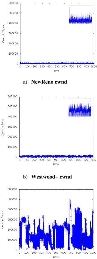
a) NewReno cwnd

b) Westwood+ cwnd

c) FTAT cwnd

(64)

The congestion window vs time graph (Figure 13) is helpful in confirming the congestion control behavior in different situations, for example NewReno reacts to a retransmission timeout (RTO) by resting the congestion window to one packet, while in the case of triple duplicate acknowledgement, NewReno halves the congestion window. Westwood+ reduces the congestion Window upon receiving three duplicate acknowledgements, by adjusting it to the last bandwidth measurement obtained, and FTAT starts new bandwidth measurement and enters the Adaptive Transmission which can identify a false alert of congestion and in that case, the congestion window increases. In case of congestion, FTAT reduces the congestion window to the available network bandwidth.

The cwnd graph of NewReno shows the behavior of the slow start and the congestion avoidance. Because of the long RTT and the loss rate, the window is going to one MSS more often, and it does not grow more than 12,000 bytes. On the other hand, Westwood shows more growth to the cwnd, also goes to one MSS more often, and the window does not grow more than 20,000 bytes. The cwnd of FTAT shows more growth even under the long RTT and the loss rate, the cwnd growth up to 500,000 Bytes, and goes to one MSS less often.

(65)

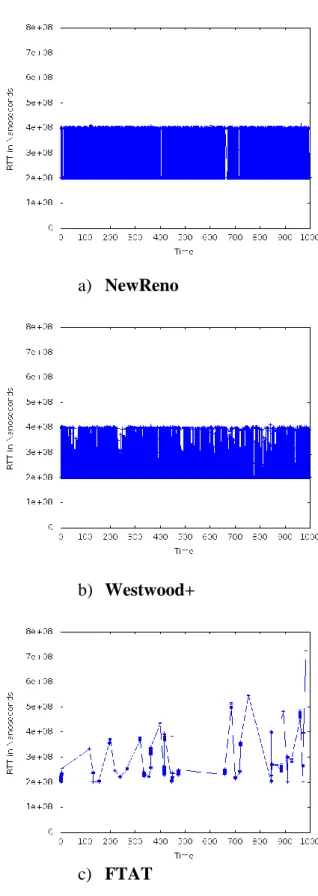
a) NewReno

b) Westwood+

c) FTAT Figure 14: RTT graphs for topology two