A NEW APPROACH FOR
FAST PROCESSING OF SPARQL QUERIES ON RDF QUADRUPLES
A DISSERTATION IN Computer Science
and
Telecommunications and Computer Networking
Presented to the Faculty of the University of Missouri-Kansas City in partial fulfillment of
the requirements for the degree
DOCTOR OF PHILOSOPHY
by
VASIL GEORGIEV SLAVOV
M.S., University of Missouri-Kansas City, 2012 B.A., William Jewell College, 2005
Kansas City, Missouri 2015
c 2015
VASIL GEORGIEV SLAVOV ALL RIGHTS RESERVED
A NEW APPROACH FOR
FAST PROCESSING OF SPARQL QUERIES ON RDF QUADRUPLES
Vasil Georgiev Slavov, Candidate for the Doctor of Philosophy Degree University of Missouri-Kansas City, 2015
ABSTRACT
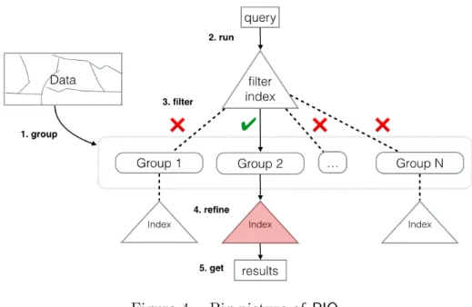
The Resource Description Framework (RDF) is a standard model for rep-resenting data on the Web. It enables the interchange and machine processing of data by considering its semantics. While RDF was first proposed with the vision of enabling the Semantic Web, it has now become popular in domain-specific applica-tions and the Web. Through advanced RDF technologies, one can perform semantic reasoning over data and extract knowledge in domains such as healthcare, biopharma-ceuticals, defense, and intelligence. Popular approaches like RDF-3X perform poorly on RDF datasets containing billions of triples when the queries are large and com-plex. This is because of the large number of join operations that must be performed during query processing. Moreover, most of the scalable approaches were designed to operate on RDF triples instead of quads. To address these issues, we propose to develop a new approach for fast and cost-effective processing of SPARQL queries on large RDF datasets containing RDF quadruples (or quads). Our approach employs a decrease-and-conquer strategy: Rather than indexing the entire RDF dataset, it
identifies groups of similar RDF graphs and indexes each group separately. During query processing, it uses a novel filtering index to first identify candidate groups that may contain matches for the query. On these candidates, it executes queries using a conventional SPARQL processor to produce the final results. A query optimization strategy using the candidate groups to further improve the query processing perfor-mance is also used.
APPROVAL PAGE
The faculty listed below, appointed by the Dean of the School of Computing and Engineering, have examined a dissertation titled ”A New Approach for Fast Processing of SPARQL Queries on RDF Quadruples,” presented by Vasil Georgiev Slavov, candidate for the Doctor of Philosophy degree, and certify that in their opinion it is worthy of acceptance.
Supervisory Committee
Praveen R. Rao, Ph.D., Committee Chair
Department of Computer Science Electrical Engineering Yugyung Lee, Ph.D.
Department of Computer Science Electrical Engineering Deep Medhi, Ph.D.
Department of Computer Science Electrical Engineering Vijay Kumar, Ph.D.
Department of Computer Science Electrical Engineering Appie van de Liefvoort, Ph.D.
CONTENTS
ABSTRACT . . . iii
LIST OF ILLUSTRATIONS . . . viii
LIST OF TABLES . . . x
ACKNOWLEDGMENTS . . . xi
Chapter 1. INTRODUCTION . . . 1
2. BACKGROUND AND MOTIVATIONS . . . 4
2.1.Semantic Web . . . 4
2.2.RDF . . . 6
2.3.SPARQL . . . 8
2.4.Related Work . . . 10
2.5.Motivations . . . 13
3. THE DESIGN OF RIQ . . . 15
3.1.Pattern Vectors . . . 16 3.2.Filtering Index . . . 20 3.3.Query Processing . . . 27 4. IMPLEMENTATION OF RIQ . . . 32 4.1.System Architecture . . . 32 4.2.Implementation . . . 36 4.3.Limitations . . . 37
5. EVALUATION . . . 40
5.1.Datasets . . . 41
5.2.Queries . . . 41
5.3.Indexing . . . 42
5.4.Query Processing . . . 45
6. CONCLUSION AND FUTURE WORK . . . 61
Appendix A. QUERIES . . . 63 A.1.LUBM Queries . . . 64 A.2.BTC-2012 Queries . . . 75 B. SPARQL GRAMMAR . . . 85 REFERENCES . . . 87 VITA . . . 93
ILLUSTRATIONS
Figure Page
1. Linking Open Data cloud . . . 5
2. The Semantic Web stack . . . 7
3. An example of a SPARQL query . . . 8
4. Big picture of RIQ . . . 15
5. Pattern Vectors of RIQ . . . 16
6. Grouping of similar PVs in RIQ . . . 22
7. Grouping five PVs into two connected components . . . 23
8. LSH: probability vs similarity . . . 24
9. Bloom filter test operation . . . 25
10. An example of a BGP Tree . . . 29
11. The BGP Tree after pruning . . . 29
12. Architecture of RIQ . . . 32
13. Filtering Index generation in RIQ . . . 33
14. Query execution in RIQ . . . 35
15. Query processing times for LUBM, large queries . . . 56
16. Query processing times for BTC-2012, large queries . . . 57
17. Query processing times for LUBM, small queries . . . 58
18. Query processing times for BTC-2012, small queries . . . 59
20. Visual representation of LUBM query L1 with a large, complex BGP . . 66 21. Visual representation of LUBM query L2 with a large, complex BGP . . 67 22. Visual representation of LUBM query L3 with a large, complex BGP . . 69 23. Visual representation of BTC query B1 with a large, complex BGP . . . 76 24. Visual representation of BTC query B2 with a large, complex BGP . . . 78
TABLES
Table Page
1. Transformations in RIQ . . . 17
2. Queries for LUBM and BTC-2012. . . 43
3. RIQ’s indexing performance: construction time . . . 45
4. RIQ’s indexing performance: settings and size . . . 45
5. Filtering time for RIQ on LUBM. . . 46
6. Filtering time for RIQ on BTC-2012. . . 46
7. Fastest approach for processing queries over LUBM. . . 50
8. Fastest approach for processing queries over BTC-2012. . . 50
9. Geometric Mean of the query processing times for LUBM . . . 51
10. Geometric Mean of the query processing times for BTC-2012 . . . 51
11. Query processing times for LUBM . . . 52
12. Query processing times of LSH and Jaccard using RIQ for LUBM . . . . 53
13. Query processing times for BTC-2012. . . 54
14. Query processing times of LSH and Jaccard using RIQ for BTC-2012 . . 54
ACKNOWLEDGMENTS
I would like to thank my dissertation advisor Dr. Praveen Rao. Without his guidance, support, motivation and extreme patience, this work would not have been possible. My experience in working with him on this and other research projects inspired and motivated me to continue my academic career after completing my MS degree and pursue a Ph.D. degree in Computer Science. Dr. Rao supported me financially which allowed me to dedicate all of my time to research. I would also like to to thank Anas Katib for the very valuable contributions he made to this project and all the work he did as a co-author for the paper submissions on this topic. Finally, I want to thank my family for their support throughout the years I have been in school. This work was supported by the National Science Foundation under Grant No. 1115871.
CHAPTER 1 INTRODUCTION
The Resource Description Framework (RDF) has become a widely used, stan-dardized model for publishing and exchanging data [10]. From research institutions and government agencies [1, 2], to large media companies [41, 8] and retailers [4], RDF has been adopted and used in production environments at a scale which was only dreamed of in the initial stages of the development of the Semantic Web vision of Tim Berners-Lee [12].
The most popular use case for RDF is Linked Data, a set of technologies and specifications for publishing and interconnecting structures data on the Web in a machine-readable and consumable way [24].
In addition to the increased popularity of RDF technologies, a number of very large RDF datasets (e.g. Billion Triples Challenge (BTC) [11] and Linking Open Government Data (LOGD) [6]) have pushed the limits of scalability in terms of indexing and query processing. Both BTC and LOGD are non-synthetic datasets which have long surpassed the billion-quad mark and contain millions of RDF graphs. Researchers in both the Database and the Semantic Web communities have proposed scalable solutions for processing large RDF datasets [17, 59, 47, 19, 37, 25, 63, 64], but all of those approaches have been evaluated using datasets containing RDF triples. The RDF quadruples contained in more recent, larger datasets extend the idea of the RDF triple by adding a context/graph name to the traditional subject,
predicate, object statement. The context names the graph to which the triple belongs and enables the use of the SPARQL’s 1.1 GRAPH keyword [13] to match a specific graph pattern within a single RDF graph among millions of individual graphs in a large RDF dataset. Simply ignoring the context of a quad is not possible, as we show in the following chapters, because it yields incorrect results.
In addition to not supporting RDF quadruples, none of the state-of-the-art so-lutions have been evaluated using SPARQL queries containing large, complex graph patterns (e.g. with a large number of triple patterns and/or undirected cycles). In fact, in the following pages, we show that those approaches yield very poor perfor-mance on SPARQL queries with large, complex graph patterns. One of the reasons for the poor performance is the large number of join operations which must be done during query processing. In the evaluation we performed, any approach which first finds matches for subpatterns in a large graph pattern and then merges partial results with join operations does not scale to billion-quad datasets.
We propose a new approach for fast processing of SPARQL queries on RDF quads called RIQ (RDF Indexing on Quadruples). The contributions of this work are:
• A new vector approach for representing RDF graphs and SPARQL queries which captures the properties of both triples in a graph and triple patterns in a query. • A new filtering index which groups similar RDF graphs using Locality Sensi-tive Hashing [38] and a combination of Bloom Filters and Counting Bloom Filters [28] for compact storage.
filtering index to process SPARQL queries efficiently by identifying candidate groups of RDF graphs which may contain a match for a query without false dismissals.
• A comprehensive evaluation of RIQ on a synthetic and a real RDF dataset containing about 1.4 billion quads each with a large number of queries and com-pared against state-of-the-art approaches such as RDF-3X [46], Jena TDB [18] and Virtuoso [31].
The rest of this work is organized as follows. Chapter 2 provides the back-ground on Semantic Web focusing on RDF and SPARQL. It also describes the related work and the motivation for our work. Chapter 3 describes the design of RIQ, start-ing with an in-depth introduction to the new vector representation of RDF graphs and continuing with the generation of a filtering index and the role it plays during query processing. Chapter 4 covers the implementation of RIQ and highlights some of the limitations of this approach. Chapter 5 reports the results of the comprehensive evaluation of RIQ. Finally, we conclude in Chapter 6.
CHAPTER 2
BACKGROUND AND MOTIVATIONS 2.1 Semantic Web
The term Semantic Web was invented by Tim Berners-Lee, the inventor of the World Wide Web. In simple terms, the Semantic Web refers to the web of data which can be processed by machines [57]. The W3C, the standard organization behind the WWW, the Semantic Web and many other web technologies, defines it as a common framework designed for data sharing and re-usability across applications and enterprises [16]. There has been some confusion regarding the relationship between the Semantic Web and another term closely related to it, Linked Data. The most common view is that the ”Semantic Web is made up of Linked Data” [5] and that ”the Semantic Web is the whole, while Linked Data is the parts” [5]. According to Tim Berners-Lee, Linked Data is ”the Semantic Web done right” [22].
Linked Data refers to the set of technologies and specifications or best practices used for publishing and interconnecting structured data on the Web in a machine-readable and consumable way [24]. The main technologies behind Linked Data are URIs, HTTP, RDF and SPARQL. URIs are used as names for things. HTTP URIs are used for looking up things by machines and people (retrieving resources and their descriptions). RDF is the data model format of choice. SPARQL is the standard query language. In essence, Linked Data enables connecting related data across the Web using URIs, HTTP and RDF.
Figure 1. Linking Open Data cloud
(Source: by Richard Cyganiak and Anja Jentzschhttp://lod-cloud.net/)
••
Linked Data is a popular use case of RDF on the Web; it has a large col-lection of different knowledge bases, which are represented in RDF (e.g., DBpedia, Data.gov [6]). With a growing number of new applications relying on Semantic Web technologies (e.g., Pfizer [9], Newsweek, BBC, The New York Times, Best Buy [4]) and the availability of large RDF datasets (e.g., Billion Triples Challenge (BTC) [11], Linking Open Government Data (LOGD) [6]), there is a need to advance the state-of-the-art in storing, indexing, and query processing of RDF datasets. The Linking Open Data (LOD) [42] cloud diagram shown in Figure 1 visualizes the datasets which have been published in Linked Data format. As of this writing, there were 570 datasets published. The size of the circles corresponds to the size of the datasets and the largest circles indicate datasets which exceed 1 billion triples.
The Semantic Web encompasses a number of different technologies and speci-fications. Figure 2 identifies most of them: they range from low-level hypertext web technologies (IRI, Unicode, XML), through standardized Semantic Web technologies (RDF, RDFS, OWL, SPARQL), to unrealized Semantic Web technologies (cryptog-raphy, user interfaces) [15]. In this work, we are going to focus on the middle layer: the standardized Semantic Web technologies RDF [10] and SPARQL [14].
2.2 RDF
The Resource Description Framework (RDF) is a widely used model for data interchange which has been standardized into a set of W3C specifications [10]. RDF is intended for describing web resources and the relationships between them. RDF expressions are in the form of subject-predicate-object statements. These statements
Figure 2. The Semantic Web stack
(Source: http://en.wikipedia.org/wiki/Semantic_Web_Stack)
set:
(U ∪B)×U×(U ∪L∪B)
where U are URIs, L are literals and B are blank nodes and all three are disjoint sets. An RDF term is U ∪L∪B. An RDF element is any subject, predicate or object [40].
Blank nodes are used to identify unknown constants. Blank nodes are useful for making assertions where something is an object of one statement and a subject of another. For example, the director of X is Godard and the year of X is 1970. A query can be issued for what Godard directed in 1970 andX will be the result.
Resources are uniquely identified using URIs (Uniform Resource Identifiers). Resources are described in terms of their properties and values. A group of RDF statements can be visualized as a directed, labeled graph. The source node is the
~ld.bc·~~J S·" ~'h'-~"""" H>1~·I.,t\'i, ~'h'-,,""""
r
-r
..
~,, -I
M-=.
I
1
.
Jrr""",,,,
oW ""h'~cgo,BGP 1 BGP 2 BGP 3 BGP 4 BGP 5 SELECT * WHERE { GRAPH ?g {
{ ?city onto:areaLand ?area . UNION
{ ?city onto:timeZone ?zone .
?city onto:abstract ?abstract . } ?city onto:country res:United_States . ?city onto:postalCode ?postal .
FILTER EXISTS { ?city onto:utcOffset ?offset . } OPTIONAL { ?city onto:populationTotal ?popu . } }}
?city onto:areaCode ?code . }
Figure 3. An example of a SPARQL query
subject, the sink node is the object, and the predicate/property is the edge. Quads extend the idea of triples by adding a fourth entity called a context. The context names the graph to which the triple belongs. Triples with the same context belong to the same graph. RDF data my be serialized in a number of different formats, but the most common ones are RDF/XML, Notation-3 (N3), Turtle (TTL), NTriples (NT), NQuads (NQ).
2.3 SPARQL
SPARQL is the standard query language for RDF data. The fundamental operation in RDF query processing is Basic Graph Pattern Matching [13]. A Basic Graph Pattern (BGP) in a query combines a set of triple patterns. BGP queries are a conjunctive fragment which expresses the core Select-Project-Join paradigm in database queries [40]. The SPARQL triple patterns (s, p, o) are from the set:
where U are URIs, L are literals, B are blank nodes, and V are variables [40]. The variables in the BGP are bound to RDF terms in the data during query processing via subgraph matching [13]. Join operations are denoted by using common variables in different triple patterns. SPARQL’sGRAPHkeyword [13] can be used to perform BGP matching within a specific graph (by naming it) or in any graph (by using a variable for the graph name). GRAPH queries are used on RDF quadruples which contain the context/graph to which a particular triple belongs. Figure 3 shows an example of such a query.
There are three main types of SPARQL queries. The first type is star-join queries. Those queries have the same variable in the subject position (e.g. ?x type :artist . ?x :firstName ?y . ?x :paints ?z .). The second most com-mon type are the path or chain queries where the object of each pattern is joined with the subject of the next one (e.g. ?x :paints ?y. ?y :exhibitedIn ?z . ?z :locatedIn :madrid .) [40]. Finally, more complex SPARQL queries which can be typical for real-world usage, may contain undirected cycles [53] (e.g. ?a :p ?b . ?b :q ?c . ?a :r ?c .).
In terms of selectivity and join results, queries may be categorized in three different groups [19]. The first group is queries which contain highly selective triple patterns (e.g. ?s :residesIn USA . ?s :hasSSN "123-45-6789" .). The second group consists of queries with triple patterns with low-selectivity, but which gen-erate few results. Those queries are also known as highly selective join queries (?s :residesIn India . ?s :worksFor BigOrg .). Finally the third group of SPARQL queries contains low-selectivity triple patterns and low-selectivity join
re-sults (e.g. ?s :residesIn USA . ?s :hasSSN ?y .) [19]. 2.4 Related Work
Since the early vision of the Semantic Web in 2001 [12], many approaches have been developed for indexing and querying RDF data. Overall, there are two storage and query processing categories of RDF solutions: centralized and distributed. Because RIQ is a centralized approach, we are only going to focus on this category. Within the centralized solutions, there are four major groups of applications: triple stores, vertically partitioned tables, property tables, and specialized systems [36]. Some of these systems have originated in the Semantic Web community such as Jena [62] and Sesame [29], others have started in the database community such as SW-Store [17], RDF-3X [46], and Hexastore [59].
2.4.1 Triple stores
Triple stores store RDF triples in a three-column table. Additional indexes and statistics are also maintained. Entities from the triples (constants, properties, resource identifiers) are converted to numerical ids. The most prominent examples of triple store RDF solutions are RDF-3X [46], Hexastore [59], and DB2RDF [25] from the database community and 3store [33], and Virtuoso [31] from the Semantic Web community.
RDF-3X is one of the most popular centralized RDF processing research appli-cations [46, 47, 48]. While RDF-3X has been able to scale remarkably well throughout the years considering that active development has stopped, it is missing support for some more recent RDF and SPARQL specifications. The most glaring omission is
support for quads. While RDF-3X is considered a triples store, it never actually maintains a single triples table, but rather builds clustered B+ tree indexes on all six combinations of subject-predicate-object triples. RDF-3X also makes use of six addi-tional aggregate indexes, one for each possible pair of (s, p, o) triples and each order. Furthermore, RDF-3X is able to keep the size of the index small by encoding strings into ids and by compressing the leaves of the B++ tree indexes in pages [36]. At query time, RDF-3X uses a new join ordering method based on selectivity estimates based on statistics it maintains.
Virtuoso employs space-optimized mapping to identifiers. Only long IRIs as converted to IDs, otherwise the text of each RDF term is stored. Virtuoso creates a GSPO quad table with a primary index on all four (graph, subject, predicate, object) attributes. Virtuoso also creates a bitmap OGPS index. It builds a bit-vector of each OGP combination where the bit position for each subject is set to one for each OGP bit-vector in the data. In order to make its indexes more compact, Virtuoso eliminates common prefixes and strings. Further, it compresses each page [31].
During query processing, Virtuoso resolves simple joins by calculating the conjunction of sparse bit vectors by finding their intersection. Virtuoso does not use pre-calculated statistics for cost estimation. It employs query-time sampling and makes these estimates on the fly [36].
2.4.2 Vertically Partitioned Tables
Vertically partitioned tables maintain one table for each property. They exploit the fact that most RDF datasets contain a fixed number of properties. Vertically partitioned tables are also known as horizontal (binary) table stores [51]. The columns
in each property table are limited only to subjects and objects, and an optional graph id if RDF quadruples are being stored. Column stores use ids for each column entry and reconstruct the row at query time. While vertically partitioned tables are efficient for triple patterns with fixed properties, they are very expensive for triple patterns with a property variable because of the need to access all 2-column tables. [36]. These very narrow tables can then be stored in a column store. Because the entries in each column have the same type, the tables can be efficiently compressed. The most popular example of a vertically partitioned table is SW-Store [17].
2.4.3 Property Tables
Property tables exploit the fact that a large number of subjects have the same predicate. Subjects with similar predicates are grouped together in the same table. The goal is to reduce self-joins. The effect is that queries with those properties are more efficient, but extra work is required for subjects without those properties or subjects with many objects for the same property. Two examples of this approach are Oracle’s RDF storage implementation [30] and the Apache Jena project [61]. Apache Jena TDB is the persistent graph storage layer for Jena. The first edition of Jena was a SQL-based system. Jena TDB exploits memory-mapped I/O on 64-bit hardware instead of using a custom caching mechanism [49]. Jena TDB creates three composite B+ tree indexes: SPO, POS, OSP. It does not create a triple table; instead, all three indexes contain a subject, a predicate, and an object. On one hand, this avoids full table scans at query time when doing triple matching. But on the other, this increases loading time significantly. The evaluation Chapter 5 shows this when
serve as references in a node table created during indexing. Part of Jena’s claim to fame is the significant performance improvements it is able to achieve compared to its competitors when reading and/or writing the translation node table [49].
BGP matching in Jena TDB is done by choosing the most matching index. If the query triple pattern has a known S and P, the SPO index is used. Next, a range scan is performed to find the node ids of the unknown triple pattern terms (the variables). The node id to RDF term is left for the very last step and is only performed on actual result triples.
2.4.4 Specialized and Distributed Systems
Finally, a number of diverse and specialized systems use their own, unique techniques for storing RDF data. BitMat [19] manages to process queries with low selectivity triple patterns which produce large intermediate join results quickly by performing in-memory processing of bit matrices. Others exploit the graph properties of RDF data [58, 26, 65]. Unfortunately, these techniques have not been tested against larger RDF datasets of more than 50 million triples. Distributed/parallel RDF query processing has gained popularity in more recent research [37, 64], however, our approach focuses on localized and centralized RDF query processing.
2.5 Motivations
We motivate our work with two key observations. The first one is that the approaches outlined in the related work above were designed for processing of RDF triples, not quadruples. While it is possible to ignore the context in a quad, it is certainly not desirable because the likelihood of incorrect results is very high due to
bindings to a BGP from different RDF graphs. For example, let us consider two quads which belong to two different graphs: <a> <b> <c> <g1> . <a> <b> <e> <g2> . If we index these quads with an approach which supports only triples, such as RDF-3X, and issue the following query SELECT ?x WHERE { GRAPH ?g { ?x <b> <c> . ?x <b> <e> . } } , we would get <a> as the result. However, a quad store will return an empty result set which is the correct result as there is no single graph which contains both triple patterns (there are two graphs containing partial matches). Because the triple store approach ignores the name of the graph, it treats both triple patterns as if they belong to the same graph.
The second motivation for this work is the relatively simple queries used in the evaluations of the approaches outlined above. The queries used usually contain few triple patterns (no more than 8) and are either star-shaped or contain very short paths/chains. None of the state-of-the-art techniques for RDF query processing have investigated processing SPARQL queries with large and complex BGPs. For example, queries containing undirected cycles such as this one: ?a <p> ?b . ?b <q> ?c . ?a <r> ?c . have not been evaluated. We believe that those types of queries are more realistic for real-world SPARQL usage as they more closely mirror the complex SQL queries used in the relational world.
CHAPTER 3 THE DESIGN OF RIQ
In this section, we are going to describe the design of RIQ and its components. We are going to discuss in detail the way RIQ performs indexing of RDF data and query processing of SPARQL queries. We are going to focus on the novel vector ap-proach for representing RDF graphs and queries, the new filtering index contribution which is at the heart of RIQ, and we are going to conclude with the new decrease & conquer approach which RIQ takes during query processing.
?PO S?O SP? S?? ?P? ??O SPO H((s,p,o)) H((?,p,o)) H((s,?,o)) H((s,p,?)) H((s,?,?)) H((?,p,?)) H((?,?,o))
res:Oswego onto:country res:United_States <http://..../Oswego.xml> quad
p o c
s
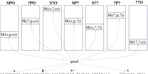
Figure 5. Pattern Vectors of RIQ
3.1 Pattern Vectors
One of the main contributions of this work is a new vector representation of RDF graphs and BGPs. We call this new representation Pattern Vectors (or PVs for short). Pattern Vectors allow us to capture the properties of triples in RDF data and triple patterns in SPARQL query BGPs. Pattern Vectors are an essential part of RIQ and play a central role in all phases of RDF indexing and query processing.
Before describing the design and use of Pattern Vectors, let us define some prerequisite essential transformations of RDF graphs and BGP patterns. First, let’s define the set of canonical patterns as P = {SP O, SP?, S?O, ?P O, S??, ?P?, ??O}. The setP represents all the possible permutations of the subject, the predicate, and the object, or their substitution by a variable in a triple or a triple pattern. The transformation of a triple, we denote as fD : P× {(s, p, o)} → OD. We show the
range, OD, in Table 1. Note that OD resembles a BGP triple pattern with excluded T 1 1\ T
'\
//'
1
//
\
~
j . . . . ....
\. . . . . . . .. . ---...
--
. . -_ _ _ _ _ _ _ _ _ '~ I "'-- .. - .- ~.Table 1. Transformations in RIQ Transformation fD Transformation fQ fD(SPO, (s,p,o)) = (s,p,o) fQ(‘s p o’) = (SPO,(s,p,o)) fD(SP?, (s,p,o)) = (s,p,?) fQ(‘s p ?vo’) = (SP?,(s,p,?)) fD(S?O, (s,p,o)) = (s,?,o) fQ(‘s ?vp o’) = (S?O,(s,?,o)) fD(?PO, (s,p,o)) = (?,p,o) fQ(‘?vs p o’) =(?PO,(?,p,o)) fD(S??, (s,p,o)) = (s,?,?) fQ(‘s ?vp ?o’) = (S??,(s,?,?)) fD(?P?, (s,p,o)) = (?,p,?) fQ(‘?vs p ?vo’) = (?P?,(?,p,?)) fD(??O, (s,p,o)) = (?,?,o) fQ(‘?vs ?vp o’) = (??O,(?,?,o))
variable names.
Next, we denote the transformation of a BGP triple pattern asfQ :T →P×OQ
where T denotes the set of triple patterns which may appear in a SPARQL query. We show the range, P×OQ, in Table 1 which denotes the canonical pattern of a given
BGP triple pattern. Note that fQ(’s p o’) is a valid transformation (even though
it has no variables) because SELECT ?g WHERE { GRAPH ?g { s p o .} } is a valid SPARQL 1.1 query.
The purpose of both transformations is to allow us to map both the RDF data and the SPARQL queries to a common reference point which will let us perform different operations on both. In particular, we will be able to test if a triple is a match for a BGP triple pattern.
Having defined the essential transformations, let us introduce Pattern Vectors. Given an RDF graph which consists of triples with the same context c, we create a vector representation of the graph which we call a Pattern Vector (PV). We denote this PV as Vc. Pattern Vectors consist of 7 separate vectors, one for each r∈P: Vc
Algorithm 1Construction of the PV of an RDF graph Require: An RDF graph G with context c
Ensure: PV Vc 1: for each (s, p, o, c)∈G do 2: for each r∈P do 3: insert H(fD(r,(s, p, o))) into Vc,r 4: for each r∈P do 5: sort Vc,r 6: return Vc
= (Vc,SP O, Vc,SP?, Vc,S?O, Vc,?P O, Vc,S??, Vc,?P?, Vc,??O). Figure 5 shows an example
of a Pattern Vector and the mapping between a triple and the 7 vectors in the PV. The individual vectors Vc,r consist of the non-negative integer output of the hash
function H: B → Z∗ where B is the original triple represented as a bit string. We
compute H(fD(r,(s, p, o))) for each r ∈P. The required space for each Vc is linear
to the number of quads in the graph. Algorithm 1 describes the construction of the Pattern Vector of an RDF graph.
We base the hash functionH on Rabin’s fingerprinting technique [50]. Rabin’s fingerprinting technique is efficient to compute and the probability for collision is very low. The hash values we generate are 32-bit unsigned integers. The irreducible polynomial is of degree 31. Given these values, the probability of collision is 2−20 [27]. Because all the triples in one RDF graph are unique (by design), the vector Vc,SP O is
a set of the non-negative integer outputs of H. However, when we start substituting the elements of each triple with variables, the bit string inputs to H are no longer unique and therefore, the remaining Vc vectors are multisets.
Start-Algorithm 2Construction of the PV of a BGP Require: A BGP q
Ensure: TPV Vq
1: for each triple pattern t ∈Q do 2: (r, oq)←fQ(t)
3: insert H(oq) into Vq[r]
4: return Vq
ing with an empty Vq,r, we compute fQ(t) for each triple pattern t and produce a
pair (r, o) where r is the canonical pattern for t and o is the input bit string for H. We insert the output of H into Vq,r. Similarly to the Pattern Vector generation for
RDF graphs, Vq consists of one set (Vq,SP O) and six multisets because different triple
patterns containing variables may hash to the same value. While we ignore the ?s ?p ?o triple pattern during PV construction, we consider it during query processing when we execute the optimized queries. Algorithm 2 describes the construction of the Pattern Vector of a BGP.
In order to accomplish the goal of grouping similar RDF graphs together, we define two operations on Pattern Vectors which let us group similar PVs together. (Grouping of similar RDF graphs helps us quickly identify candidate RDF graphs at query time.) The definitions of the Union and Similarity operations follow:
DEFINITION 3.1 (Union). Given two PVs, say Va and Vb, their union Va∪Vb is
a PV say Vc, where Vc,r ←Va,r∪Vb,r and r ∈P.
DEFINITION 3.2 (Similarity). Given two PVs, say Va and Vb, their similarity is
denoted by sim(Va, Vb) = max
r∈P sim(Va,r, Vb,r), where sim(Va,r, Vb,r) =
|Va,r∩Vb,r|
3.2 Filtering Index
As described in the previous section, both RDF graphs and BGPs are mapped to their respective Pattern Vectors. This enables us to perform operations such as the Union and Similarity operations defined above. A key necessary condition which connects the two types of Pattern Vectors and is at the heart of RIQ’s indexing and query processing is defined and proved below. This condition is concerned with processing BGPs via subgraph matching at query time.
THEOREM 3.3. Suppose Vc and Vq denote the PVs of an RDF graph and a BGP,
respectively. If the BGP has a subgraph match in the RDF graph, then V r∈P
(Vq,r ⊆ Vc,r) = TRUE.
We assume that the BGP q denotes a connected graph. Because q has a subgraph match in the graph, every triple pattern in q has a matching triple in the graph. Consider a triple pattern t in q. Let (r, o)←fQ(t). During the construction
of Vq, we inserted H(o) into Vq,r. Suppose d denotes the matching triple pattern
for t in the graph. During the construction of Vc, we had inserted H(fD(r, d))
into Vc,r. Also, H(o) = H(fD(r, d)). Therefore, elements in Vq,r have a
one-to-one correspondence with a subset of elements in Vc,r. Hence, Vq,r ⊆Vc,r. This is true
for every r ∈P, and hence, V r∈P
(Vq,r ⊆Vc,r) = TRUE.
Theorem 3.3 enables us to identify the RDF graphs for which a BGP satisfies the necessary condition. Those graphs represent a superset of the actual graphs which contain a subgraph match for the BGP. Since the candidate graphs are a superset, there will be no false dismissals.
In order to eliminate the need for exhaustively testing each Pattern Vector for every BGP during query processing, we have developed a novel filtering index called PV-Index for organizing and processing the millions of Pattern Vectors which represent the RDF graphs. The goal of the PV-Index is to quickly and efficiently identify the candidate RDF graphs. To speed up query time, the PV-Index’s role is to discard a large number of RDF graphs without false dismissals.
There are two challenges in developing the PV-Index. The first one is grouping of Pattern Vectors in such a way that discarding of non-matching PVs is possible. The second is minimizing the query processing I/O by designing the PV-Index to store the PVs compactly. The first issue we solve by using Locality Sensitive Hashing (LSH) [38]. LSH has been employed for similarity on sets based on the Jaccard index [35]. Given a set S, LSHk,l,m(S) is computed by picking k×l random linear
hash functions. The functions are the of the form h(x) = (ax+b) mod u where
u is a prime and a and b are integers such that 0 < a < u and 0 ≤ b < u. Next, we go over all the items of the set S and compute g(S) = min{h(x)}. Using Rabin’s fingerprinting technique [50], we hash each group of l hash values to the range [0, m−1] and we get k hash values for the set S. The main reason for using LSH on sets is that given two sets S1 and S2, p =
|S1∩S2|
|S1∪S2|, Pr[g(S1) = g(S2)] = p.
Furthermore, the probability that LSHk,l,m(S1) and LSHk,l,m(S2) have at least one
identical hash value is 1−(1− pl)k. Note that all these properties are valid for multisets as well. Figure 8 shows the way the probability for collision changes based on the similarity of the input for different value of k and l.
Figure 6. Grouping of similar PVs in RIQ
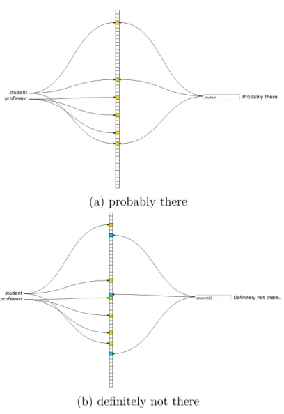
In order to compactly represent the PV-Index, we make use of Bloom filters (BFs) and Counting Bloom Filters (CBFs) [28]. Bloom filters are a probabilistic data structure which is used for representing a set of items and for testing the membership in that set. They support two operations: add and test. Bloom filters are usually implemented as bit vectors and k different hash functions are used for adding an element to the set. Counting Bloom filters use n-bit counters instead. The test operation’s output is either definitely not in the set or may be is in the set. The probability for false positives is approximately (1−e−kn/m)k where m is the length
of the bit vector, k is the number of hash functions and n is the number of items added to the Bloom filter. It is not possible to remove items from the set because that would introduce false negatives. Given a predetermined capacity of a Bloom filter (the number of elements to be inserted) and a desired false positive rate, the number of hash functions and the size of the bit vector used can easily be calculated. Figure 9 shows examples of testing a Bloom filter for existing and non-existing elements.
-
..
-'"'
...
•
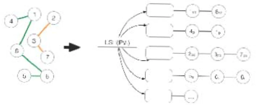
Va V b Vc Vd Ve LSH Vc,S?O {2,8} LSH Vb,?P? {1,7} LSH Vd,?P? {4,7} LSH Ve,?P? {4,9} LSH Va,S?O {2,5} 2 4 7
Figure 7. Grouping five PVs into two connected components shown in red and blue (k = 2, m= 10)
Algorithm 3 outlines the construction of the PV-Index. The first step is build-ing a graph G whose vertices represent the individual Pattern Vectors (which rep-resent the input RDF graphs). LSH is applied on each of the seven vectors of the PV 6. If after applying LSH, there is at least one identical hash value for the same pattern r of two different PVs, we draw an edge between the vertices of those two PVs (Lines 2 to 8). This means that two Pattern Vectors are dissimilar with high probability if there is not edge between them. The second step is computing the connected components in the graph G in linear time using breadth-first search [43]. Individual connected components in G represent RDF graphs whose Pattern Vectors are similar with high probability. All the RDF graphs in a connected component are treated as one group and the union of their PVs is computed (Line 11) using the Union operation defined previously in this section. Note that the Union operation both sum-marizes the PVs and preserves the necessary condition in Theorem 3.3. Futhermore, the Union operation can be performed in linear time because the individual vectors in each PV are kept sorted.
Figure 8. LSH: probability vs similarity
We use a combination of Bloom filters (BFs) and Counting Bloom filters (CBFs) to represent the union of PVs in each connected component. For the SPO canonical pattern, we use a Bloom filter because that vector is a set. We use Count-ing Bloom filters for the vectors of the other six canonical patterns because they are multisets. We set the capacity (the number of elements to be inserted) and the false positive rate for filter (Lines 12 and 13) where the capacity is equal to the cardi-nality of the vector. We also store the ids of the graphs belonging to a particular connected component (Line 14). The collection of all BFs and CBFs make up the PV-Index. In addition to constructing the PV-Index, each group of similar graphs is indexed with an RDF application such as RDF-3X, Jena TDB or Virtuoso.
(a) probably there
(b) definitely not there
Figure 9. Bloom filter test operation
Algorithm 3The PV-Index Construction
Require: a list of PVs; (k, l, m): LSH parameters; : false positive rate Ensure: filters of all the groups of similar RDF graphs
1: Let G(V,E) be initialized to an empty graph 2: for each PV V do
3: Add a new vertex vi to V
4: for each r∈P do
5: {hi1, ..., hik} ←LSHk,l,m(Vr)
6: for every vj ∈V and i6=j do
7: if ∃ o s.t. 1≤o ≤k and hio =hjo then
8: Add an edge (vi, vj) to E if not already present
9: Compute the connected components of G. Let {C1, ..., Ct} denote these
compo-nents.
10: for i= 1 to t do
11: Compute the union Ui of all PVs corresponding to the vertices in Ci
12: Construct a BF for Ui,SP O with false positive rate given the capacity |Ui,SP O|
13: Construct a CBF for each of the remaining vectors of Ui with false positive
rate given the capacity |Ui,∗|
14: Store the ids of graphs belonging to Ci
3.3 Query Processing
We take adecrease & conquerapproach to processing SPARQL queries in RIQ. First, using the PV-Index, we identify candidate groups of RDF graphs which with high probability might contain a match for the BGPs in the query. Next, we execute the optimized (and potentially re-written) SPARQL queries only on those candidates and skip a large number of groups without false dismissals.
We start by parsing the given SPARQL query’s GRAPH block based on the supported SPARQL grammar (Appendix B). We generate a parse tree which we call the BGP Tree. The BGP Tree serves as the query execution plan for processing the individual BGPs. Figure 10 shows an example of such a parse tree. Algorithm 4 shows the pseudo-code for the evaluation of the BGP tree. We maintain the status of the evaluation of each connected component (group of RDF graphs) of the PV-Index by keeping track of it in a variable called eval[n] where n is the id of the node. We initialize eval for all nodes to FALSE. In depth-first order, we invoke Algorithm 4 on each connected component and recursively process the individual nodes in a connected component. We skip children of GroupGraphPatternSub which evaluate to FALSE (Line 4). This is a part of the query optimization technique and is possible because it is certain that the RDF graphs in that particular connected component will not produce for the subexpressions rooted at that node. However, subexpressions rooted atGroupOrUnionGraphPattern will evaluate to TRUEif at least one of their children evaluate to TRUE (Line 7).
We test the necessary condition defined in Theorem 3.3 upon reaching a leaf node which is a BGP (a TriplesBlock and call Algorithm 5. In this algorithm, we
have to construct query PVs on the fly (Line 2) because the capacity of the data PVs varies and comparing BFs and CBFs (Line 3) with different capacities in order to establish if one is a subset of the other is meaningless. Finally, back in Algorithm 4, if an OptionalGraphPattern node evaluates to TRUE, we return TRUE because of the semantics of OPTIONAL in SPARQL. A connected component (a group of RDF graphs) is considered a candidate if the root of the tree (eval[n]) evaluates to TRUE. Once a group of RDF graphs is identified as a candidate, we are able to generate an optimized SPARQL query by traversing the BGP Tree and pruning parts of it based on Algorithm 6. For certain predicates such as FILTER, we include all of the subpredicates they include (e.g. NOT EXISTS). In order to be able to combine the results from multiple candidates successfully, we have to project all the variables from the original query, even if they no longer appear in the optimized query due to pruning of the BGP which contained those variables. Figure 11 shows an example of a optimized SPARQL query generated after running the pruning algorithm. Note that both the OPTIONAL and the UNION blocks are absent. Excluding those BGPs during query execution can significantly speed up query time as shown in Chapter 5. Finally, we execute the optimized SPARQL query on the candidates graphs by using an application such as Jena TDB or Virtuoso. The results of the output from all the candidates are combined in a trivial manner as no graphs span between candidate groups.
4 BGP BGP3 BGP1 BGP2 BGP5 GroupGraphPatternSub GroupGraphPattern GraphPatternNotTriples GroupGraphPatternSub GroupGraphPattern Filter Constraint BuiltInCall ExistsFunction TriplesBlock EXISTS FILTER GraphPatternNotTriples UNION GroupGraphPatternSubList TriplesBlock GroupGraphPatternSubList T T T T T T T T T T T T T T T T T T GroupGraphPatternSub TriplesBlock GroupGraphPattern GroupGraphPatternSub TriplesBlock GroupGraphPattern GraphOrUnionGraphPattern T T T F F F GroupGraphPatternSubList GraphPatternNotTriples OptionalGraphPattern GroupGraphPatternSub GroupGraphPattern T F F OPTIONAL F T TriplesBlock F T
Figure 10. An example of a BGP Tree
4 BGP BGP3 BGP1 GroupGraphPatternSub GroupGraphPattern GraphPatternNotTriples GroupGraphPatternSub GroupGraphPattern Filter Constraint BuiltInCall ExistsFunction TriplesBlock EXISTS FILTER GraphPatternNotTriples GroupGraphPatternSubList TriplesBlock GroupGraphPatternSubList T T T T T T T T T T T T T T T T GroupGraphPatternSubList GraphPatternNotTriples T T GroupGraphPatternSub TriplesBlock GroupGraphPattern T T T GraphOrUnionGraphPatternT
Algorithm 4EvalBGPTree(node n, conn. component j) 1: Let c1, ..., cτ denote the child nodes of n (left-to-right)
2: for i = 1 to τ do
3: eval[ci] ← EvalBGPTree(ci, j)
4: if n is GroupGraphPattern& eval[ci] = FALSE then
5: eval[n] ← FALSE
6: return FALSE {//skip rest of the nodes} 7: if n is GroupOrUnionGraphPattern then 8: eval[n]← τ W i=1 eval[ci]
9: else if n is EXISTS then 10: eval[n]←eval[c1]
11: else if n isNOT EXISTS then 12: eval[n]← TRUE
13: else if n isPredicate then
14: eval[n]← TRUE{//skip processing predicates} 15: else if n isBGP then
16: Let q denote the basic graph pattern 17: eval[n] ← IsMatch(q, j) 18: else 19: eval[n]←eval[cτ] 20: if n isOptionalGraphPattern then 21: return TRUE 22: return eval[n]
Algorithm 5IsMatch(BGP q, conn. component j)
1: For connected component j, let Fj,r denote the BF or CBF constructed for
pat-tern r
2: Construct Fq,r with the same capacity and false positive rate as FUj,r
3: if (1) for each bit in Fq,SP O set to 1, the corresponding bit in FUj,SP O is 1, and (2) for each of the remaining patterns, given a non-zero counter in Fq,r, the
corresponding counter in FUj,r is greater than or equal to it then 4: return TRUE, otherwise returnFALSE
Algorithm 6PruneBGPTree(node n)
1: Let c1, ..., cτ denote the child nodes of n (left-to-right)
2: if eval[n] = FALSE then
3: if n’s parent is NOT EXISTS then 4: return TRUE
5: else if n isOptionalGraphPattern then 6: return FALSE
7: else if n isGroupGraphPattern & left-sibling is UNION then 8: Prune away the subtree rooted at the left-sibling of n
9: Prune away the subtree rooted at n from the BGP Tree 10: else
11: for i = 1 to τ do
12: status ← PruneBGPTree(i)
13: if status =FALSE then
14: Prune away the subtree rooted at i from the BGP Tree 15: return TRUE
CHAPTER 4
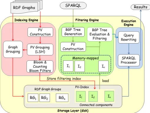
IMPLEMENTATION OF RIQ 4.1 System Architecture
RIQ consists of three distinct engines: the Indexing Engine, the Filtering Engine, and the Execution Engine (Figure 12).
The Indexing Engine is responsible for four tasks. The first task is the con-struction of Pattern Vectors from the input RDF graphs. Algorithm 1 in Chapter 3
Figure 13. Filtering Index generation in RIQ
describes the PV construction. Having transformed all RDF graphs into sets and multisets of non-negative integers (the Pattern Vectors), the Indexing Engine em-ploys Locality Sensitive Hashing (LSH) [35] to perform similarity-based grouping as described in Algorithm 3 of Chapter 3. As the individual Pattern Vectors are grouped, their corresponding RDF graphs are written to disk into separate files (one per group) where each file/group contains many RDF graphs. In addition, Bloom filters and Counting Bloom filters are generated for the grouped PVs. The BFs and CBFs are stored to disk. The collection of all BFs and CBFs for all the unions of grouped PVs comprise the filtering index called PV-Index. Figure 13 illustrates the steps and transformations.
The Filtering Engine inRIQ performs several tasks at query time. Those tasks are a part of the filtering phase of query processing where candidates of RDF graphs
which may match the query are identified. First, the Filtering Engine generates a parse tree which we call a BGP Tree out of the SPARQL query which serves as the execution plan for processing the individual BGPs. Next, the Pattern Vector for each BGP is constructed as described in Algorithm 2. This PV along with the memory-mapped PV-Index of the RDF graphs serve as the input for the BGP Tree Evaluation & Filtering task which is described in detail in Algorithm 4. Figure 14 shows the steps in testing if a group is a candidate for a query PV by using the subset operation on the corresponding vectors within the PV. The subset testing is performed using the Bloom filters and Counting Bloom filters by comparing the individual bits and counters of the data and query filters. Note that the query BFs and CBFs are constructed at query time in order for their capacity and error rate to correspond to the data BF/CBF which is being tested. If those parameters are not the same, comparing the bits and counters would be meaningless as the number of hash functions used for inserting would be different. For Bloom filters, the corresponding bits in the query BF and the data BF are checked such that BFq[i] == BFu[i]. For Counting Bloom filters, the
counters in the query CBF are compared to the corresponding counters in the data CBF such that CBFq[i]≤CBFu[i].
Finally, the Execution Engine performs the final two tasks. First, it does query rewriting by pruning the BGP Tree as described in Algorithm 6. The rewritten query can be much more efficient to process because BGPs for which there will be no matches are excluded. The rewritten queries are handed to the SPARQL Processor (an application such as Jena TDB or Virtuoso) which runs each of the rewritten queries on the corresponding candidate group indexes and outputs the results for
Figure 14. Query execution in RIQ
-,
.
'
:
.
~----"...
.
-~
-
,.
-
/.
"
-each group. Since RDF graphs do not span groups, merging of the results is trivial: they are concatenated. Note that in order for the merging to be successful, all the variables from the original SPARQL query need to be projected in the re-written, optimized queries (even if those variables are not used in the BGPs of the candidate query because they were pruned away).
4.2 Implementation
RIQ was implemented in C++ and was running as a single-threaded appli-cation. In addition to relying heavily on the C++ STL, we also used a number of external libraries. For RDF parsing of triples and quadruples, we used the highly efficient C Raptor library [20]. For SPARQL query parsing and rewriting, we used the closely-related Rasqal [21] library. We implemented our own version of LSH [38] which we had already used successfully in some of our previous papers [54, 55, 52]. For Bloom Filters and Counting Bloom Filters, we made some minor modifications to the popular Bit.ly Dablooms library [23] which allowed us to control the preci-sion and capacity of our Bloom Filters. Finally, during indexing, we used Google’s sparse hash map [3] for the efficient storing of very large in-memory hash maps of LSH buckets when building the filtering index.
We integrated three different SPARQL processors in RIQ. For RDF-3X, we used the package provided by the authors and called it using Python scripts. For Jena TDB and Virtuoso, we wrote Java applications which called their corresponding APIs.
4.3 Limitations
RIQ was designed to excel at processing queries with large, complex BGPs. As we will show in the Evaluation chapter, RIQ is able to process those queries significantly faster than both RDF-3X and Jena TDB. For queries with small, mostly star-shaped BGPs, RIQ has a competitive performance.
At the center of RIQ’s design is a successful grouping of the RDF graphs in the dataset based on their similarity using LSH where the number of groups of highly-similar RDF graphs is much smaller than the total number of graphs. If the input RDF data is very homogenous, in the worst case, RIQ will create one giant group of all the graphs. On the other hand, if the dataset contains RDF graphs which are highly dissimilar, in the worst case, RIQ will create a group for every single RDF graph. In both cases, query processing times are negatively impacted. In the first case, the one large group of graphs is equivalent to indexing the dataset with Jena TDB without using RIQ and using RIQ becomes unnecessary. The query time will be larger because it will include RIQ’s filtering time for identifying the single group. In addition, the creation of the PV-Index will significantly increase the total indexing time without providing any benefit at query time.
In the second case, where every single graph is represented by a separate group (i.e. the number of graphs is equal to the number of groups), depending on the query, RIQ is likely to identify a large number of candidates during filtering which will slow down the SPARQL processor (e.g. Jena TDB) because it will have to query a large number of small indices. The I/O is likely to increase significantly. The difference between cold and warm query times will likely decrease (the warm times
will get slower) due to the high number of page faults. In addition, both the size of the filtering index (PV-Index) and the total size of the indexed RDF data will be the largest possible because it will not be possible to take advantage of compressing graphs with common subjects, predicates or objects.
Related to the above worst case scenarios is the difficulty of figuring out the ”perfect” LSH k and l parameters (the number of hash functions used for grouping) such that the worst cases are avoided. This limitation is inherent to LSH as it is highly-dependent on the input data. Despite this limitation, LSH has been success-fully deployed over the years in a large number of applications in many domains in both research and industry [60]. We explored an alternative method for grouping of RDF graphs in RIQ. Instead of the probabilistic, estimate approach which LSH takes, we implemented a prototype of RIQ which calculated the exact Jaccard index of the PVs representing the RDF graphs in order to decide how to group them. Un-fortunately, this calculation made indexing prohibitively expensive (the indexing time grew from a few hours to a few days) without providing a significant improvement at query time. A comparison of the query times for RIQ using LSH and RIQ using Jaccard for grouping can be found in Tables 12 and 14 in the Evaluation chapter.
Another limitation which is related to the size of the groups created by LSH has to do with keeping the size of the filtering index small to minimize the I/O during filtering. The size of the PV-Index is a function of the size of the individual Bloom filters and Counting Bloom filters which represent the groups of similar RDF graphs. If we allow for the BF and CBF capacities to be equivalent to the size of the groups they represent, we risk having a very large PV-Index. On the other hand, if we set
a maximum capacity of the BFs and CBFs, we risk having too many false positives as the counters in the CBFs will start overflowing and all the bits in the BFs will be set. Two ways in which we try to minimize the I/O during filtering is first by implementing the PV-Index as a collection of memory-mapped BFs and CBFs. In addition, we choose the LSH k and l parameters, and the maximum capacity and false positive rate of the BFs and CBFs such that the size of the PV-Index is smaller than the available RAM.
While RIQ is very fast at processing queries with large, complex BGPs, it struggles with low selectivity queries which contain a match in most or all the RDF graphs. The evaluation section shows the results for two such queries (L5 and L7) which output all the graduated and undergraduate students in the LUBM dataset. The number of results for those queries is 25 and 79 million respectively. Because those queries contain a match in every single RDF graph, it is impossible for RIQ to group the graphs in such a way that the number of candidate groups is not equal to the total number of groups. This forces the SPARQL processor to query every single group in the refinement phase. One way to minimize the negative impact of such queries is to minimize the total number of groups.
CHAPTER 5 EVALUATION
In this chapter, we present the performance evaluation of RIQ. We have compared RIQ with the latest versions of three of the state of the art applications for indexing and query processing of RDF data: RDF-3X 0.3.8 [46], Apache Jena TDB 2.11.1 [18], and OpenLink Software Virtuoso OpenSource 7.10 [56]. Unlike RDF-3X, both Jena TDB and Virtuoso support RDF quads. The machine on which we conducted all the experiments was running a 64-bit Ubuntu 13.10 with Linux kernel 3.11.0 and had a 4-core Intel Xeon 2.4GHz CPU and 16GB RAM.
For Jena TDB, the default statistics-based TDB optimization was used be-cause the other settings are intended for exploring the optimizer strategy. We set the Java max heap size to 8GB (half of the available RAM). For Virtuoso, we set a number of memory-related parameters recommended by the OpenLink documenta-tion for the amount of RAM on the machine where Virtuoso is run. In particular, we set the NumberOfBuffers to 1360000 and MaxDirtyBuffers to 1000000. Futhermore, we set the MaxCheckpointRemap to 1000000. The recommended 1/4 of the Num-berOfBuffers setting caused too many re-mappings and the Virtuoso logs suggested increasing the parameter. Finally, we did not set the ShortenLongURIs parameter as we did not want to give Virtuoso an unfair advantage in the comparison with the rest of the approaches.
indexing the full BTC triples dataset which was used for running a couple of the sets of query types. After trying to index the BTC triples dataset for 6 days with Virtuoso, we gave up. However, we were able to index the BTC quad dataset for testing the multi-BGP queries.
5.1 Datasets
The evaluation was done using two datasets widely used in the Semantic Web, one synthetic and the other one real. The synthetic dataset was the Lehigh Univer-sity Benchmark (LUBM) [7]. We generated 200,004 files (and 10,000 universities) which we considered as separated RDF graphs. The dataset contained of 1.38 bil-lion triples. There were 18 unique predicates, 216,971,360 subjects, and 161,394,242 objects. There were less than 100 RDF types.
The second, real, dataset was BTC-2012 [11]. It contained 1.36 billion quads. The Billion Triple Challenge is comprised of 5 different sources of real data from different web resources: Datahub, DBpedia, Freebase, Rest, and Timbl. The total number of RDF graphs was considerably higher than LUBM: 9.59 million. Furhter-more, BTC contained a much larger number of unique predicates: 57,000. There were 183,000,000 subjects and 192,000,000 objects. In addition, BTC-2012 contained 156,000,000 literals and 296,000 different RDF types.
5.2 Queries
As explained in Chapter 2, RIQ is geared towards queries with large, complex BGPs. There were three main types of queries we evaluated: queries containing large, complex BGPs, queries with small BGPs, and finally, queries with multiple BGPs.
Table 2 shows more information about each set of queries, including the number of results and triple patterns. Appendix A lists the full text of all the SPARQL queries. The first set of queries contained many triple patterns (at least 11 and at most 22) and most of the queries contained undirected cycles. There were 3 LUBM (L1-L3) and 2 BTC large, complex BGP queries. Appendix A contains a visualization of these queries.
The second set were queries similar to the ones used in other research publi-cations: small, mostly star-shaped and some short path/chain queries. The 9 small LUBM queries (L4-L12) are variations of queries from the 14 standard LUBM bench-mark queries. Since RDF-3X does not support inferences, we used instances of the inference types from the original queries. For BTC, we used 5 small queries (B3-B7). Both the large and the small queries contained single BGPs.
For the last type, multi-BGP queries, we modified queries from the DBpedia SPARQL benchmark [44], one of the only real (non-synthetic) SPARQL benchmarks. The DBPSB is based on real queries extracted from the dbpedia.org logs. The queries contain a wide range of SPARQL grammar and are representative of real-world SPARQL usage. The subset of queries we issued used theUNION andOPTIONAL keywords which enabled us to evaluate our query rewriting optimizations. The queries contained at least 2 and at most 5 different BGPs.
5.3 Indexing
In this section, we report the size and time it took to index the two datasets along with the settings we used. Tables 3 and 4 show all the numbers.
Table 2. Queries for LUBM and BTC-2012.
Dataset Query Type # of # of # of
BGPs triple results patterns LUBM L1 large 1 18 24 L2 large 1 11 7,082 L3 large 1 22 0 L4 small 1 6 2,462 L5 small 1 1 25,205,352 L6 small 1 6 468,047 L7 small 1 1 79,163,972 L8 small 1 2 10,798,091 L9 small 1 6 440,834 L10 small 1 5 8,341 L11 small 1 4 172 L12 small 1 6 0 BTC-2012 B1 large 1 18 6 B2 large 1 20 5 B3 small 1 4 47,493 B4 small 1 6 146,012 B5 small 1 7 1,460,748 B6 small 1 5 0 B7 small 1 5 12,101,709 B8 multi-bgp 5 8 249,318 B9 multi-bgp 4 7 149,306 B10 multi-bgp 7 12 196 B11 multi-bgp 2 5 525,432
of the RDF-3X and Jena TDB LUBM indices were 77GB and 121GB respectively. The memory-mapped RIQ filter index (PV-Index) was 5.7GB. It consisted of 487 groups of Pattern Vectors of highly similar RDF graphs. It took a little over 4 hours to create the PVs. Table 3 shows the break-down of the PV-Index construction. We identify three phases in the PV-Index construction. The first one is the transformation
from original RDF data to Pattern Vectors reported above. The second one is the grouping of similar PVs by running LSH on the PVs, building a graph with PVs as vertices and connecting PVs which hashed to the same LSH buckets, and finally, calculating the connected components in the group in order to identify the individual groups of graphs. The last phase is the construction of Bloom filters and Counting Bloom filters from the groups of similar Pattern Vectors.
The LSH parameters k and l were set to 30 and 4 respectively. For BF/CBF generation, we set the false positive rate to 1% and maximum capacity (number of insertions to the filters) to 107. Note that for PVs with fewer than the above
number of elements, we used the actual size of the PV as the BF/CBF capacity. This combination achieved excellent results in terms of the size of the filter index and the accuracy with which it identified candidate groups. We show the accuracy and efficiency of RIQ in the following sections.
The BTC dataset consisted of 218GB of RDF quadruples. Due to the way it was compiled (through crawling of different Web sources), some of the data did not conform to the RDF standard and required cleaning (reformatting) or exclusion of some URIs and/or literals in order for Jena TDB and RDF-3X to parse the data correctly. We used some of the scripts and techniques used in SPLODGE [32] for cleaning the dataset. The latter’s index size was 87GB while the former was 110GB. RIQ’s filter index was 6.5GB and consisted of 526 unions of graph PVs. In this case, the LSH parameters k and l were set to 4 and 6 respectively. Because the dataset consisted of 45 times more RDF graphs, the number of LSH hash functions (k ×l) could not be very high in order for efficient indexing to occur. The CBF false positive
rate was 5% and the maximum capacity of the filters was set to 106.
Table 3. RIQ’s indexing performance: construction time Dataset Construction time (in secs)
PVs Grouping BF/CBFs Total
LUBM 15,249 22,711 3,402 41,362
BTC-2012 16,700 27,348 2,476 46,523
Table 4. RIQ’s indexing performance: settings and size Dataset # of False +ve Max. filter PV-Index
unions rate () capacity size
LUBM 487 1% 10 M 12 GB
BTC-2012 526 5% 1 M 6.5 GB
5.4 Query Processing
We conducted the query processing evaluation by collecting the wall-clock time and I/O stats (major and minor page faults) using /usr/bin/time. Two sets of experiments were done: one with cold cache where we dropped the cache using the /proc/sys/vm/drop_cacheskernel interface and one with warm cache where we ran the same query immediately preceding the warm cache experiment. Each query was run 3 times and the average was taken. In addition, we calculated the geometric mean for the three sets of queries (large, small, multi-BGP) and for all queries from
Table 5. Filtering time for RIQ on LUBM.
Query Cold cache Warm cache
Time taken Time taken (in secs) (in secs)
L1 4.03 0.15 L2 6.13 0.15 L3 4.50 0.16 L4 8.87 0.24 L5 4.44 0.10 L6 7.97 0.24 L7 5.89 0.10 L8 4.50 0.16 L9 8.22 0.25 L10 5.28 0.11 L11 5.71 0.11 L12 8.53 0.25
Table 6. Filtering time for RIQ on BTC-2012.
Query Cold cache Warm cache
Time taken Time taken (in secs) (in secs)
B1 2.30 0.11 B2 2.10 0.08 B3 2.15 0.10 B4 2.28 0.11 B5 2.14 0.11 B6 6.05 0.14 B7 2.09 0.10 B8 5.15 0.85 B9 5.12 0.78 B10 6.42 0.66 B11 6.21 0.61
a particular dataset.
We report the overall results for LUBM Table 11 and for BTC-2012 in Ta-bles 13 and 15. RIQ was able to process queries with large, complex BGPs (L1-L3) significantly faster than both RDF-3X and Jena TDB for both cold and warm cache settings. For BTC-2012, RIQ processed the large, complex queries B1 and B2 sig-nificantly faster than RDF-3X and faster than Jena TDB. These results prove that the decrease & conquer approach which RIQ takes is a better choice for processing queries with large, complex BGPs than the popular join-based processing where the individual triple patterns are first matched. All of the large, complex queries con-tained at least one undirected cycle. Appendix A shows the full text of the SPARQL queries and a visualization of the BGPs in them. RIQ was able to achieve very high precision for those queries. For LUBM queries L1-L3, out of the 487 groups of similar Pattern Vectors, RIQ identified a maximum of 16 candidate groups. For BTC queries B1 and B2, out of the 526 union groups, RIQ identified a maximum of 3 candidate groups. By discarding such a large number of groups during the filtering phase (using the PV-Index), RIQ is able to then run the queries on a much smaller portion of the dataset in the refinement phase using another tool such as Jena TDB or Virtuoso.
We report the performance evaluation of RIQ on queries with small BGPs which contain less than 8 triple patterns: queries L4-L12 and B3-B7. For LUBM, RIQ was faster than both RDF-3X and Jena TDB on four out of the nine queries for both cold and warm cache. For BTC-2012, RIQ was faster than both RDF-3X and Jena TDB in four out of the five queries for cold cache. For warm cache, RDF-3X was the winner for four out of the five queries. While RIQ’s advantage was not as strong
for small BGP queries, it was still competitive compared to the other approaches. One reason for the poorer performance on those queries is that they are generally either low-selectivity or contain graph pattern matches within most graphs. For this reason, it was impossible for RIQ to group the graphs in such a way as to minimize the number of candidates for processing during refinement time because most graphs actually contain matches for the query. However, when we compared the geometric mean of the query processing times of the three approaches, RIQ was the clear winner for both LUBM and BTC-2012 across all queries except for one case: the small BGP queries for BTC where RDF-3X won but RIQ was a close second. Tables 9 and 10 show this comparison of the geometric means for the three sets of queries for both LUBM and BTC-2012. Tables 7 and 8 show the fastest approach for processing queries over LUBM and over BTC-2012, respectively.
In the initial stages of developing RIQ, we experimented with using the Jaccard index (a.k.athe Jaccard similarity coefficient) [39] for calculating the exact similarity of Pattern Vectors instead of the probabilistic Locality Sensitive Hashing (LSH) [34] approach to similarity. Since it is impossible to exhaustively compare all Pattern Vectors to find the best match, we implemented the Jaccard index for computing the similarity of sets and multisets by using the concept of k highest cardinality sets/multisets. We pick two Pattern Vectors with the k highest cardinality of all the PVs and then we group the rest of the PVs into one of those groups. In cases of same similarity, we assign PVs to smaller groups. We also limit the size of the groups by specifying a fanout size. Tables 12 and 14 show a comparison of the query times for RIQ using the Jaccard index and RIQ using LSH for the grouping of the RDF