The Effects of Fracture Orientation and Anisotropy on Hydraulic Fracture Conductivity in the Marcellus Shale

THE EFFECTS OF FRACTURE ORIENTATION AND ANISOTROPY ON HYDRAULIC FRACTURE CONDUCTIVITY IN THE MARCELLUS SHALE

A Thesis by

MARK JOHN MCGINLEY

Submitted to the Office of Graduate and Professional Studies of Texas A&M University

in partial fulfillment of the requirements for the degree of MASTER OF SCIENCE

Chair of Committee, Ding Zhu Committee Members, A. Daniel Hill

Judith S. Chester Head of Department, A. Daniel Hill

May 2015

Major Subject: Petroleum Engineering

ii ABSTRACT

Production of hydrocarbons from low-permeability shale reservoirs has become economically feasible thanks in part to advances in horizontal drilling and hydraulic fracturing. Together, these two techniques help to create a network of highly-permeable fractures, which act as fluid conduits from the reservoir to the wellbore. The efficacy of a fracturing treatment can best be determined through fracture conductivity analysis. Fracture conductivity is defined as the product of fracture permeability and fracture width, and describes both how much and how easily fluid can flow through fractures. It is therefore directly related to well performance.

The goal of this work is to explore fracture conductivity of Marcellus shale samples fractured in both horizontal and vertical orientations. The Marcellus shale, located primarily in Pennsylvania, Ohio, West Virginia, New York, and Maryland, is the largest gas-bearing shale formation in North America, and its development has significant implications on regional economies, the northeast United States’ energy infrastructure, and the availability of petrochemical plant feedstock.

In this work, a series of experiments was conducted to determine the propped fracture conductivity of 23 different samples from Elimsport and Allenwood, Pennsylvania. Before conductivity measurements were taken, the pedigree of samples was verified through XRD analysis, elastic rock properties were measured and compared against literature values, and fracture surface contours were mapped and measured. Fracture conductivity of both horizontally and vertically-fracture samples was

iii

determined by measuring the pressure drop of nitrogen gas through a modified API conductivity cell.

Results show that fracture conductivity varies as a function of fracture orientation only when anisotropy of the rock’s mechanical properties is pronounced. It is hypothesized that the anisotropy of Young’s Modulus and Poisson’s Ratio play a significant role in fracture mechanics, and therefore in the width of hydraulically-induced fractures. Ultimately, the experiments conducted as part of this work show that fracture conductivity trends are strongly tied to both proppant concentration and the rock’s mechanical properties.

iv

DEDICATION

I would like to dedicate this work to my loving parents, Mark and Maggie, who have always stressed the importance of education and instilled in me all of my positive traits, and Desireé Johnson, who has unfalteringly supported me over the last two years. Joey Guillory, Matt Desrosiers, John White, and Clayton Madere also provided excellent mentorship and are exemplary for their support of my pursuit of education and their own teaching abilities.

Finally, I’d like to dedicate this work to Tony Loya and Monte King, who provided numerous and frequent examples of leadership that I will carry with me throughout my professional career.

v

ACKNOWLEDGEMENTS

I would like to express the sincerest gratitude to both Dr. Ding Zhu and Dr. A. Daniel Hill, who both played roles in bringing me to Texas A&M University and subsequently to their research group. From the first day, Dr. Zhu provided direction on potential research topics, approved funds for conducting important experiments that provide the basis for this thesis, permitted me to pursue external summer employment, and always had excellent insight during our weekly meetings and one-on-one

discussions.

I would also like to thank Dr. Judith Chester for serving as a committee member and supporting my work. John Maldonado and the rest of the Petroleum Engineering staff also deserve high praise; the laboratories and the Richardson Building represent a safe and clean work environment, which is a lot to ask for, considering the

circumstances. I’d also like to thank the Crisman Institute for Petroleum Research for providing XRD data for one of our Marcellus shale specimens.

Finally, I’d like to thank current and former Hydraulic Fracture Conductivity lab members Paola Perez, Ashley Knorr, Omar Enriquez Tenorio, Dante Guerra, Jesse Guerra, Zach Taylor, Kathryn Briggs, James Guzek, and Junjing Zhang, who have all either lent helping hands or acted as a sounding board for questions and issues

vi

NOMENCLATURE

A Cross-sectional flow area, L2, [ft2]

BI Brittleness Index, [-]

C’ Anisotropy ratio, [-]

Ca Areal proppant concentration, ML-2, [lb-m/ft2] cf Fracture conductivity, L2L, [md-ft]

cf0 Initial fracture conductivity, L2L, [md-ft] CfD Dimensionless fracture conductivity, [-]

dp Proppant diameter, L, [mm]

E Young’s Modulus, ML-1t-2, [MMpsi] E* Plane Strain Modulus, ML-1t-2, [MMpsi] G Energy Release Rate, MLt-1, [N/m] g Acceleration due to gravity, Lt-2, [ft/s2]

hf Sample width, L, [ft]

K Stress intensity factor, L1.5M-1t-2, [psi-ft0.5]

K’ Consistency index, [-]

k Permeability, L2, [md]

kf Fracture permeability, L2, [md] km Matrix permeability, L2, [md]

L Length of the sample, L, [ft]

vii

mp Proppant mass, M, [g]

n Number of data points, [-]

n’ Flow behavior index, [-]

p1 Inlet pressure, ML-1t-2, [psig] p2 Outlet pressure, ML-1t-2, [psig] pcell Cell pressure, ML-1t-2, [psig]

q Volumetric flow rate, L3t-1, [L/min]

R Universal gas constant, ML2t-2N-1 φ -1, [J/mol-K] RRMS Root-Mean-Square roughness, L, [in.]

r Crack tip radius, L, [ft]

T Temperature, [K]

v∞ Terminal settling velocity, L/t, [ft/s] W Mass flow rate, Mt-1, [kg/min] wd Dynamic fracture width, L, [ft]

wf Fracture width, L, [ft]

v Fluid velocity in fracture, Lt-1, [m/s]

xf Fracture half-width, L, [ft]

y Fracture surface height, L, [in]

Z Gas compressibility factor, [-]

Greek

viii

Δp Differential pressure, ML-1t-2, [psig]

λ Decline rate constant, [-]

μ Fluid viscosity, ML-1T-2T, [Pa-s]

ν Poisson’s Ratio, [-]

θ Fracture angle, [°]

ρf Fluid density, ML3, [kg/m3] ρp Proppant density, ML3, [kg/m3]

σ(r, θ) Crack tip stress in polar coordinates, LM-1t-2, [psi] σc Closure stress, LM-1t-2, [psi]

𝜙 Porosity, L3L-3, [-]

Universal tensor function, [-]

Subscripts

h Horizontal

i Iteration number

N Fracture mode designation

ix TABLE OF CONTENTS Page ABSTRACT ...ii DEDICATION ... iv ACKNOWLEDGEMENTS ... v NOMENCLATURE ... vi TABLE OF CONTENTS ... ix LIST OF FIGURES ... xi

LIST OF TABLES ... xvi

1 INTRODUCTION ... 1

1.1 Background ... 1

1.2 Literature Review ... 3

1.2.1 Marcellus Shale Overview ... 3

1.2.2 Hydraulic Fracturing in North American Shale Formations ... 11

1.2.3 Fracture Conductivity Test Method and Calculation ... 18

1.2.4 Rock Fracture Mechanics ... 21

1.3 Problem Description, Objectives, and Significance ... 27

1.4 Approach ... 29

2 EXPERIMENTAL DESIGN AND METHODOLOGY ... 32

2.1 Introduction ... 32

2.2 Shale Samples, Fluids, and Proppant ... 32

2.3 Methodology of Sample Preparation... 42

2.4 Methodology for Surface Roughness Measurement by Laser Profilometer ... 50

2.5 Methodology for Conductivity Measurement by Gaseous Nitrogen ... 53

2.6 Determination of Fracture Conductivity ... 69

2.7 Proppant Concentration Calculations ... 74

3 PROPPED SHALE FRACTURE CONDUCTIVITY ... 77

3.1 Introduction ... 77

x

3.3 Propped Fracture Conductivity of the Marcellus Shale ... 81

3.3.1 Allenwood Sample Fracture Conductivity ... 83

3.3.2 Elimsport Sample Fracture Conductivity ... 87

3.3.3 Comparison of Allenwood and Elimsport Fracture Conductivity ... 92

4 FRACTURE CONDUCTIVITY AS A FUNCTION OF ROCK MECHANICAL PROPERTIES ... 94

4.1 Introduction ... 94

4.2 Mechanical Property Anisotropy ... 102

5 CONCLUSIONS AND RECOMMENDATIONS ... 104

5.1 Conclusions ... 104

5.2 Limitations and Recommendations ... 105

REFERENCES ... 106

APPENDIX A ... 112

APPENDIX B ... 116

xi

LIST OF FIGURES

Page Fig. 1.1 – Diagram of Horizontal and Vertical Fracture Types ... 3 Fig. 1.2 – Marcellus Shale Isopach Map with Well Locations (Wang and Carr,

2013) ... 4 Fig. 1.3 – Natural Gas Production from the Marcellus Shale (U.S. Energy

Information Administration, 2014) ... 5 Fig. 1.4 – Rose Plot Showing J1 and J2 Joint Orientation (Engelder et al., 2009) ... 6 Fig. 1.5 – Stratigraphic Column of the Appalachian Basin, Including Marcellus

Shale... 8 Fig. 1.6 – The Area of Interest at the Time of Deposition, 385 Million Years Ago

(Boyce and Carr, 2009) ... 9 Fig. 1. 7 – Mineralogy of Marcellus Shale in Southwestern Pennsylvania (Boyce

and Carr, 2009) ... 10 Fig. 1.8 – Total Organic Content vs. Gas Saturation (Passey et al., 2010) ... 11 Fig. 1.9 – Settling of 40/70 Mesh Sand in Slick Water (Boyer et al., 2014) ... 15 Fig. 1.10 – Representation of Proppant Settling in Hydraulic Fracture (Boyer et

al., 2014) ... 16 Fig. 1.11 – Comparison of API RP-61 and ISO 15303 (Mod RP-61) (Palisch et

al., 2007) ... 19 Fig. 1.12 – Sample Configuration and Dimensions (Kamenov, 2013) ... 20 Fig. 1.13 – Schematic of Basic Fracture Modes: (a) Mode I, (b) Mode II, (c)

Mode III (Sun and Jin, 2012) ... 22 Fig. 1. 14 – Various Levels of Fracture Complexity (Fisher et al., 2004) ... 23 Fig. 1.15 – Interaction between Hydraulic and Natural Fractures (Dahi-Taleghani

and Olson, 2009) ... 24 Fig. 1.16 – Schematic of a Fault Zone (Johri, 2012) ... 25

xii

Fig. 1.17 – Impact of Stimulated Rock Volume on Cumulative Gas Production

(Mayerhofer et al., 2006) ... 26

Fig. 1.18 – Impact of Fracture Conductivity on Cumulative Gas Production over Time (Mayerhofer et al., 2006) ... 28

Fig. 1.19 – Workflow for Experimental Work ... 31

Fig. 2.1 – Location of Marcellus Shale Outcrops (Google Earth) ... 33

Fig. 2.2 – Research Group at Elimsport Outcrop Site ... 34

Fig. 2. 3 – Sample XRD Results ... 36

Fig. 2.4 – Inducing Mode I Fracture in Samples (Fredd et al., 2001) ... 38

Fig. 2.5 – (a) Horizontal Flow in a Horizontal Fracture, (b) Horizontal Flow in a Vertical Fracture, and (c) Vertical Flow in a Vertical Fracture ... 40

Fig. 2.6 – Depiction of Distribution of Proppant on Rough Marcellus Fracture (Zhang, 2014)... 42

Fig. 2.7 – Epoxy Cure Time as a Function of Temperature, Momentive RTV 627 (Zhang, 2014)... 44

Fig. 2.8 – Sample Preparation Mold Without Aluminum Tape (Guzek, 2014) ... 45

Fig. 2.9 – Aligning Sample Inside Sample Preparation Mold (Guzek, 2014) ... 48

Fig. 2.10 – Surface Roughness Scanning ... 52

Fig. 2.11 – Schematic of Experimental Set-up for Determination of Fracture Conductivity ... 56

Fig. 2.12 – Fully-Prepared Sample (Guzek, 2014) ... 58

Fig. 2.13 – Potentiometer Screw (Circled in Red) on Aalborg Mass Flowmeter ... 59

Fig. 2.14 – GCTS CATS Standard Screen Shots for Step 18 ... 61

Fig. 2.15 – GCTS CATS Standard Screen Shots for Step 19 ... 63

xiii

Fig. 2.17 – GCTS CATS Standard Screen Shot for Step 21 ... 65

Fig. 2.18 – Fully-Assembled Conductivity Cell ... 66

Fig. 2.19 – GCTS CATS Standard Screen Shot for Step 35 ... 68

Fig. 2.20 – GCTS CATS Standard Screen Shot for Step 36 ... 69

Fig. 2.21 – Flow Direction on Fractured Shale Sample with Proppant ... 70

Fig. 2.22 – Fracture Conductivity via Forchheimer and Darcy Equations (Zhang, 2014) ... 71

Fig. 2.23 – Computation of Fracture Conductivity via Darcy’s Equation from Experimental Results ... 73

Fig. 2.24 – PKN Fracture Geometry (Nordgren, 1972) ... 75

Fig. 3.1 – Average Fracture Conductivity and Standard Deviation with 0.013 lb/ft2 Proppant ... 84

Fig. 3.2 – Average Fracture Conductivity and Standard Deviation with 0.025 lb/ft2 Proppant ... 85

Fig. 3.3 – Summary of Allenwood Fracture Conductivity ... 86

Fig. 3.4 – Average Fracture Conductivity and Standard Deviation with 0.051 lb/ft2 Proppant ... 87

Fig. 3.5 – Average Fracture Conductivity and Standard Deviation with 0.10 lb/ft2 Proppant ... 89

Fig. 3.6 – Long-term Conductivity Results for 20/40 Resin-Coated Proppant (Jackson, 2014) ... 90

Fig. 3.7 – Summary of Elimsport Fracture Conductivity ... 91

Fig. 3.8 – Elimsport and Allenwood Fracture Conductivity with 0.051 lb/ft2 Proppant ... 92

Fig. 4.1 – Schematic of Rock Mechanical Property Anisotropy in Triaxial Testing (adapted from Cho et al., 2011) ... 95

xiv

Fig. 4.2 – Surface Contours of 04RXTH, Horizontally-Fractured Elimsport

Sample ... 96

Fig. 4.3 – Surface Contours of 10RXTV, Vertically-Fractured Elimsport Sample ... 97

Fig. 4.4 – Surface Contours of 19RNTH, Horizontally-Fractured Allenwood Sample ... 97

Fig. 4.5 – Surface Contours of 16RNTV, Vertically-Fractured Allenwood Sample ... 98

Fig. 4.6 – Fracture Schematic of Vertical (0° and 15°) and Horizontal (80° and 90°) Fractures (Tavallali and Vervoort, 2010) ... 99

Fig. 4.7 – Boryeong Shale Specimens after Failure in Uniaxial Compression Tests (Cho et al., 2011) ... 100

Fig. 4.8 – Fracture Propagation Path through Vertical and Horizontal Fractures (adapted from Liu et al., 2013) ... 101

Fig. B.1 – Fracture Conductivity vs. Closure Stress with 0.10 lb/ft2 Proppant ... 116

Fig. B.2 – Fracture Conductivity vs. Closure Stress with 0.051 lb/ft2 Proppant ... 116

Fig. B.3 – Fracture Conductivity vs. Closure Stress with 0.025 lb/ft2 Proppant ... 117

Fig. B.4 – Fracture Conductivity vs. Closure Stress with 0.013 lb/ft2 Proppant ... 117

Fig. C. 1 – Surface Contours of 03RXTH, Horizontally-Fractured Elimsport Sample ... 119

Fig. C. 2 – Surface Contours of 09RCTV, Vertically-Fractured Elimsport Sample ... 119

Fig. C. 3 – Surface Contours of 13RCTV, Vertically-Fractured Elimsport Sample ... 120

Fig. C. 4 – Surface Contours of 14RNTV, Vertically-Fractured Allenwood Sample ... 120

Fig. C.5 – Surface Contours of 15RNTV, Vertically-Fractured Allenwood Sample ... 121

Fig. C.6 – Surface Contours of 17RNTH, Horizontally-Fractured Allenwood Sample ... 121

xv

Fig. C.7 – Surface Contours of 18RNTV, Vertically-Fractured Allenwood

Sample ... 122 Fig. C.8 – Surface Contours of 20RNTH, Horizontally-Fractured Allenwood

Sample ... 122 Fig. C.9– Surface Contours of 21RNTH, Horizontally-Fractured Allenwood

Sample ... 123 Fig. C.10 – Surface Contours of 22RNTH, Horizontally-Fractured Allenwood

Sample ... 123 Fig. C.11 – Surface Contours of 23RNTV, Vertically-Fractured Allenwood

xvi

LIST OF TABLES

Page

Table 1.1 – Summary of North American Shale Play Properties (Zhang, 2014) ... 13

Table 1.2 – Simplified Fracture Treatment Schedule for Marcellus Shale ... 17

Table 2.1 – Mineral Content of Various Marcellus Shale Samples by XRD Analysis (Boyce and Carr, 2009; Lash and Engelder, 2011; Olusanmi et al., 2012; Wang and Carr, 2013) ... 37

Table 2.2 – Various Estimations of Propped Fracture Width in Shale Plays ... 74

Table 3.1 – Test Permutations of Propped Fracture Conductivity ... 78

Table 3.2 – Depiction of Tested Proppant Loading ... 80

Table 3.3 – Summary of Allenwood and Elimsport Rock Properties ... 81

Table 3.4 – Anisotropy between Horizontal and Vertical Property Values ... 82

Table 4.1 – Total Fracture Length as a Function of Sample Orientation (adapted from Tavallali and Vervoort, 2010) ... 100

Table A.1 – Conductivity Values for Samples at 0.10 lb/ft2 Proppant Loading ... 112

Table A.2 – Conductivity Values for Samples at 0.051 lb/ft2 Proppant Loading ... 113

Table A.3 – Conductivity Values for Samples at 0.025 lb/ft2 Proppant Loading ... 114

Table A.4 – Conductivity Values for Samples at 0.013 lb/ft2 Proppant Loading ... 115

Table C.1 – Individual Sample Root-Mean-Square Roughness... 118

1

1 INTRODUCTION 1.1 Background

In low-permeability formations, such as the Marcellus shale, hydraulic fracturing is used to stimulate production from an otherwise unproductive reservoir. Matrix permeability in the Marcellus shale, estimated between 1 10-6

and 0.01 md, is

insufficient for production of hydrocarbons via conventional means (Myers, 2008). To enhance production, a stimulation method known as hydraulic fracturing is utilized.

In hydraulic fracturing, a fluid carrying proppant is pumped into the formation at pressures sufficient to fracture the formation. Proppant, usually sand or spherical ceramic particles, is used to maintain a desirable fracture width in the absence of the high-pressure fracturing fluid. After the fractures’ propagation has been arrested, fracturing fluid is withdrawn from the reservoir during the flowback period. As this occurs, the formation slowly returns to its equilibrium pressure. During this process, fractures close in on proppant, and the remaining proppant acts as a barrier to fracture closure, providing sufficient fracture width for production.

The most common parameter used to describe the effectiveness of a hydraulic fracturing job is fracture conductivity. This parameter is the product of fracture width and fracture permeability; it is expressed in units of md-ft, as shown below,

... (1-1) Conductivity can also be expressed in a dimensionless form, which compares the

fracture conductivity to the formation conductivity,

2

Opinions vary on best practices for hydraulic fracturing, but in general, the fracturing fluid, proppant size, proppant type, or proppant concentration can be varied independently or in combination in order to optimize fracture conductivity. Due to various economic considerations in the Marcellus shale, including the high ratio of relatively low-value dry gas to high-value condensate or oil, fracturing design usually takes a low-cost route in the form of slickwater fluid and natural white sand proppant.

Typically, fracture conductivity of shale is measured in a laboratory setting using either outcrop or core samples from the desired formation. A rough fracture is initiated parallel to the bedding planes of the formation and then split in tension, simulating a horizontal fracture. By measuring the pressure drop of a fluid passing through the fracture face under sealed conditions, fracture conductivity can be estimated. However, this fracture conductivity measures the conductivity of a horizontal fracture, rather than that of a vertical fracture.

In the Marcellus shale, the productive interval is located between 4,000 and 8,500 feet of total vertical depth (TVD), where fractures most commonly propagate vertically due to the high overburden stress at these depths (Shelley et al., 2014). In formations exhibiting significant mechanical property anisotropy, it is conceivable that the horizontal and vertical fracture conductivities are significantly different (Chen et al., 1996). The goal of this research is to investigate the differences of horizontal and vertical fracture conductivity, particularly in the Marcellus shale, so that better estimates of field conditions can be made based on laboratory studies in order to avoid costly mistakes. A schematic of horizontal and vertical fractures is shown in Fig. 1.1. Previous

3

research has indicated a strong correlation between the absolute values of rock

mechanical properties and conductivity (Jansen, 2014); this will also be investigated as it pertains to Marcellus shale specimens.

Fig. 1.1 – Diagram of Horizontal and Vertical Fracture Types

1.2 Literature Review

1.2.1 Marcellus Shale Overview

The Marcellus shale is a primarily gas-bearing organic black shale formation that covers large swaths of Pennsylvania and extends into New York, Ohio, West Virginia, Virginia, and Maryland. Bearing up to 410 trillion cubic feet of proven gas reserves, it is posited to be the largest shale-gas formation in North America (Shelley et al., 2014).

4

Successfully extracting gas from the Marcellus shale has enormous implications on regional economies, the northeast United States’ energy infrastructure, and the availability of petrochemical plant feedstock. Due to highly repeatable and efficient drilling and completions methods, the Marcellus shale also exhibits the lowest breakeven price when compared to other North American shale plays, at a natural gas price of $3.17 per thousand cubic feet (Schweitzer and Bilgesu, 2009).

As the isopach map in Fig. 1.2 shows, the thickest sections of the Marcellus are located in northeastern Pennsylvania and at the juncture of Pennsylvania, West Virginia, and Maryland. As shown in Fig. 1.3, gas production increased exponentially in the Marcellus region from 2007 to 2015.

5

Fig. 1.3 – Natural Gas Production from the Marcellus Shale (U.S. Energy Information Administration, 2014)

Ongoing volatility of hydrocarbon commodity prices is added incentive to improve the evaluation of fracture conductivity prior to drilling, as it could significantly reduce drilling costs and improve the profitability of drilling in this region.

Two sets of natural joints trending northeast and southwest characterize the fissile, Devonian-age Marcellus shale. The so-called J1 and J2 joint sets, caused by the pressurization of organic matter during its thermal maturation and burial, can be

exploited to enhance production in horizontal wells. Fig. 1.4 below shows the presence of these faults in the Marcellus shale. Most commonly, the plane of least principal stress is roughly perpendicular to the J1 joint set. Coincidentally, the J1 joints are also more closely spaced than the J2 joints, meaning that the combined matrix and fracture

6

permeability is greater in the J1 direction (Engelder et al., 2009). Drilling wells that orthogonally intersect one of the joint sets is common practice, as it increases the well’s exposure to natural fractures and also ensures that the well is oriented perpendicular to the plane of least principle stress (Engelder et al., 2009). When undergoing a hydraulic fracture treatment, the rock fractures perpendicular to the plane of least principle stress, resulting in fractures that propagate directly away from the wellbore.

7

Like most black shales, the Marcellus has long been widely considered to be the source for an overlying conventional reservoir, but unlikely to be a productive interval in and of itself. A stratigraphic column of the Marcellus shale and surrounding formations is shown in Fig. 1.5. Wells drilled into the underlying conventional reservoir, the Oriskany sandstone, frequently experienced blowouts during its development in the mid-20th century. The natural faults of the Marcellus shale are now thought to have

contributed to these gas blowouts. Both the faultless nature of the Oriskany sandstone and the low matrix permeability of the Marcellus support the idea that a network of natural fractures in the Marcellus shale contributed significantly to the presence of free, high-pressure gas in the Marcellus interval (Engelder et al., 2009).

The Middle Devonian Appalachian Basin sequence of shale and limestone represents, “the initiation of the Devonian-Mississippian anoxic event in the central Appalachian basin” (Boyce and Carr, 2009). During its deposition roughly 385 million years ago, the Appalachian Basin was a marine environment surrounded by the

Cincinnati Arch to its west, the Rheic Ocean to the south, and the Acadian Mountains to the east. Fig. 1.6 shows the current Marcellus shale region outlined in red, as well as the paleogeographic features described above. Based on total organic content and gamma ray values, the Middle Devonian units appear to have been deposited in environments with varying availability of oxygen. The Marcellus and Harrell shales, for example, exhibit extremely high gamma ray values and are therefore likely to have been deposited in an anoxic environment, where bacteria that consume organic material could not survive. Units such as the Mahantango, which has a characteristic gamma ray signature

8

lower than that of the Marcellus, was likely deposited in a suboxic environment. Units such as the Tully and Onondaga limestone, which are devoid of significant gamma ray signatures, are thought to have been laid down in an environment with sufficient oxygen for decomposition of organic material by bacteria (Boyce and Carr, 2009).

9

Fig. 1.6 – The Area of Interest at the Time of Deposition, 385 Million Years Ago (Boyce and Carr, 2009)

The Marcellus shale is identified in cores as possessing a volumetric concentration of quartz up to 70% and a clay content of roughly 25%. The total thickness of the

Marcellus ranges from 50-200 feet and total organic content ranges from 3-12% (Shelley et al., 2008). For Boyce and Carr’s study, 36 cores underwent x-ray diffraction (XRD) to determine mineralogy. Those results are summarized in Fig. 1.7.

10

Fig. 1. 7 – Mineralogy of Marcellus Shale in Southwestern Pennsylvania (Boyce and Carr, 2009)

Total organic content is important because it is usually strongly correlated to the gas saturation in unconventional source rocks (Passey et al., 2010), as demonstrated in Fig. 1.8. The results in Fig. 1.8 show the correlation between total organic content and gas saturation values for dozens of shale-gas formations worldwide.

11

Fig. 1.8 – Total Organic Content vs. Gas Saturation (Passey et al., 2010)

1.2.2 Hydraulic Fracturing in North American Shale Formations

In 1947, the first successful hydraulic fracturing treatment was executed in the Hugoton gas field in Kansas by Stanolind Oil. In this first experiment, natural river sand was carried into the formation using napalm (in great surplus in the post-World War II environment) as the fracturing fluid. After injecting this mixture, the napalm gel was broken down using a gel-breaker solution and the well was put online. In this first study comprising several wells, returns were increased by up to 1,000% as compared to pre-fractured rates (Clark, 1949). In the years since this first well was “frac-ed”, engineers and researchers have sought to improve the process in many ways including the use of foams, microseismic data, manufactured proppant, and boutique fracturing fluids.

12

There are a number of operators in the Marcellus shale, and the variety of operational philosophies and its 90,000 square mile expanse makes it difficult to typify one stereotypical wellbore and fracture treatment design (Mayerhofer et al., 2011). Wells in the Marcellus are commonly completed at a depth between 4,000-8,000 feet TVD, with laterals ranging from 2,000-7,000 feet in length. Due largely to

environmental concerns, relatively few wells in the Marcellus are drilled using oil-based muds as compared to other unconventional plays such as the Haynesville shale. In 225 analyzed horizontal wells in the Marcellus, 36% used water-based muds, and the other 64% used synthetic-based mud (Guo et al., 2012).

Since the Marcellus produces almost exclusively dry gas and condensate, fracture conductivity is not as critical in this formation as in those bearing high-viscosity fluids. Low-cost drilling, completion, and production methods are popular in the Marcellus as a result of the prevalence of low-viscosity gas and its lower relative value. Natural white sand is the most common proppant utilized in fracture treatments, with 40/70 mesh sand being the most common variety. Fracture treatment designs are always changing, but approximately 40% of the sand used in horizontal Marcellus wells is 40/70 mesh sand, with the balance being 80/100 and 20/40 mesh sand (Houston et al., 2009; Mayerhofer et al., 2011; Shelley et al. 2014). Water with a small amount of friction reducer, known as slickwater, is the most common fracturing fluid (Shelley et al., 2014). In wells analyzed by Mayerhofer et al. (2011), seven fracture stages were used, and each fracture stage used five perforation clusters spaced two feet in length each over a span of 200 feet per

13

stage. Table 1.1 summarizes production information for the Marcellus and other prominent North American shale plays.

Table 1.1 – Summary of North American Shale Play Properties (Zhang, 2014)

Properties Marcellus Eagle Ford Fayetteville Barnett True Vertical Depth

(ft)

4,000-8,000 5,000-14,000

1,500-6,500 6,000-8,500

Closure stress gradient (psi/ft)

0.67-0.76 0.7-0.95 0.59-0.7 0.61-0.73

Effective closure stress (psi/ft) 2,500-6,000 2,000-8,000 1,000-5,000 3,000-5,500 Dominant hydrocarbon Gas, condensate Oil, condensate Gas Gas

Fracture Design Water frac, foam

Gelled frac, hybrid, high-way

Water frac Water frac

Proppant size (mesh) 100, 40/70, 30/50 40/70, 30/50, 20/40 100,30/70 100, 40/70, 30/50 Maximum proppant concentration (ppg) 2.5 4 2 3.5 Average concentration (ppg) 1.2 1.2 0.6 0.6

It is important to note here that fracture treatments are not static. Proppant sizes, fluid composition, and proppant concentration are all traditionally changed throughout the fracturing process. Initially, a small proppant size, such as 100 mesh, is used to prop

14

open the fracture tip, which exhibits the smallest fracture aperture. In addition to being able to reach the fracture tips, smaller proppant has several other benefits over large proppant. It is more readily suspended in a colloid as a result of its larger surface-area-to-volume ratio, and is therefore more likely to provide even coverage throughout the vertical extent of the fracture. Slickwater fluids are particularly susceptible to proppant settling, with Boyer et al. (2014) showing that at 5,000 psi, only 8.3% of 40/70 mesh natural white sand was suspended above the proppant settling line. Settling of 40/70 mesh proppant from this study is shown in Fig. 1.9. Terminal settling velocity, v∞,

derived by Brannon and Pearson (2007) is dependent on proppant diameter and given by,

[( )

]

⁄

15

Fig. 1.9 – Settling of 40/70 Mesh Sand in Slick Water (Boyer et al., 2014)

The distribution of proppant within the fracture is also dependent on fracture geometry and the composition of the fracturing fluid. A graphical representation of proppant settling within a fracture is shown in Fig. 1.10. In order for proppant to reach a

particular region of the fracture, its entire flow path must have an aperture greater than the proppant diameter. As a result, a continuous fracture may exhibit regions with no proppant, or a partial monolayer, full monolayer, or multiple layers of proppant.

16

Fig. 1.10 – Representation of Proppant Settling in Hydraulic Fracture (Boyer et al., 2014)

The final advantage for small proppant is that it is less susceptible to screen-out. Screen-out refers to the condition wherein pumping pressure exceeds the pumping equipment’s maximum allowable working pressure as a result of the proppant pack blocking the fracture flow path. This condition has three primary causes: large proppant that becomes wedged in the fracture, fracturing fluid leak-off, and high proppant

concentration. Once screen-out has been detected, fracturing at that stage must cease, so delaying screen-out as long as possible is desirable. Operators and field service

providers typically work together to determine an appropriate pumping pressure, as well as the schedule for increasing proppant size and proppant concentration so as to create

17

the most extensive fracture network and avoid premature screen-out. A simplified fracture treatment for one stage in the Marcellus may look like that shown in Table 1.2.

Table 1.2 – Simplified Fracture Treatment Schedule for Marcellus Shale

Stage Fluid Volume (gal) Proppant Concentration (ppg) Proppant Size Pad 8,000 0 - 1 4,000 0.5 100% 100 mesh 2 4,000 1.0 50% 100 mesh, 50% 40/70 mesh 3 4,000 1.5 100% 40/70 mesh 4 3,000 2.0 50% 40/70 mesh, 50% 30/50 mesh 5 1,500 2.5 100% 30/50 mesh Flush 6,000 0 -

Since the aperture of a fracture typically decreases as the distance to the wellbore increases, larger proppant is typically called for in the final stages of a fracturing

treatment in order to maximize fracture width.

18

1.2.3 Fracture Conductivity Test Method and Calculation

The standard long-term conductivity test method for determining proppant pack conductivity is outlined by ISO 13503-5:2006. This method, traditionally used to evaluate the conductivity of proppant, calls for the use of smooth saw-cut Ohio

sandstone and a 2% KCl solution. Conductivity is measured at various pressures, all of which must be maintained for 50 hours during conductivity measurement. These tests are extremely time-consuming and resource-intense. The test is designed to eliminate as many variables as possible in order to provide fair comparisons of proppant. The 2% KCl solution used as the stand-in for fracturing fluid also causes irreversible damage to the sample and proppant, rendering each sample usable only once. This test is

essentially a modified version of the API’s own short-term conductivity test, API RP-61. Fig. 1.11 shows that the ISO standard’s test procedure can result in up to an 85%

19

Fig. 1.11 – Comparison of API RP-61 and ISO 15303 (Mod RP-61) (Palisch et al., 2007)

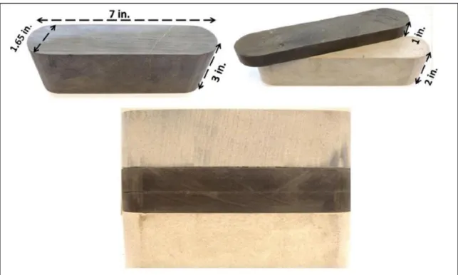
Since these standards are not intended to provide an accurate representation of fracture conductivity and are both extremely time-consuming and expensive to run, determination of fracture conductivity for this work was executed via alternate means. First, in order to maintain sample integrity for multiple tests, the 2% KCl solution was replaced with dry nitrogen gas, which is inert in the testing environment (Zhang et al., 2014). Second, since the goal of these tests is to evaluate fracture conductivity, the Ohio sandstone was replaced with Marcellus shale samples, which were obtained from two different outcrop locations. The overall sample dimensions are consistent with API sample dimensions as shown in Fig. 1.12.

20

Fig. 1.12 – Sample Configuration and Dimensions (Kamenov, 2013)

To simplify the experimental procedure, proppant was manually placed on the fracture face and then inserted into the modified conductivity cell. Dynamic proppant placement has been implemented by others (Awoleke et al., 2012; Zhang et al., 2014) in order to more realistically simulate proppant transport from the wellbore to the fracture. In this setup, a proppant and fracturing fluid slurry is pumped into the fracture using positive displacement pumps. Once the pumps are shut down, the proppant remains in the fracture, and nitrogen gas is passed through the fracture to simulate the onset of production.

Several methods for calculation of propped fracture conductivity have been proposed. Darin and Huitt (1960) used laboratory measurements to demonstrate that a

21

modified version of the Kozeny-Carman relationship could be used to describe fluid flow through a proppant partial monolayer. They also showed that a proppant partial monolayer can exhibit higher conductivity (sometimes by an order of magnitude) than multiple layers of the same proppant. More recent proposals for calculation of propped fracture conductivity include those by Gao et al. (2012), who suggest that modeling the effects of proppant embedment, deformation, elasticity, and size can improve analysis of either monolayer or multilayer conductivity analysis.

1.2.4 Rock Fracture Mechanics

Of critical importance to this research is to understand how rocks fracture in realistic downhole scenarios. There are three modes of fracture opening. A Mode I fracture is an opening fracture induced by a tensile stress. A Mode II fracture is a sliding fracture, induced by a shear stress that acts in the direction parallel to the fracture. A Mode III fracture is a tearing fracture, which is induced by a shear stress perpendicular to the plane of the fracture. Fig. 1.13 is a schematic of all three fracture modes.

22

Fig. 1.13 – Schematic of Basic Fracture Modes: (a) Mode I, (b) Mode II, (c) Mode III (Sun and Jin, 2012)

The stress at the tip of an ideal fracture can be described as, ( )

√ ... (1-4)

where KN is the stress intensity factor for one of the three fracture modes. The stress

intensity factor, KN, is a term that can be determined numerically, analytically, or

experimentally. However, as demonstrated by Shylapobersky and Chudnovsky (1992), hydraulic fractures rarely display the same net fracture pressure as would be predicted by Equation 1-4.

The propagation of fractures is also of great interest for this work. Hydraulic fractures are usually thought of as planar, bi-wing, and vertically-oriented, which can be a gross oversimplification. Seminal work by Cinco-Ley and Samaniego (1981) that assumed the predominance of simple, planar fractures also showed that dimensionless fracture conductivity has an optimal value beyond which additional returns are minimal. Diagnostic tools such as microseismic analysis show that multi-stranded fractures are found in many different formation types, including shale (Dahi-Taleghani and Olson,

23

2009). Fisher et al. (2004) arrived at a similar conclusion via microseismic data from the Barnett shale, and their findings are shown in Fig. 1.14.

Fig. 1. 14 – Various Levels of Fracture Complexity (Fisher et al., 2004)

The presence of natural fractures can also lead to increased fracture complexity. As a hydraulic fracture propagates through the formation, it can encounter existing natural fractures, microcracks from previous hydraulic fracturing stages, or otherwise weakened zones (thin beds of weaker rock, depositional discontinuities, etc.). When dealing with a formation with natural fractures such as the Marcellus shale, there are three possible scenarios for interaction of hydraulic and natural fractures, as depicted in Fig. 1.15. In (a), the hydraulic fracture bypasses the natural fracture. In (b), the hydraulic fracture is re-routed exclusively into the natural fracture, and in (c), the hydraulic fracture crosses the natural fracture and crack tips propagate in both the natural fracture and the

24

Fig. 1.15 – Interaction between Hydraulic and Natural Fractures (Dahi-Taleghani and Olson, 2009)

The idea that fractures frequently diverge from a linear path is also verifiable in the larger context of the whole formation. Frequently sandwiching faults are damage zones, which greatly add to the overall fracture network. Damage zones are highly fractured; these zones are the result of a highly-stressed fault leading to fractures outside of the original fault plane. Additionally, these damage zones often have much higher permeability than the fault core itself (Johri, 2012). The damage zones around a fault, typically the adjacent 60-100 meters to either side, are much greater in size than the fault core itself, which is usually less than 50 centimeters wide. A diagram of a fault and its associated damage zone is shown in Fig. 1.16.

25

Fig. 1.16 – Schematic of a Fault Zone (Johri, 2012)

Although complex fractures do not always result in a larger stimulated rock volume than a planar, bi-wing fracture, fractures that take advantage of natural

weaknesses in the rock will experience a lower fracturing fluid pressure drop and allow the fracturing fluid to propagate further into the formation, so it stands to reason that complex fractures generally result in a larger stimulated rock volume. The importance of maximizing stimulated rock volume is shown in Fig 1.17, which shows that a threefold increase in stimulated rock volume results in three times greater production over a fifteen-year well life.

26

Fig. 1.17 – Impact of Stimulated Rock Volume on Cumulative Gas Production (Mayerhofer et al., 2006)

The direction of crack propagation in a fracture is a function of the crack’s energy release rate, G,

( )

... (1-5) where E* can be described as,

( ) ... (1-6)

and KI and KII are the stress intensity factors for Mode I and Mode II fractures.

If G is greater than the critical energy release rate, Gc, then the crack will propagate

critically. The crack propagates in the direction that yields the highest energy release rate, and in anisotropic rock, this may result in a highly complex fracture that exhibits higher fracture conductivity than a planar fracture. Herein lies the importance of

27

that result in anisotropic elastic rock properties. Cracks can also grow in a sub-critical state (G < Gc), but for this to occur, the host material must be weakened, generally via

chemical means (Dahi-Taleghani and Olson, 2009). The maximum energy release rate can be expressed as,

̅ ̅ ... (1-7)

Where,

̅ ( ) [ ( ) ] ... (1-8)

And,

̅ ( ) [ ( )] ... (1-9) In these expressions, θ0= 0 describes a state where the fracture propagates in a straight

direction, as expected in Mode I fracturing, and ̅ is the energy release rate in a particular orientation.

1.3 Problem Description, Objectives, and Significance

Fracture conductivity in horizontally-drilled, hydraulically-fractured wells is of great importance. As shown in Fig. 1.18, a small change in fracture conductivity greatly impacts a well’s cumulative production.

28

Fig. 1.18 – Impact of Fracture Conductivity on Cumulative Gas Production over Time (Mayerhofer et al., 2006)

For the above figure, each curve represents a reservoir with the same stimulated rock volume, so production increases are due solely to the increased fracture conductivity. An increase from 0.5 md-ft to 5 md-ft results in a four-fold increase in production over the displayed five years, and increasing conductivity to 50 md-ft improves production by more than a factor of seven.

Many previous studies have established that fracture conductivity is a parameter with significant leverage on cumulative production. Some of these studies have focused on sandstone reservoirs, determining conductivity of proppant packs, or have used concentrations of proppant that are not realistic for shale formations. The work here focuses on determining fracture conductivity at reasonable proppant concentrations for the Marcellus shale, which has not been extensively studied.

29

The disparity in fracture conductivity between horizontal and vertical fractures is also poorly understood. This gap in knowledge applies to all formations, the Marcellus shale included. Rock properties that may depend on orientation, such as Young’s Modulus and Poisson’s Ratio, are known to impact fracture characteristics. It is conceivable that the anisotropy of rock properties would be manifested as differences between horizontal and vertical fracture conductivity.

The objective of this work is to quantify how differences in rock properties impact fracture conductivity, if at all. Typically, conductivity testing for fractures utilizes samples with horizontal fractures. However, the depths at which most North American shale plays are being completed would suggest that the bulk of hydraulic fracturing results in vertical fractures. Therefore, this work presents a comparison of horizontal and vertical fracture conductivity.

1.4 Approach

Procedures for the experimental approach to this work are detailed below: (1) Collect Marcellus shale samples from two sites in central Pennsylvania. (2) Ascertain the samples’ mineralogy using X-Ray Diffraction, and compare

these results with the mineralogy of other known Marcellus samples. This verifies the pedigree of the rock and ensures that the conductivity test results are representative of what might be seen in a typical Marcellus well.

(3) Divide the samples into two groups: those to be fractured horizontally, and those to be fractured vertically. Horizontal fractures are commonly used for

30

laboratory testing for several reasons. First, fracturing shale samples parallel to the bedding planes is significantly easier than fracturing through multiple bedding planes. Secondly, horizontally-fractured samples are far less likely to fail during the fracturing process, saving both time and resources. Finally, the Cooke conductivity cell used for conductivity experiments is a device that requires communication between the fracture and a small pressure port, so a vertical fracture, which is generally much rougher, may not align with the pressure port, thereby rendering a viable experiment impossible. The current industry standard is to test horizontal fracture conductivity, so the results of horizontal fracture conductivity tests are comparable to those conducted by operators. Despite the difficulty of inducing a vertically-oriented fracture in Marcellus shale samples, vertical fractures are the prevailing fracture

orientation in this and most other North American shale formations. (4) Determine Poisson’s Ratio and Young’s Modulus for both sets of samples in

both the horizontal and vertical orientation

(5) Scan fracture surfaces using a laser profilometer to determine fracture root-mean-square roughness. This step is to be repeated after each conductivity test in order to obtain information about deformation of the fracture after testing.

(6) Run conductivity tests using 40/70 white mesh sand proppant at

concentrations representing 0.16 pounds of proppant per gallon of fluid (ppg), 0.33 ppg, 0.65 ppg, and 1.3 ppg.

31

(7) Compare and contrast results of horizontally- and vertically-fractured samples.

The flowchart in Fig. 1.19 demonstrates the experimental workflow described above.

Fig. 1.19 – Workflow for Experimental Work Collect Samples

Verify Mineralogy Test Elastic Rock Properties

Fracture Rocks (Horizontally or Vertically) Scan Fracture Surfaces

Test Fracture Conductivity Analyze Results

32

2 EXPERIMENTAL DESIGN AND METHODOLOGY 2.1 Introduction

Conductivity experiments have traditionally aimed to benchmark the quality of a particular proppant or to illuminate the economic potential of exploration acreage. Fracture conductivity results can be further used to history match data from analogous wells or to predict a well’s future performance.

The goal for both of these types of tests is to produce reproducible and realistic results. Appropriate equipment calibration schedules, strict adherence to procedures, and reusing samples whenever possible helps to ensure that results are reproducible. Realistic results can be obtained by matching reservoir conditions such as closure stress, fracture orientation, fracture mode, and operating conditions such as proppant type and concentration. The latter requires that the sample be a close facsimile of the reservoir in its downhole state.

This chapter describes the selection of materials, preparation of equipment and samples, and provides procedures for all of the work undertaken. Means of limiting errors and troubleshooting are also described herein.

2.2 Shale Samples, Fluids, and Proppant

Shale samples for this research were obtained from two outcrop locations shown in Fig. 2.1. The Elimsport location was previously used by a leaseholder in the

Marcellus to excavate shale samples for large-block triaxial fracture testing. The material surrounding the original large block test samples had also been excavated and

33

deposited in large debris piles. These piles provided plenty of rocks from which 13 suitable conductivity samples were obtained.

Fig. 2.1 – Location of Marcellus Shale Outcrops (Google Earth)

As shown in the background of Fig. 2.2, the outcrop samples were exposed to the elements, and most of the material on the surface of the debris pile was both friable and soft, most likely as a result of water imbibition by the shale. After selecting suitable samples that appeared undamaged by weathering, they were wrapped in polyethylene and bubble wrap to lessen the effects of humidity and minimize shipping damage.

34

Fig. 2.2 – Research Group at Elimsport Outcrop Site

The second set of 10 samples was obtained from an excavation site in Allenwood, Pennsylvania. This site is approximately 10 miles from the Elimsport location, and samples were purchased from a third party. The parent rock for these samples was excavated from 20 feet underground, isolated from the potentially harsh effects of weathering.

Mineralogy of both sample sets was then assessed using X-Ray Diffraction (XRD). The machine and software used to analyze these two samples is only capable of qualitative, rather than quantitative, analysis. The results of the mineralogical testing are shown in Fig. 2.3, and highlight only the presence of minerals, not the volumetric

35

based on qualitative analysis, but quantitative analysis was required to determine that the concentrations of minerals is representative of the Marcellus shale. Third-party

quantitative XRD analysis of an Allenwood sample was performed, which revealed that the mineral content of these samples is in line with established literature values.

Although the exact volumetric concentration of minerals in the Elimsport samples remains unknown, the qualitative results indicating that the Elimsport and Allenwood samples are very similar can be used to draw the conclusion that the Elimsport samples are also representative of the Marcellus shale. Table 2.1 compares these results to examples of Marcellus shale from other literature.

Having verified that the collected samples have similar mineral volumetric concentrations to the samples from literature, the samples were cut to fit into the modified API conductivity cell. In order to preserve sample material, a thin (1.5-2 inches thick) shale sample was cut, and then backed with Berea sandstone to make up the remainder of the required six-inch sample thickness as depicted previously in Fig. 1.12.

36

Fig. 2. 3 – Sample XRD Results

E li m sp or t Allenw ood

37

Table 2.1 – Mineral Content of Various Marcellus Shale Samples by XRD Analysis (Boyce and Carr, 2009; Lash and Engelder, 2011; Olusanmi and Sonnenberg, 2013;

Wang and Carr, 2013)

Sample Quartz % Calcite % Dolomite % Pyrite % Clay %

Allenwood 41 12 1 12 25

Boyce and Carr 67.4 0.3 0 5.2 27.2

Lash and Engelder, Sample A

48 4 0 15 33

Lash and Engelder, Sample B 58 19 0 4 19 Olusanmi and Sonnenberg, Sample A 50 4 2 8 36 Olusanmi and Sonnenberg, Sample B 48 41 0 0 11 Olusanmi and Sonnenberg, Sample C 35 5 2 10 48

Wang and Carr, Sample A

62.04 8.25 0 0 29.71

Wang and Carr, Sample B

50.12 28.96 0 0 20.93

Wang and Carr, Sample C

38

The standard API conductivity test for benchmarking proppant performance uses rough-sawn sandstone to model fractures. This method is well-suited for comparing proppant, but for this research, natural fractures were required to best represent operational conditions. Using a masonry rock splitter, fractures were induced in the samples in a manner shown in Fig. 2.4.

Fig. 2.4 – Inducing Mode I Fracture in Samples (Fredd et al., 2001)

The compressive forces from these blades are translated as tensile forces at the fracture initiation site, resulting in a Mode I fracture. As a goal of this work was to compare horizontal and vertical fracture conductivity, half of the samples were fractured in a manner that resulted in horizontally-oriented fractures, and the other half were fractured to create vertically-oriented fractures.

39

To approximate horizontal fractures, samples were broken parallel to the bedding planes. Although the bedding planes may have a non-zero dip angle at formation depths, the dip angle is assumed to be low enough to make this a valid approximation. That said, fractures in formations such as the Marcellus do not usually propagate horizontally because of the large overburden pressure at depth. However, the current literature on the subject of propped fracture conductivity has used horizontally-fractured samples for discussion. Operators who test fracture conductivity also generate samples with this fracture orientation, meaning that horizontally-fractured samples remain the best way to compare results from this work to those from previous studies or operator data.

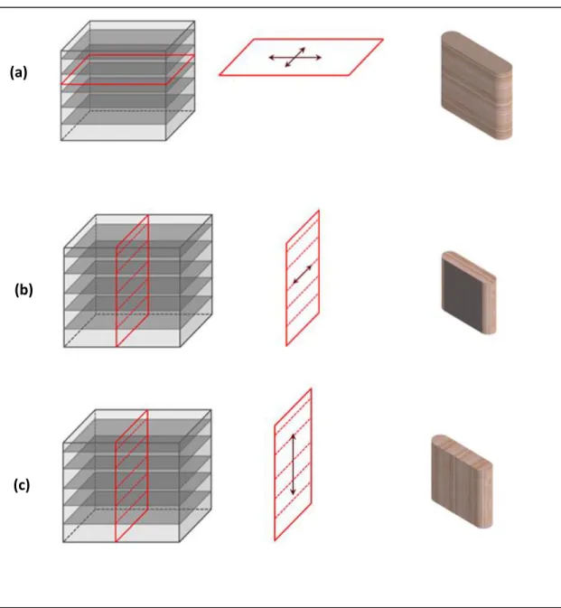
Vertically-fractured samples were cleaved perpendicular to the bedding planes; this more closely approximates flow through a vertical fracture. As depicted in Fig. 2.5, there are three basic flow paths within the two possible fracture orientations that could impact fracture conductivity. This study uses samples fractured in the first and third configurations. Zhang (2014) asserted that fracture conductivity is independent of fracture orientation, as several properties that dictate fracture conductivity such as mineralogy, interaction with water, and proppant distribution are not directional. However, properties such as Young’s Modulus and Poisson’s Ratio, both of which are related to crack propagation direction, are usually anisotropic in layered materials such as shale.

40

Fig. 2.5 – (a) Horizontal Flow in a Horizontal Fracture, (b) Horizontal Flow in a Vertical Fracture, and (c) Vertical Flow in a Vertical Fracture

In many cases, fracturing resulted in fracture infill material that had spalled from the surface. This infill appeared to be anhydrite or shale, which has been noted in other literature (Zhang, 2014). In-situ spalled material acts as a low permeability proppant, helping to increase fracture width (Kamenov, 2013). Care was taken to ensure that infill

(b)

(c) (a)

41

remained as close to its original position as possible by cutting rocks in such a manner as to minimize vibration and material loss. Following the sample fracturing process, the samples were taped for shipment.

While many fracturing fluids are water-based, shale is sensitive to swelling by means of water imbibition, and this would destroy the samples at high closure stress, cause significant changes in the fracture’s surface characteristics, or irreversibly change elastic properties essential to fracture conductivity. Similar irreversible changes also occur with use of synthetic fracturing fluids. As sample availability was limited, room-temperature nitrogen gas was used as the fluid for all conductivity tests.

40/70 mesh natural white sand was used as the proppant for these experiments and was sourced from an open-pit mine in Wisconsin operated by Badger Mining Corporation. This proppant was manufactured in compliance with ISO 13503-2:2006. Because proppant was placed manually, as opposed to being pumped into location as slurry, proppant tended to accumulate on the sample’s troughs and plateaus as depicted in Fig. 2.6.

42

Fig. 2.6 – Depiction of Distribution of Proppant on Rough Marcellus Fracture (Zhang, 2014)

2.3 Methodology of Sample Preparation

Significant preparation is required to make suitable samples for conductivity testing. This section attempts to describe a procedure to consistently create functioning samples. The following supplies are required for this procedure:

 Silicone potting compound (Momentive RTV 627)  Silicone release spray (Molykote 316)

 Rubber adhesive primer (Momentive SS 4155)  Two-part epoxy glue

 Sample mold (clamshell halves, baseplate, and screws)  Aluminum tape

 Personal attire: lab coat, long pants, close-toed shoes, protective eyewear, and latex or nitrile gloves

43  Box cutter/utility knife

 Permanent marker

 Contractor’s masking tape  Steel wool

 Tongue depressor

 Large weights or 24-in bar clamps  Acetone  Allen wrenches  Scoopula  Putty knife  Foam brush  250 gram scale  Tabletop sample oven

The silicone potting compound described, Momentive RTV 627, has a cure time curve shown in Fig. 2.7. For this work, samples were cured for a period of three hours at 160 °F. Through trial-and-error, this was found to be the temperature that optimized the cured epoxy’s strength and malleability. Curing at higher temperatures results in a sample with a more brittle epoxy coating; this is undesirable, as brittle epoxy tends to tear and delaminate from the substrate under the compressive loading of the conductivity tests, making reapplication of epoxy necessary in order to repeat testing on the same specimen.

44

Fig. 2.7 – Epoxy Cure Time as a Function of Temperature, Momentive RTV 627 (Zhang, 2014)

The clamshell-type sample mold is 0.003 inches wider than the modified API conductivity cell used in fracture conductivity testing. This makes for a slight

interference fit, ensuring that leakage is unlikely, even at high pressures. The mold is 0.15 inches wider than the bare rock specimens, meaning that uniformly centered in the mold, the epoxy coating is 0.075 inches wide around the entire sample. The sample mold is shown in Fig. 2.8.

45

Fig. 2.8 – Sample Preparation Mold Without Aluminum Tape (Guzek, 2014)

The procedure for preparing a Marcellus shale sample is as follows:

(1) Don protective eyewear, lab coat, long pants, closed-toe shoes and nitrile gloves

(2) Open package containing sandstone backing and shale sample from Kocurek Industries using box cutter

Note: The package should stay sealed until a sample is ready to be prepared, as moisture can affect the sample’s physical characteristics

(3) Place paper towel under work area to prevent glue from bonding to work surface

46

Note: Kocurek Industries has induced a fracture on the shale sample, so it is extremely important to avoid dropping the sample or damaging it in any way. Once the tape has been removed, use caution to keep both halves of shale sample together

(5) With permanent marker, label sandstone with sample designation and flow direction

Note: Sandstone should have the following information: Left/Right, sandstone thickness in inches, and sample name

Note: Sample name has the following format: first two digits are sample number (01-99), followed by parent rock name (Rock A = RA, unknown parent = RX), followed by mold height (tall=T, short =S), followed by fracture direction (H=horizontal, V=vertical)

(6) Re-tape shale sample around the fracture circumference using masking tape. Coarsen tape surface with steel wool to improve adhesion of rubber epoxy, using steel wool to remove tape’s non-stick coating

(7) Prepare two-part glue epoxy using provided glue basin and tongue depressor Note: Total required amount should not exceed 1-2 teaspoons

(8) Apply thin, even layer of glue to sandstone with tongue depressor, and attach shale sample

(9) Apply thin, even layer of glue to other sandstone piece, and place on top of shale sample

47

(10) Apply weights or bar clamps to complete sample, wiping away excess glue from sample with paper towel

Note: Applying weight or bar clamp pressure may cause sample misalignment. Do not leave sample unattended until sample and sandstone surfaces are flush with each other

(11) Using paper towel, wipe off the glue basin and tongue depressor so that they may be used again

(12) Allow glue to dry and cure for 30 minutes at minimum (13) Use acetone to clean sample mold surfaces

Note: If mold has been modified with aluminum tape (used to reduce the inner cavity dimensions), be sure to inspect mold for creases or wrinkles. If aluminum tape is excessively worn, it must be replaced

Note: To replace aluminum tape (only if required), remove old tape, apply acetone to bare surface, re-apply tape, and cut to size of mold with box cutter

(14) Place mold halves and base in fume hood, and turn on fume hood vent (15) Apply three coats of silicone release spray to all interior surfaces of mold,

waiting five minutes between each application

(16) Apply a small dab of rubber primer to foam brush over aluminum pan in fume hood, and then brush onto conductivity core sample (both shale and sandstone portions)

48

Note: Sample requires three coats of primer. Wait until white color develops on drying primer before applying subsequent coat (usually 10-20 minutes) (17) Remove mold baseplate and one half of clamshell from fume hood, and place

on flat, clean surface

(18) Screw baseplate onto one half of the clamshell using two short screws and Allen wrench

(19) Turn over baseplate and clamshell assembly, and carefully place sample inside the mold

Note: Visually align the vertical edges of the sample with the mold, making sure both edges are evenly spaced from the mold. See Fig. 2.9.

49

(20) Attach the second half of the clamshell to the baseplate, using two short screws and Allen wrench

(21) Secure two halves of the clamshell to each other using four long screws and Allen wrench

(22) Visually inspect the assembly from top view. The sample should be spaced evenly from all mold surfaces

(23) Place plastic cup on 250 gram scale, and tare scale to account for weight of cup

(24) Remove cup from scale, placing on flat surface covered with paper towel (25) Using hand-pump bottles, dispense 110 g of white epoxy compound into

12-oz cup

Note: Depress hand-pump 21 times, then add remaining amount with cup on the scale

(26) Repeat step 25 with the black epoxy component

(27) Using scoopula, stir the epoxy together so that it is an even gray color, with no areas of isolated black or white

Note: Use scoopula to make sure edges and bottom of cup are well-mixed Note: Once mixed, quickly but diligently complete sample preparation, as

curing begins immediately and epoxy begins to congeal within 20-30 minutes

50

(28) Slowly pour epoxy out of cup directly onto top surface of sample, and allow to flow over the sample and down the annulus between the sample and mold wall

Note: Overflow should ideally occur on the long edge of the sample, and preferably at just one location initially

Note: Ensure that the overflow occurs at a slow rate. The goal is to always maintain a gap between the flowing epoxy and mold interior’s top surface Note: As a rule of thumb, the pouring process should take 10-20 minutes (29) Using putty knife, wipe off epoxy from top of sample to ensure that label can

be read

(30) Carefully move sample to oven, and place in oven at heat level 3.5 (160 °F) for approximately three hours

(31) Remove sample from oven using thick leather gloves, and allow to cool for two or more hours

(32) After sample and mold have cooled, unscrew assembly, remove mold, and clean sample mold with acetone for next use

2.4 Methodology for Surface Roughness Measurement by Laser Profilometer To best assess if surface roughness plays a role in fracture conductivity as previously ascertained by Kamenov (2013), fracture surface roughness must be quantitatively determined using the root-mean-square roughness, where RRMS can be

51

√ ∑ ... (2-1)

| ̅| ... (2-2) Calculated in this manner, a completely smooth but sloped surface devoid of local non-linearity would have a non-zero root-mean-square surface roughness. Samples scanned for this work were not sloped; fractures exhibited local non-linearity in the form of peaks and troughs, and the fractures were aligned such that they were as close to perpendicular to the optical element as possible.

The laser profilometer used to determine roughness is shown in Fig. 2.10. This device raster scans each sample, and is capable of measuring the height of the sample at each measuring point to an accuracy of 0.000001 inches. It can also measure roughness of a rough sample with significantly different peaks and troughs, as the laser has a full scale resolution of one inch.

52

Fig. 2.10 – Surface Roughness Scanning

The components required for this work are:  Split shale sample

 Laser profilometer

 Laser profilometer control box  Data acquisition system

Surface roughness scans were performed before conductivity testing and after each test in order to determine if the surface roughness changed as a result of cycling closure stresses. The full procedure for determining surface roughness is shown below:

(1) Clean off sample surfaces and remove any proppant or debris using air gun (2) On the control box, turn on laser profilometer

53

(3) After logging onto computer, open LabView for laser profilometer Note: Location: Local Data / PF-06 ver14_pete / Application.exe (4) On control box, toggle x-axis and y-axis switches to “Manual”

(5) Adjust x-axis and y-axis to “zero” positions, which are indicated on the monitor

(6) Toggle x-axis and y-axis switches to “Auto” (7) Enter sample information into LabView

Note: File Setup → Save file

Note: Sample Setup → Enter name, experiment number, and sample dimensions

Note: Sample length is 7 inches, width is 1.7 inches, and raster width is 0.05 inches

(8) Select “Start”

(9) After sample is finished scanning (nominally 105 minutes), turn off LabView and profilometer

2.5 Methodology for Conductivity Measurement by Gaseous Nitrogen

In order to determine fracture conductivity of the Marcellus shale samples, this study uses a modified API conductivity cell as previously used and described by Zhang (2014), Briggs (2014), Guzek (2014), Kamenov (2013), and Awoleke (2013). This experimental set-up includes the following key supplies and components:

54  Modified API conductivity cell

 Validyne DP-15 pressure transducers (3)  Aalborg Mass Flow Controller

 Data acquisition system (GCTS Controller and Windows computer)  Nitrogen tank

 Conductivity core sample  Hydraulic press

 Personal attire: lab coat, long pants, close-toed shoes, protective eyewear, and latex or nitrile gloves

 Teflon tape  Allen wrench  Scissors

 High vacuum grease  Open-ended wrench  Screwdriver

 Pipe snoop or soapy water  Box cutter

Some previous literature also included valuable information pertaining to this work that is not included here. Zhang (2014) includes part numbers and vendor

information for important fracture conductivity experiment components in Appendix B of his work. The Validyne DP-15 pressure transducers used in this work to determine