Permutation-Invariant Consensus over Crowdsourced Labels

Worcester Polytechnic Institute

Digital WPI

Major Qualifying Projects (All Years)

Major Qualifying Projects

April 2018

Permutation-Invariant Consensus over

Crowdsourced Labels

Michael Joseph Giancola

Worcester Polytechnic Institute

Follow this and additional works at:

https://digitalcommons.wpi.edu/mqp-all

This Unrestricted is brought to you for free and open access by the Major Qualifying Projects at Digital WPI. It has been accepted for inclusion in Major Qualifying Projects (All Years) by an authorized administrator of Digital WPI. For more information, please contactdigitalwpi@wpi.edu.

Repository Citation

Giancola, M. J. (2018).Permutation-Invariant Consensus over Crowdsourced Labels. Retrieved fromhttps://digitalcommons.wpi.edu/ mqp-all/3137

Permutation-Invariant Consensus over

Crowdsourced Labels

Advisors:

PROFESSORS JACOB WHITEHILL, RANDYPAFFENROTH

Written By: MICHAEL GIANCOLA

A Major Qualifying Project WORCESTERPOLYTECHNIC INSTITUTE

Submitted to the Faculty of the Worcester Polytechnic Institute in partial fulfillment of the requirements for the

Degree of Bachelor of Science in Computer Science & Mathematical Sciences.

AUGUST24TH, 2017 – MAY 1ST, 2018

This report represents work of WPI undergraduate students submitted to the faculty as evidence of a degree requirement. WPI routinely publishes these reports on its web site without editorial or

peer review. For more information about the projects program at WPI, see

A

BSTRACT

T

his Major Qualifying Project introduces a novel crowdsourcing consensus model and infer-ence algorithm – which we call PICA (Permutation-Invariant Crowdsourcing Aggregation) – that is designed to recover the ground-truth labels of a dataset while beinginvariant to the class permutations enacted by the different annotators. This is particularly useful for settings in which annotators may have systematic confusions about the meanings of different classes, as well as clustering problems (e.g., dense pixel-wise image segmentation) in which the names/numbers assigned to each cluster have no inherent meaning. The PICA model is con-structed by endowing each annotator with a doubly-stochastic matrix (DSM), which models the probabilities that an annotator will perceive one class and transcribe it into another. We conduct simulations and experiments to show the advantage of PICA compared to Majority Vote for three different clustering/labeling tasks. We also explore the conditions under which PICA provides better inference accuracy compared to a simpler but related model based on right-stochastic matrices by [1]. Finally, we show that PICA can be used to crowdsource responses for dense image segmentation tasks, and provide a proof-of-concept that aggregating responses in this way could improve the accuracy of this labor-intensive task. Our work will be published in HCOMP 2018 [2], and will be presented at the conference in Zurich, Switzerland from July 5-8, 2018.

A

CKNOWLEDGEMENTS

The author wishes to thank his advisors, Professor Jacob Whitehill and Professor Randy Paffen-roth, for their guidance while completing this Major Qualifying Project. Their advice, collabora-tion, and moral support led to a publication of this work in HCOMP 2018.

N

OTATION

D

ICTIONARY

Ωis the finite set of ground-truth labels.

zjis a scalar random variable for the ground truth label corresponding to example j.

L={L(1),L(2), . . . ,L(m)}is an indexed set called the set ofobserved labels.

L(i)is a vector ofobserved labels. In particular, they are the labels given by annotator i.

L(_ji)is the label given by annotatorito example j.

S(i)is an×n doubly-stochasticmatrix corresponding to annotatori.

S(_zli)∈(0, 1) gives the probability that annotatoriperceives an example to belong to classz∈Ωbut transcribes it asl_∈Ω.

T

ABLE OF

C

ONTENTS

Page

List of Tables vi

List of Figures vii

1 Introduction 1

1.1 Motivation . . . 2

2 Literature Review 4 2.1 Overview . . . 4

2.2 EM for Crowdsourcing Consensus . . . 4

2.3 Consensus over Complex Data . . . 5

2.4 Improving Performance . . . 5

2.5 Ensemble of Clusterings . . . 5

2.6 Crowdsourcing over Clusterings . . . 5

2.7 Our Approach . . . 6 3 Doubly-Stochastic Matrices 7 3.1 Definition . . . 7 3.2 Motivation . . . 7 3.3 Methods . . . 7 3.3.1 Sinkhorn Normalization . . . 7 3.3.2 Sinkhorn Propagation . . . 8 3.3.3 Optimization in Log-Space . . . 9 4 Model Description 10 4.1 Notation . . . 10 4.2 Problem Description . . . 10 4.3 Likelihood Model . . . 11

4.4 Simplifying the Likelihood Model . . . 12

4.5 Comparison to RSM-based Model . . . 12

4.6 Comparison to Unpermutation Heuristic . . . 13 iv

TABLE OF CONTENTS 5 Inference 15 5.1 E-Step . . . 15 5.2 M-Step . . . 16 5.3 Prior on Style . . . 17 6 Experiments 18 6.1 Overview . . . 18

6.1.1 Permutation-invariant accuracy measurement . . . 18

6.1.2 Optimization details . . . 18

6.2 Text Passage Clustering . . . 19

6.2.1 Description . . . 19

6.2.2 Results – Experiment 1 . . . 20

6.2.3 Results – Experiment 2 . . . 20

6.3 Rare Class Simulation . . . 20

6.3.1 Description . . . 20

6.3.2 Results . . . 21

6.4 Dense Image Segmentation . . . 21

6.4.1 Description . . . 21

6.4.2 Results . . . 21

7 Conclusion 24 7.1 Future Work . . . 24

Appendices 26 A DSMs Closed Under Dot Product 27 B Example of One SinkProp Iteration 28 C Data Collection 30 C.1 Text Passage Clustering Data . . . 30

C.2 Image Segmentation Data . . . 30

L

IST OF

T

ABLES

TABLE Page

4.1 Modified Toy Example . . . 14 6.1 Image Segmentation Experiment Results . . . 23

L

IST OF

F

IGURES

FIGURE Page

1.1 Toy Clustering Example . . . 2

4.1 Graphical Model . . . 11

6.1 Text Passage Clustering Task . . . 19

C

H A P T E R

1

I

NTRODUCTION

In many crowdsourcing scenarios, annotators are asked to view some kind of data (an image, video, text passage, etc.) and to label it as belonging to some specific class from a set of mutually exclusive classes.1For example, annotators in a facial expression labeling task might be requested to view a set of face images and to label each face as displaying one of a finite set of facial emotions – e.g., satisfaction, sensory pleasure, and amusement [3]. Based on the raw labels, a variety of existing crowdsourcing consensus algorithms could be used to try to infer simultaneously both the ground-truth labels of the face images and also each individual labeler’s accuracy score.

However, what if some annotators had asystematic confusionin the form of apermutationof what the different classes meant – e.g., whenever they saw an “amused” face, they labeled it as “satisfaction”, and whenever they saw a face displaying “satisfaction”, they labeled it as “amused”. This is plausible, because while these terms are all well-defined (i.e. there is a single correct label for each image) it may not be clear to a layperson what those defining factors are. Moreover, the annotators’ labels might still carry valuable information about which face images display the same facial expression. Namely, some annotators may be able to delineate the faces into groups, but don’t know which group corresponds to which facial emotion. In order to accurately infer the ground-truth, the consensus algorithm would need to “un-permute” the labels assigned to the images according to the particular – anda prioriunknown – misunderstanding of that labeler.

In other crowdsourcing settings – e.g., asking annotators toclustera dataset – there may exist multiple ground-truth labelings that are all equally valid and are equivalent modulo a permutation of the class labels. For instance, when asking multiple annotators to perform dense image segmentation and to assign each pixel a color, the “name” assigned to each cluster (red,

1_{This chapter is based on the introduction to [2], which was co-written by the author of this paper and the author’s}

CHAPTER 1. INTRODUCTION

green, blue, etc.) may not carry any inherent meaning – what is important is which pixels belong to the same class. In this case, it would be useful to be able to aggregate over multiple annotators’ votes while ignoring the particular name they assign to each class.

In this paper, we present a crowdsourcing consensus algorithm called PICA (Permutation-Invariant Crowdsourcing Aggregation), which is based on doubly-stochastic matrices (DSMs) and the Sinkhorn-Knopp algorithm [4–6]. PICA is designed to performpermutation-invariant simultaneous inference of the ground-truth labels and the individual annotators’styleof labeling. In contrast to previous work on label aggregation for clustering settings (see section below), our method can benefit from harnessing a smaller number of degrees of freedom to reduce overfitting, and it can model class-specific accuracies.

1.1

Motivation

To convey the intuition behind the problem we are tackling, suppose three annotators were asked to cluster the points shown below into three clusters, and that the labels they assigned to the points are given in Figure 1.1. In particular, notice that, while annotators 1 and 2 agree mostly on which points are assigned to clusters 1, 2, and 3, respectively, annotator 3 has “permuted” 1,2,3 for 3,1,2 i.e. annotator 3 generally assigns points in cluster 1 to cluster 3, cluster 2 to cluster 1, and cluster 3 to cluster 2.

Motivating Example Data 1 2 3 4 5 6 7 8 9 10 Labels 1 2 3 4 5 6 7 8 9 10 Annotator 1 1 1 1 2 2 2 2 3 3 3 Annotator 2 1 1 1 2 2 2 1 3 3 2 Annotator 3 3 3 2 1 1 1 1 2 2 2 Majority Vote 1 1 1 2 2 2 1 3 3 2 PICA 1 1 1 2 2 2 2 3 3 3 Ground-truth 1 1 1 2 2 2 2 3 3 3

Figure 1.1:Entries give the cluster which each annotator assigns to the given point. While the Majority Vote heuristic makes several mistakes (bolded), the proposed PICA algorithm recovers all the labels correctly.

1.1. MOTIVATION

If we attempted to recover the true clustering simply by computing the Majority Vote for each example, we would make several inference errors due to differing – and arbitrary – permutations that the labelers might have when “naming” the different clusters (1, 2, and 3). In contrast, if we could somehow infer each annotator’s “style”, then we could recover the ground-truth with higher accuracy. This is the paramount component to our model. By simultaneously inferring a style matrix and the ground truth labels, we are able to “un-permute” the labels of each annotator to some canonical standard, at which point the most likely ground-truth label becomes clear. Indeed, when applying the PICA consensus algorithm proposed in this paper, we can recover the ground-truth labels with perfect accuracy, while Majority Vote achieves only 80% correct.

C

H A P T E R

2

L

ITERATURE

R

EVIEW

Much of the content in this section is similar to the Related Work section in [2], which was written by the author of this paper and the author’s advisors. The goal of this chapter is to provide a more in-depth analysis of the literature surrounding our work.

2.1

Overview

The work of this report is mainly concerned with crowdsourcing over clusters. We first discuss previous work in crowdsourcing consensus in general. In particular, we discuss several methods which utilize an Expectation-Maximization-based scheme (of which PICA is one). We then discuss works that focus specifically on crowdsourcing over clusters, and highlight the differences between their approaches and ours.

2.2

EM for Crowdsourcing Consensus

To the author’s knowledge, the first use of Expectation-Maximization (EM) for crowdsourcing consensus was [7]. They were interested in modeling the error rate of clinicians’ reports based on the questions they ask patients and the responses they receive.

Given some cliniciank, and for each pair of responses j̸=lin a finite set, they compute the number of times cliniciankreportsl when jis correct over the number of times jwas correct. This serves as their estimator, which they use in an EM routine to iteratively determine the error rates of the clinicians and the true responses.

Many crowdsourcing consensus algorithms – including our model PICA – are based on the Expectation-Maximization scheme presented in [7].

2.3. CONSENSUS OVER COMPLEX DATA

2.3

Consensus over Complex Data

While early work on crowdsourcing consensus focused on binary and multiple-choice labeling tasks [1, 8, 9], consensus algorithms now exist for more complex label types. For instance, [10] crowdsourced bounding boxes in order to perform object localization. Some consensus algorithms were developed to label hierarchical data, including [11] for taxonomies and [12] for trees. Also, [13] developed a crowdsourcing method for labeling open-ended text responses. For example, they found that their model could solve SAT math questions better than majority vote.

2.4

Improving Performance

Some algorithms are sometimes able to achieve higher label inference accuracy by exploiting more detailed information about the annotators and the task itself. For instance, [8] modeled the difficulty of each example in addition to the accuracy of each labeler and ground truth label. Similarly, [14] modeled task clarity and worker reliability to discover schools of thought among labelers. Also, [15] modeled task features and worker biases to correct for task-dependent biases.

2.5

Ensemble of Clusterings

There exist several algorithms for computing a clustering based on an ensemble of clusterings. The work of [16] presents three algorithms, all of which use an EM-based approach to iteratively determine the cluster centers and then assign points to those clusters based upon some distance metric. [17] also utilizes EM - they infer the ground truth labels based on the observed labels, the prior probabilities of the clusters, and a set of scalar parameters. [18] represents clusters as hypergraphs and presents several heuristics for solving the cluster ensemble problem over hypergraphs.

2.6

Crowdsourcing over Clusterings

To date, the issue of how to conduct crowdsourcing consensus forclusteringshas received relatively little research attention, despite the prevalent use of clustering for data visualization and data pre-processing. Several works [19–23] frame the clustering problem as a binary classifi-cation task, whereby each example is compared to every other example to assess whether or not they belong to the same cluster. By estimating the ground-truth binary decision value for each of the d(d₂−1) unordered comparisons (fordexamples), and by taking such annotator parameters into account as overall skill [19] and granularity [20], the ground-truth cluster labels of every example can be inferred. In both of these papers, the authors applied their technique to a dense image segmentation task, whereby the annotator partitions the set of pixels in an image into

CHAPTER 2. LITERATURE REVIEW

disjoint sets that represent different objects. Compared to other segmentation algorithms, their consensus-based approach yielded improved accuracy.

The work of [21] was concerned with uncovering a “master” clustering which captures the partitions of each annotator i.e. one annotator may cluster objects by size while another clusters by color; these “atomic” clusters can be subdivided in the master clustering. They discuss the use of an inference model based on the Variational Bayes method.

In [22], the authors introduced the concept ofsemi-crowdsourced clustering. The goal is to reconstruct the ideal pairwise similarities of all pairs of examples when only a subset of examples have crowdsourced labels. They propose an algorithm for learning a distance metric from the subset of crowdsourced pairwise similarities which they show to be robust to noise in the labels.

[23] considers pairwise comparisons as edges in a graph (where the nodes are the data examples). Since the complete graph is large, they compare two methods for partially observing the graph: random edge queries - where a random edge in the graph is observed - and random triangle queries - where a triplet is observed. They provide models which utilize both types of queries and show their ability to reconstruct a complete adjacency matrix for the graph of examples. However, when when edges are queried multiple times, [23] picks one. Conversely, our work considersallobserved labels, and aggregates them all in determining the optimal clustering.

2.7

Our Approach

In our work, we frame the clustering problem differently: rather than conduct inference over the d(d₋1)/2 unordered comparisons, we directly optimize the cluster labels assigned to the individual examples as n-way classification problem (for nclusters). Our model endows each annotator with his/her ownstylematrix that specifies how the ground-truth label assignment is mapped to the annotator’s own labels. This allows our model to capturecluster-specificaccuracy characteristics – e.g., when performing dense image segmentation of a sky, some annotators might be better at distinguishing certain kinds of clouds than others. Moreover, our algorithm generalizes beyond consensus over clusterings: it can be used for inferring ground-truth for multiple-choice questions in which each annotator may permute his/her labels according to some fixed transformation matrix. In this sense, our algorithm offers a way of conducting permutation-invariantcrowdsourcing consensus.

Finally, we note that our proposed PICA method is similar to the much older method by [1]; however, they did not explicitly test their model for clustering applications or permutation-invariant labeling settings. We discuss differences between and empirically compare the two models in greater detail later in the report.

C

H A P T E R

3

D

OUBLY

-S

TOCHASTIC

M

ATRICES

3.1

Definition

For the purposes of this report, we define adoubly-stochastic matrix(DSM) to be a square matrix with values in [0, 1] in which each row and each column sums to 1. Equivalently, a matrix which is bothleft-andright-stochastic.

3.2

Motivation

We are interested in a structure for representing probability distributions over permutations, and DSMs are a natural choice. Following the work of [4], we utilize DSMs as a differentiable relaxation of permutation matrices, and this enables us to use continuous optimization methods such as gradient descent and Expectation-Maximization. However, in order to do so, some additional methods are necessary.

3.3

Methods

3.3.1 Sinkhorn Normalization

Sinkhorn Normalization is a method of transforming a square matrix A (which we call the parameterizing matrix) to a DSM. The algorithm iteratively performs row and column normalizations onA. [5] showed that this iterative normalization necessarily converges to a DSM if all the entries of Aare strictly positive. The row and column normalization functions are given below:

CHAPTER 3. DOUBLY-STOCHASTIC MATRICES R_i,j(M)_=∑nMi,j k=1Mi,k C_i,j(M)_=∑nMi,j k=1Mk,j 3.3.2 Sinkhorn Propagation

Sinkhorn Propagation (SinkProp) [4] utilizes Sinkhorn Normalization to optimize functions of DSMs. Starting with a strictly positive parameterizing matrixA, we perform alternating rounds (row, column, row, etc.) of Sinkhorn Normalization to arrive at a DSMT. In particular, we define the SinkProp function SP as:

(3.1) SPs(A)₌ ⎧ ⎨ ⎩ A ifs₌0 C(R(SPs−1(A))) otherwise

wheresis the number of Sinkhorn iterations andR andCare the row and column normal-ization functions applied element-wise to the matrix A. (For the experiments in this paper we found thats₌25 rounds was sufficient.)

After computingT=SPs(A) for some s, we can compute the gradient of f with respect to the parameterizing matrix Aby back-propagating the gradient through the row and column normalizations. Since R and C are matrix-valued functions, we vectorize them so that the Jacobian of each function can be represented by a 2-D matrix (rather than a tensor). We thus apply the chain rule as:

(3.2) ∂f ∂A= ∂f ∂vec[C] ∂vec[C] ∂vec[R] ∂vec[R] ∂vec[C] . . . ∂vec[R] ∂vec[A] where ∂f ∂vec[C]= [ _∂f ∂C11 . . . ∂f ∂C1n ∂f ∂C21 . . . ∂f ∂Cnn ] ∂vec[C] ∂vec[R]= ⎡ ⎢ ⎢ ⎢ ⎢ ⎢ ⎢ ⎢ ⎢ ⎢ ⎢ ⎢ ⎢ ⎢ ⎢ ⎢ ⎢ ⎢ ⎢ ⎢ ⎣ ∂C11 ∂R11 . . . ∂C1n ∂R11 ∂C21 ∂R11 . . . ∂Cnn ∂R11 .. . ∂C11 ∂R1n ∂C11 ∂R21 . .. .. . .. . ∂C11 ∂R2n .. . ∂C11 ∂Rnn . . . ∂Cnn ∂Rnn ⎤ ⎥ ⎥ ⎥ ⎥ ⎥ ⎥ ⎥ ⎥ ⎥ ⎥ ⎥ ⎥ ⎥ ⎥ ⎥ ⎥ ⎥ ⎥ ⎥ ⎦ ∂Ci j ∂Rx y=δ (i,x) ( δ(j,y) ∑n k=1Rk y − Rx y (∑n k=1Rk y)2 ) 8

3.3. METHODS

Here,_δ(_·) is the Kronecker delta function. The matrix ∂_∂R_C has a similar structure to _∂∂C_R. The gradient expression is the same as well, with indices transposed appropriately.

For an illustrative example of a SinkProp computation, see Appendix B.

3.3.3 Optimization in Log-Space

When using Sinkhorn Propagation within our inference algorithm, we set the parameterizing matrix A₌I, whereI is the identity matrix. Although Ais required to be strictly positive to guarantee convergence of Sinkhorn Normalization [5], the SinkProp backpropagation doesn’t guarantee thatAwill stay strictly positive after the gradient update. Hence, to maintain positivity, we conduct the optimization in log-space, and set A′₌exp(A) (element-wise exponentiation) as the starting value for eachS(i).

C

H A P T E R

4

M

ODEL

D

ESCRIPTION

4.1

Notation

We useFuturafont to denote random variables and Roman font to denote random draws of these variables. For instance,Sandzare random variables, andSand zare random draws from these variables, respectively.

We use upper-case letters to denote matrices/vectors and lower-case letters to denote scalars. For example, S (a matrix) and z (a scalar) represent draws from random variablesS and z, respectively.

4.2

Problem Description

Consider a dataset ofd examples. Each example has a ground-truth label in the finite setΩ. Letn_{= |}Ω_|. Our goal is to use crowdsourcing to determine the ground-truth label of each example

j– which we represent with random variablezj∈Ω– for every example in our dataset. To do

this, we collect a vectorL(i)∈(Ω∪{ϵ})dof labels from each of mdifferent annotators, whereL(_ji)is the label given by annotatorito example j. If annotator idid not label example j, then we define

L(_ji)=ϵ. Together, the annotators’ label vectors define an indexed setL ₌{L(1),L(2), . . . ,L(m)}.L is called the set ofobserved labels.

We wish to model how different annotators who are labeling the same example mayperceive the same latent category buttranscribethe perceived category into different labels. For example, in clustering tasks, different annotators may use different names, numbers, or colors to denote the same set of clusters. We can model the process by which each annotator transcribes his/her perception into a label via a doubly-stochastic matrix, which we call thestyleof the annotator. In

4.3. LIKELIHOOD MODEL

particular, our model endows each annotatoriwith ann_×nmatrixS(i), where entryS(_zli)∈(0, 1) gives the probability that the annotator perceives an example to belong to class z_∈Ω but transcribes it asl∈Ω. In addition to style, we also model each annotator’saccuracy. In particular, we define random variablea(i)∈(0, 1) as the probability that annotator i perceivesthe correct category of some example. When conducting crowdsourcing consensus over all the annotators to infer the ground-truth labels, it is important to take both style and accuracy into account.

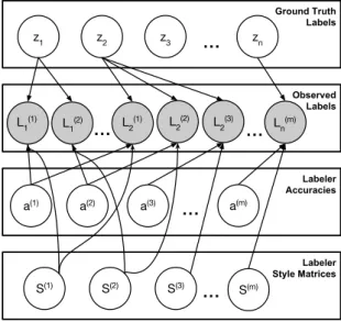
The dependence of the variables introduced in this section is shown graphically in Figure 4.1.

Ground Truth Labels Observed Labels Labeler Accuracies Labeler Style Matrices

...

...

...

...

...

Figure 4.1:Graphical model of ground-truth, observed labels, styles, and accuracies. Only the observed labels (shaded) are observed. The accuraciesa(1), . . . ,a(m)can be “folded” into the style matrices due to Lemma 4.1.

4.3

Likelihood Model

We define the probability that annotator iassigns labell_∈Ωto example j, given the ground-truth labelz, style matrixS, and accuracyaas:

p(L(_ji)=l|zj=z,S(i)=S,a(i)=a) . = a×Szl+(1−a)× ∑ z′_̸=zSz′l n₋1 = ⎛ ⎜ ⎜ ⎜ ⎜ ⎜ ⎝ S ⎡ ⎢ ⎢ ⎢ ⎢ ⎢ ⎣ a 1_n−₋a₁ . . . 1−a n−1 a 1−a n−1 . . . .. . . .. 1−a n−1 a ⎤ ⎥ ⎥ ⎥ ⎥ ⎥ ⎦ ⎞ ⎟ ⎟ ⎟ ⎟ ⎟ ⎠ zl (4.1)

CHAPTER 4. MODEL DESCRIPTION

The intuition is that there are two situations in which an annotator iwould respond with some particular label l: either (i) they correctly perceived the example as belonging to class z but transcribed it intol(i.e.,a×Szl), or (ii) they incorrectly perceived some other classz′but still

transcribed it intol(i.e., (1₋a)_×∑

z′_̸=zS_z′_l). Notice that, in either case, it is possible thatl=z.

We assume that the probability of an incorrect perceptionz′_̸=zis distributed uniformly over all (n₋1) incorrect classes.

4.4

Simplifying the Likelihood Model

Notice that, in Equation 4.1, the style matrix Sis right-multiplied by an accuracy matrix containingaon the diagonal and 1_n−a

−1 everywhere else. The accuracy matrix can easily be verified

to be a DSM. Moreover, by making use of a simple lemma, we can simplify our model: Lemma 4.1. Let A and B be two arbitrary DSMs. Then AB is also a DSM.

Proof. See Appendix A. ■

We can therefore “fold” the accuracy matrix into the style matrix, so that the latter expresses both the permutation and accuracy of the annotator. This enables us to simplify the likelihood model to be:

(4.2) p(L(_ji)=l|zj=z,S(i)=S)=Szl

This simplified model has an intuitive form. As opposed to a permutation matrix, which can only model discrete permutations, our model, utilizing a single DSM, can model a “soft” style whereby an annotator “usually” transcribes zintolbut may sometimes transcribe it intol′, etc.

4.5

Comparison to RSM-based Model

PICA is based on doubly-stochastic matrices (DSMs), which are a special case of right-stochastic matrices (RSMs) – non-negative matrices in which the rows, but not necessarily the columns, sum to 1. RSMs are therefore also capable of modeling the same kinds of “styles” that our proposed DSM-based model can model. RSM-based models for crowdsourcing consensus algorithms were first developed by [1]. Compared to RSM-based models, DSMs directly encode the fact that each annotator may permute his/her perception of the class into a different label. DSMs can have an advantage over RSMs due to a smaller number of degrees of freedom: where ann_×nRSM hasn(n₋1) free parameters, DSMs have only (n₋1)2, which for smalln(i.e., a small number of classes or clusters) can be substantial in relative terms. When collecting only a modest number of labels per annotator, this reduction in free parameters can lead to better estimation of each annotator’s style matrix and more accurate inference of the ground-truth labels.

4.6. COMPARISON TO UNPERMUTATION HEURISTIC

4.6

Comparison to Unpermutation Heuristic

A simple way to perform permutation-invariant consensus is to “un-permute” the labels based on similarities between annotators. For example, if for some subset of examples Annotator 1 uses label A and Annotator 2 uses label B, it is likely A and B refer to the same class. Based on this idea, we constructed the following algorithm – which we refer to as theUnpermutation Heuristic – and for which we provide comparative results in the following sections.

Algorithm:

• Randomly pick an annotator ias the “leader”. • Using i’s labels,

• For each annotator j_̸=i, • For each classk=1, ...,n

• Find the symbol used most frequently by j to express classk according to i’s labels

• Un-permute j’s labels based on the inferred permutation • Conduct majority vote over the unpermuted labels of all annotators

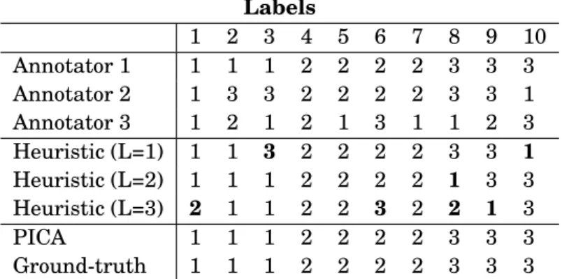
Recall the toy example presented in Figure 1.1 with the new set of observed labels given in Table 4.1. Annotator 1 is the same as in the previous example (perfect accuracy, identity style). Annotator 2 and 3 also have an identity style, but have low accuracy. PICA is able to identify this and again recovers the ground-truth labels with perfect accuracy. Conversely, the Unpermutation Heuristic misinterprets the low accuracy of Annotators 2 and 3 as a style transformation and makes several mistakes.

It is important to note that the performance of the Unpermutation Heuristic is highly sensitive to the choice of the “leader”. This isn’t surprising; unpermuting the other annotators’ labels based on the labels of an inaccurate leader will propagate the error. The results of the Unpermutation Heuristic for each possible choice of leader are given in Table 4.1. The accuracy of the Unpermutation Heuristic for each leader is 80%, 90%, and 60% respectively, while PICA scores 100%.

CHAPTER 4. MODEL DESCRIPTION Labels 1 2 3 4 5 6 7 8 9 10 Annotator 1 1 1 1 2 2 2 2 3 3 3 Annotator 2 1 3 3 2 2 2 2 3 3 1 Annotator 3 1 2 1 2 1 3 1 1 2 3 Heuristic (L=1) 1 1 3 2 2 2 2 3 3 1 Heuristic (L=2) 1 1 1 2 2 2 2 1 3 3 Heuristic (L=3) 2 1 1 2 2 3 2 2 1 3 PICA 1 1 1 2 2 2 2 3 3 3 Ground-truth 1 1 1 2 2 2 2 3 3 3

Table 4.1:With labels from inaccurate annotators, PICA perfectly recovers the ground-truth labels while the Unpermutation Heuristic makes mistakes regardless of the choice of leader.

C

H A P T E R

5

I

NFERENCE

Given the observed labelsL and our simplified likelihood model (Equation 4.2), we can use Expectation-Maximization to optimize over the style matrices of all the annotators and infer the ground-truth of each example. However, the constraint that each style matrix be doubly-stochastic requires special handling, which we describe in the M-Step section below.

The high-level intuition of our procedure is the following: in the E-Step, we compute our predictions (i.e. probabilities) for the label of each data example based on our current estimation of the annotators’ style matrices. Then in the M-Step, we modify our estimates of the style matrices to make them a more accurate reflection of the observed labels and our current predictions of the ground-truth labels. These steps are performed iteratively until accurate predictions of the style matrices and ground-truth labels have been reached.

Our derivations below make use of the conditional independence encoded in the graphical model in Figure 4.1.

5.1

E-Step

In this step, we compute the posterior probability distributions ofzj∈Ω∀j∈{1, . . . ,n}given

S(1), . . . ,S(m)from the last M-Step and the observed labelsL.

p(zj=zj|L(1)=L(1), . . . ,L(m)=L(m),

S(1)=S(1), . . . ,S(m)=S(m)) = p(zj|L(1), . . . ,L(m),S(1), . . . ,S(m))

CHAPTER 5. INFERENCE ∝ p(zj)p(L(1), . . . ,L(m)|S(1), . . . ,S(m),zj) = p(zj) ∏ i:L(_ji)̸=ϵ p(L(_ji)_|zj,S(i)) = p(zj) ∏ i:L(_ji)̸=ϵ S(i) zj,L(_ji)

where we note that p(z_j|S(1), . . . ,S(m))₌p(z_j) by conditional independence assumptions from the graphical model. Also, note thatS(i)

zj,L(_ji)

is thezjth row andL(_ji)th column ofS(i).

5.2

M-Step

In this step, we maximize the auxiliary functionQ, defined as the expectation of the joint log-likelihood of the observed labels and ground-truth labels, with respect to the posterior distribution of eachzjcomputed in the last E-Step, denotedp˜.

Q(S(1), . . . ,S(m)) = E[ logp(L₌L,z=z_|S=S) ] = E[ logp(L,z_|S) ] = E [ log∏ j ( p(zj) ∏ i p(L(_ji)_|zj,S(i)) )]

sinceL(_ji)are cond. indep.

= ∑ j E[ logp(z_j)]₊∑ i j E[ log(L(_ji)_|z_j,S(i))] = ∑ i j E[log(L(_ji)_|zj,S(i) )] +C since∑ j

E[logp(zj)] is const. w.r.t. eachS(i)

= ∑ i j ∑ z1 . . .∑ zd log(p(L(_ji)_|z_j,S(i)))p_˜(z₁, . . . ,z_d) = ∑ i j ∑ zj log(p(L(_ji)|zj,S(i)) ) ˜ p(zj) ∑ z1 · · ·∑ zj−1 ∑ zj+1 · · ·∑ zd ˜ p(z1, . . . ,zj−1,zj+1, . . . ,zd) = ∑ i j ∑ zj log(p(L(_ji)_|zj,S(i)) ) ˜ p(zj) = ∑ i j ∑ zj log ( S(i) z,L(_ji) ) ˜ p(zj)

Remark 5.1. Notice we drop the constant C after introducing it. Since this constant is the same for all values of S, it doesn’t need to be computed.

5.3. PRIOR ON STYLE

To take the first derivative ofQ, we vectorize eachS(i):

∂Q ∂vec[S(i)_]= [ _∂Q ∂S(₁₁i) . . . ∂Q ∂S(₁i_n) ∂Q ∂S(₂₁i) . . . ∂Q ∂S(nni) ] where ∂Q ∂S(_{x y}i) = ∑ j:L(_ji)̸=ϵ ∑ zj ∂ ∂S(_{x y}i)[log ( S(i) zj,L(ji) ) ]p_˜(zj) = ∑ j:L(_ji)̸=ϵ ∂ ∂S(_{x y}i)[log ( S(i) x,L(_ji) ) ]p_˜(x) = ∑ j:L(_ji)̸=ϵ δ(L(_ji),y) ∂ ∂S(_{x y}i)[log ( S(_{x y}i))]p_˜(x) = ∑ j:L(_ji)̸=ϵ δ(L(_ji),y)p˜(x) S(_{x y}i)

If S were a real-valued matrix, we could simply use a gradient ascent method (stochastic, conjugate, etc.) to find values ofS(1), . . . ,S(m)that maximizeQ. However, the constraint that each style matrix is doubly-stochastic requires a more specialized optimization method to ensure that the result of each gradient update remains on the Birkhoff polytope (i.e. the manifold whose points are DSMs). As discussed in Chapter 3, we can utilize Sinkhorn Propagation to satisfy the DSM constraints.

After conducting Expectation-Maximization, we take the final probability distribution, from the last E-Step, of eachzjas the estimated label for each example j.

5.3

Prior on Style

In some settings, we may also wish to add a regularization term to “push” the style matrices towards the identity permutation; this can be useful if most labelers are assumed to use some “default” permutation (identity). To do so, we can subtract fromQan additional term _nγ2∥S(i)−I∥2_Fr

where γ specifies the strength of the regularization, I is the identity matrix with the same dimensions as S(i) (i.e. n_×n), and _{∥ · ∥}2_Fr is the squared Frobenius norm. Similarly, for the derivative ∂Q

∂S(x yi)

C

H A P T E R

6

E

XPERIMENTS

6.1

Overview

We developed several experiments to evaluate our model. Our experiments fall under two categories: the first are simulations which were designed to highlight specific benefits of our model over other models. The second demonstrate the efficacy of our model in useful applications i.e. text passage clustering and dense image segmentation. In all of the experiments, we compute percent correct and cross-entropy as our performance metrics.

6.1.1 Permutation-invariant accuracy measurement

Since the cluster labels in our experiments have no inherent meaning (e.g., we could swap the labels “1” and “2” without changing any semantics of the clusters), we computed accuracy of the estimated cluster labels as themaximumaccuracy, over alln! permutations, of the estimates with respect to ground-truth cluster labels. As we focus on applications wherenis small, computing over alln! permutations is computationally feasible.

6.1.2 Optimization details

For all but the image segmentation experiment, we conducted Expectation-Maximization until Q(k)−Q(k−1)<10−4, whereQ(k)is the value ofQat thekth iteration. For the image segmentation experiment, we used a tolerance of 10−5_{. The code for the PICA model implementation as well as}

the experimental analyses is available athttps://github.com/mjgiancola/MQP.

6.2. TEXT PASSAGE CLUSTERING

6.2

Text Passage Clustering

6.2.1 Description

We designed a text passage clustering task which required annotators to cluster 6 passages into three groups (see Figure 6.1). This experiment was conducted on real annotators from Amazon Mechanical Turk. The workers were not told how many passages to put into each group, or by what characteristics to cluster them. They were told simply to “Determine how to group the passages based on any similarities and differences that you can identify”. Of the six text passages, two were in English, two were in Italian, and two were in Russian. We expected that most people would cluster by language, as the content of the passages were selected to be totally unrelated. (The passages were selected from Wikipedia articles on disparate topics such as mongoose, jet pack, Italian soccer players, etc.) See Figure 6.1 for the task description that we posed on Mechanical Turk.

Instructions

Below is a collection of passages of text in different lan-guages. The objective of this HIT is to collect the passages into three groups. Determine how to group the passages based on any similarities and differences that you can identify. To complete this HIT:

• Readallthe passages.

• Decide how to group the passages and go back to select a group for each passage.

Passages

1. Mongoose is the popular English name for 29 of the 34 species in the 14 genera of the family Her-pestidae, which are small feliform carnivorans native to southern Eurasia and mainland Africa.

⃝Group 1⃝Group 2⃝Group 3

2. Nicola Ventola (Grumo Appula, 24 maggio 1978), un ex calciatore italiano, di ruolo attaccante.

⃝Group 1⃝Group 2⃝Group 3 ...

6. L’oceano Indiano è un oceano della Terra. In par-ticolare, sia per superficie che per volume, tra i cinque oceani della Terra è il terzo.

⃝Group 1⃝Group 2⃝Group 3

Figure 6.1:The text passage clustering task we posted on Amazon Mechanical Turk. The annota-tors’ job was to group the different text passages into clusters.

CHAPTER 6. EXPERIMENTS

in 149 labels. Qualitatively, we observed that, while the majority of workers clustered by language, there was some noise in the data due to people clustering with some other reasoning in mind.

6.2.2 Results – Experiment 1

We assessed accuracy based on a randomly chosen subset (without replacement) of just 3 (out of 25) annotators, and then repeated the experiment 100 times to obtain an average performance estimate. Hence, the accuracy statistics we report reflect an annotation scenario in which only a small number of annotators provide labels, and the job of the aggregator is to infer the ground-truth labels despite the annotators’ differing styles.

The proposed PICA model (based on DSMs) achieved an average (over all 100 samplings) of 93% accuracy, with average cross-entropy (computed between the probability distributions of thezjwith respect to ground-truth labels) of 2.54. In contrast, the Unpermutation Heuristic

achieved an accuracy of only 90.5%, and simple Majority Vote scored 89%. This provides a simple proof-of-concept on labels from real human annotators that permutation-invariant consensus algorithms can be useful. The best performing model, however, was actually the RSM approach [1], which achieved an accuracy of 96% and cross-entropy of 1.65; this shows that the lower number of free parameters in DSMs may not always be decisive.

6.2.3 Results – Experiment 2

We again assessed accuracy based on a subset of the data, except this time we randomly sampled (without replacement) 2 labels from each of the 25 annotators, for a total of 50 observed labels in each experiment. In this set of experiments, there were many more observed labels but less per annotator, so being able to accurately infer the style of each annotator becomes more difficult and more important for accurately recovering the ground-truth labels.

Over 100 independent trials, PICA scored 94% with 6.31 cross-entropy, RSM scored 97% with 1.46 cross-entropy, the Unpermutation Heuristic scored 59%, and Majority Vote scored 91.67%. We find that RSM is slightly better than PICA yet again, although we see a significant performance difference from the Unpermutation Heuristic, which did not have enough data per annotator to make accurate inferences.

6.3

Rare Class Simulation

6.3.1 Description

This simulation was designed to highlight the difference between our DSM-based model and a simpler RSM-based model (e.g., [1]). Recall that, oncen−1 rows of ann×nDSM have been identified, then the last row can be inferred unambiguously. With RSMs, on the other hand, all of the rows must be inferred from data independently (since there is no constraint that each column

6.4. DENSE IMAGE SEGMENTATION

sums to 1). This difference can be decisive in a setting in which one of the classes (from {1, . . . ,n}) occurs only rarely in the dataset, so that few of the observed labels provide any information on the values of eachS(i).

For this simulation, we generated 100 examples, each of which was assigned a labelzj∈Ω={

‘a’, ‘b’, ‘c’ }, withp(‘a’)₌0.5, p(‘b’)₌0.45,p(‘c’)₌0.05. We then simulated 100 annotators who each have a random accuracya(i)sampled uniformly from [0.75, 1). Each annotator had a random permutation of the identity for their style matrix. For each annotator, we collected 10 labels, sampled randomly (without replacement) from the 100 total examples, giving a total of 1000 observed labels. As in the Text Passage Clustering experiments, results were averaged over 100 independent trials.

6.3.2 Results

The DSM-based PICA algorithm achieved a percent correct of 88% and 4.01 cross entropy, while the RSM-based model scored 79% with 6.32 cross entropy. As a baseline, the Unpermutation Heuristic scored 62% and Majority Vote scored 47%. These results show an example of how the more constrained DSM-based PICA algorithm can yield higher accuracy than the simpler (and less constrained) RSM-based approach.

6.4

Dense Image Segmentation

6.4.1 Description

In this experiment we explored whether PICA could reconstruct a dense (pixel-wise) image segmentation from multiple noisy segmentations. In our experiment, we used an image and ground-truth segmentation (Figure 6.2 (a-b)) from the ADE20K dataset [24], which in turn included images from the LabelMe dataset [25]. Based on the ground-truth segmentation, we then generated segmentations for 10 simulated annotators by permuting the class labels and adding noise (see Figure 6.2 (c) for an example). The input to our model thus consisted of

10×numPixelslabels, where each of the 10 segmentations corresponded to the labels of a single

annotator, and each pixel corresponded to an individual example (ie. pixel jin imageiis label L(_ji)). We generated a segmentation dataset for four different images: “couple”, “flag”, “light’, and “people”; the “couple” image is shown in Figure 6.2 (a). Together, these data enable us to assess whether PICA can infer each annotator’s different “style” in assigning pixels to colors and combine them across annotators to yield aggregated segmentations that are more accurate.

6.4.2 Results

Accuracy in inferring the ground-truth clustering labels with respect to the ground-truth of the four approaches – PICA (based on DSMs), RSM, the Unpermutation Heuristic, and Majority

CHAPTER 6. EXPERIMENTS

(a) (b) (c)

Original Image Ground-truth Noisy labeler

(d) (e) (f) (g)

PICA (DSM) RSM Baseline MV

Figure 6.2:A dense (pixel-wise) image segmentation task on one of the images (“couple”) from the ADE20K dataset [24]. Sub-figures a-f show (in order) the original image, the ground-truth segmentation, the segmentation collected from one of the simulated noisy labelers, and then the inferred ground-truth (over all 10 noisy labelers) using the proposed DSM-based PICA algorithm, the RSM-based algorithm [1], the baseline algorithm, and simple Majority Vote.

Vote – are shown in Table 6.1. Graphical results just for the “couple” image are also shown in Figure 6.2 (d)-(g). As with the previous experiments, we compute the %-correct accuracy and cross-entropy as themaximumover alln! permutations, wherenis the number of class labels. Hence, the accuracies of the models are not penalized due to just the arbitrary coloring assigned to each cluster in the image.

For the “couple” image, PICA was able to reconstruct the original segmentation with 100% accuracy. In contrast, the RSM model achieved 80% accuracy relative to the original segmentation, as it was unable to distinguish the foreground and background of the image. A simple majority vote still achieved 77% accuracy, but generates a segmentation with a lot of noise. For this example, the Unpermutation Heuristic achieved the same level of performance as PICA – this was expected as the simulated annotators were highly accurate.

The results for all four images we tested on are shown in Table 6.1. For three of the four images, PICA performed the best in terms of %-correct clustering accuracy (fraction of pixels assigned to the correct cluster, after taking the maximum over alln! permutations), tying with

6.4. DENSE IMAGE SEGMENTATION

Model Image

“couple” “flag” “light” “people”

% C.E. % C.E. % C.E. % C.E.

PICA 100 65.5 99.4 .077 99.8 .020 99.0 48.2

RSM 80.4 13.9 98.7 .139 99.1 .040 99.0 39.6

Heuristic 100 – 99.2 – 99.8 – 98.9 –

MV 77.5 – 81.5 – 88.9 – 86.0 –

Table 6.1:Accuracy of the proposed DSM-based PICA model compared to the RSM-based model [1] for aggregating over multiple annotators’ dense (pixel-wise) image segmentations. We applied both algorithms to four different images (“couple”, “flag”, “light”, and “people”). Accuracy was measured using %-correct accuracy in assigning pixels to clusters, as well as cross-entropy.

the Unpermutation Heuristic twice and with RSM once. In terms of cross-entropy, the results were more mixed, and both RSM and PICA achieved the best cross-entropy in two of the four images.

While this is simply a proof-of-concept, it illustrates how crowdsourcing – and principled algorithms for aggregating over crowdsourced labels – can be used for image segmentation tasks. After investigating annotation consistency between segmentations, [24] discussed the important sources of error. The first was varying levels of segmentation quality from different annotators. The second was ambiguities in object naming (ie. one annotator labeled a truck as “car”). As shown empirically, the proposed PICA model can construct a segmentation which eliminates the noise in the given data. The object naming issue would be eliminated entirely, as PICA is invariant to each annotator’s style.

C

H A P T E R

7

C

ONCLUSION

This paper presented a crowdsourcing consensus algorithm called PICA (Permutation-Invariant Crowdsourcing Aggregation) which performs permutation-invariant simultaneous inference of the ground-truth labels and the individual annotators’ styleof labeling. This al-lows our model to excel in scenarios when annotators havesystematic confusionsof what the different classes mean, or when the particular class labels don’t matter (e.g. clustering, image segmentation).

We modeled style using a doubly-stochastic matrix (DSM) for each annotator, whose entries gave the probability that the annotator perceived some latent class, but transcribed another. We then utilized Sinkhorn Normalization [5] and Sinkhorn Propagation [4] to find the optimal style matrix for each annotator, within an Expectation-Maximization-based optimization scheme.

In contrast to [1], our model can benefit from harnessing a smaller number of degrees of freedom to reduce overfitting. Namely, PICA outperformed the RSM-based model [1] in a simulated experiment where there were a relatively small number of examples from one class.

We evaluated our model on simulated image segmentation data [24] and found that PICA was able to perfectly reconstruct an image segmentation based on several noisy segmentations.

7.1

Future Work

An interesting area of future inquiry is exploring the relationship between the number of annotators and examples in some labeling task. One would expect that the number of annotators and examples have an inverse relationship in the sense that having more annotators can compen-sate for having fewer labels per annotator. But is there a limit to the extent that more examples can make up for a lack of annotators (and vice-versa)? For the particular case of PICA, it would be

7.1. FUTURE WORK

interesting to investigate how this issue interacts with the relative benefits/drawbacks of using DSM-based versus RSM-based models.

As our work on image segmentation was simulated, it would be interesting to see how PICA performs on real data i.e. aggregating the labels from several annotators to create a consensus segmentation. One challenge will be to quantify the results. In our work, we were able to compare the models’ performances to the “ground-truth” i.e. the original segmentation from which the noisy segmentations were generated. However on real data, there would be no ground-truth to compare to, so the results of such experiments would likely be more qualitative.

Appendices

A

P P E N D I X

A

DSM

S

C

LOSED

U

NDER

D

OT

P

RODUCT

Lemma 4.1:Let A and B be two arbitrary DSMs. Then AB is also a DSM. Proof. Let AandBbe two arbitrary DSMs.

A₌ ⎡ ⎢ ⎢ ⎢ ⎢ ⎢ ⎣ a11 a12 . . . a1n a21 a22 . . . a2n .. . an1 an2 . . . ann ⎤ ⎥ ⎥ ⎥ ⎥ ⎥ ⎦ B₌ ⎡ ⎢ ⎢ ⎢ ⎢ ⎢ ⎣ b11 b12 . . . b1n b21 b22 . . . b2n .. . bn1 bn2 . . . bnn ⎤ ⎥ ⎥ ⎥ ⎥ ⎥ ⎦

Column jofABhas the form:

AB_∗j= ⎡ ⎢ ⎢ ⎢ ⎢ ⎢ ⎣ a11b1j+a12b2j+ · · · +a1nbn j a21b1j+a22b2j+ · · · +a2nbn j .. . an1b1j+an2b2j+ · · · +annbn j ⎤ ⎥ ⎥ ⎥ ⎥ ⎥ ⎦

Taking the sum of the elements in column j, we can reorder the terms and find:

b1j(a11+ · · · +an1) +b2j(a12+ · · · +an2) +. . . +bn j(a1n+ · · · +ann) =b₁j+b2j+ · · · +bn j =1

A

P P E N D I X

B

E

XAMPLE OF

O

NE

S

INK

P

ROP

I

TERATION

This appendix contains a simple, illustrative example of how Sinkhorn Propagation is per-formed. We start with a strictly positive matrix A1, perform one Sinkhorn iteration (ie. one row normalization and one column normalization), and compute the value of a function f (sum of squares) of our (almost) DSM. Then we compute the gradient _∂∂_Af using Sinkhorn Propagation.

LetA= [ 2 5 3 4 ] and f =∑2 i=1 ∑2 j=1A 2 i j. ThenR(A)₌ ⎡ ⎣ 2 7 5 7 3 7 4 7 ⎤ ⎦,C(R(A))= ⎡ ⎣ 2 5 5 9 3 5 4 9 ⎤ ⎦, and f(C(R(A)))=1₂₀₂₅53 ≈1.026

Next, we compute _∂∂_Af by “back-propagating” the gradient through the Sinkhorn iterations. Notice we have vectorized the matrices so that _∂vec[∂f_C] has shape 1×n2, _∂vec[∂C_R] has shapen2×n2, and _∂vec[∂R_A] has shapen2_×n2.

∂f ∂vec[C]=2∗vec[C]= [ 4 5 10 9 6 5 8 9 ] ∂C ∂vec[R]= ⎡ ⎢ ⎢ ⎢ ⎢ ⎢ ⎢ ⎢ ⎣ ∂C11 ∂R11 ∂C12 ∂R11 ∂C21 ∂R11 ∂C22 ∂R11 ∂C11 ∂R12 ∂C12 ∂R12 ∂C21 ∂R12 ∂C22 ∂R12 ∂C11 ∂R21 ∂C12 ∂R21 ∂C21 ∂R21 ∂C22 ∂R21 ∂C11 ∂R22 ∂C12 ∂R22 ∂C21 ∂R22 ∂C22 ∂R22 ⎤ ⎥ ⎥ ⎥ ⎥ ⎥ ⎥ ⎥ ⎦ = ⎡ ⎢ ⎢ ⎢ ⎢ ⎢ ⎢ ⎢ ⎣ 21 25 0 − 14 25 0 0 28₈₁ 0 −₈₁35 −21 25 0 14 25 0 0 −₈₁28 0 35₈₁ ⎤ ⎥ ⎥ ⎥ ⎥ ⎥ ⎥ ⎥ ⎦

1_{To make the computations simpler, we exclude the exp(A) step in this example.}

∂R ∂vec[A]= ⎡ ⎢ ⎢ ⎢ ⎢ ⎢ ⎢ ⎢ ⎣ ∂R11 ∂A11 ∂R12 ∂A11 ∂R21 ∂A11 ∂R22 ∂A11 ∂R11 ∂A12 ∂R12 ∂A12 ∂R21 ∂A12 ∂R22 ∂A12 ∂R11 ∂A21 ∂R12 ∂A21 ∂R21 ∂A21 ∂R22 ∂A21 ∂R11 ∂A22 ∂R12 ∂A22 ∂R21 ∂A22 ∂R22 ∂A22 ⎤ ⎥ ⎥ ⎥ ⎥ ⎥ ⎥ ⎥ ⎦ = ⎡ ⎢ ⎢ ⎢ ⎢ ⎢ ⎢ ⎢ ⎣ 5 49 − 2 49 0 0 −5 49 2 49 0 0 0 0 ₄₉4 −₄₉3 0 0 −₄₉4 ₄₉3 ⎤ ⎥ ⎥ ⎥ ⎥ ⎥ ⎥ ⎥ ⎦ Using Equation (3.1), ∂f ∂A≈ [ −0.042 0.017 0.026 ₋0.020 ]

Notice if we apply this gradient to A, we get A′_≈

[

1.958 5.017 3.026 3.98

]

and f(C(R(A′)))_≈1.028, which is a slight improvement from our original A.2

2_{Notice, the optimal DSM matrix forf is the identity (or some transformation of it), which will produce the value}

A

P P E N D I X

C

D

ATA

C

OLLECTION

C.1

Text Passage Clustering Data

We collected passages on Wikipedia for our text clustering experiment. Since we wanted passages in multiple languages, we used English, Russian, and Italian Wikipedia articles. The passages we used came from the following articles: Mongoose and Jet Pack (English), Nicola Ventola and Indian Ocean (Italian), and Ludwig van Beethoven and G-Eazy (Russian).

C.2

Image Segmentation Data

We used an image and segmentation from the ADE20K dataset [24]. The image was originally from the LabelMe dataset [25]. To reduce time costs, we cropped sections of the image to use. Also, to simplify the results, we regenerated our own segmentations which ignored a few class labels (ie. small objects in the background).

B

IBLIOGRAPHY

[1] Padhraic Smyth, Usama M Fayyad, Michael C Burl, Pietro Perona, and Pierre Baldi. Inferring ground truth from subjective labelling of venus images.

InAdvances in neural information processing systems, pages 1085–1092, 1995. [2] Michael Giancola, Randy Paffenroth, and Jacob Whitehill.

Permutation-invariant consensus over crowdsourced labels.

InSixth AAAI Conference on Human Computation and Crowdsourcing, 2018. [3] Paul Ekman.

All emotions are basic.

The nature of emotion: Fundamental questions, pages 15–19, 1994. [4] Ryan Prescott Adams and Richard S Zemel.

Ranking via sinkhorn propagation. arXiv preprint arXiv:1106.1925, 2011. [5] Richard Sinkhorn.

A relationship between arbitrary positive matrices and doubly stochastic matrices. The annals of mathematical statistics, 35(2):876–879, 1964.

[6] Richard Sinkhorn and Paul Knopp.

Concerning nonnegative matrices and doubly stochastic matrices. Pacific Journal of Mathematics, 21(2):343–348, 1967.

[7] Alexander Philip Dawid and Allan M Skene.

Maximum likelihood estimation of observer error-rates using the em algorithm. Applied statistics, pages 20–28, 1979.

[8] Jacob Whitehill, Ting-fan Wu, Jacob Bergsma, Javier R Movellan, and Paul L Ruvolo. Whose vote should count more: Optimal integration of labels from labelers of unknown

expertise.

InAdvances in neural information processing systems, pages 2035–2043, 2009.

[9] Vikas C Raykar, Shipeng Yu, Linda H Zhao, Gerardo Hermosillo Valadez, Charles Florin, Luca Bogoni, and Linda Moy.

BIBLIOGRAPHY

Learning from crowds.

Journal of Machine Learning Research, 11(Apr):1297–1322, 2010. [10] Mahyar Salek, Yoram Bachrach, and Peter Key.

Hotspotting-a probabilistic graphical model for image object localization through crowd-sourcing.

InAAAI, 2013.

[11] Jonathan Bragg, Daniel S Weld, et al.

Crowdsourcing multi-label classification for taxonomy creation.

InFirst AAAI conference on human computation and crowdsourcing, 2013. [12] Yuyin Sun, Adish Singla, Dieter Fox, and Andreas Krause.

Building hierarchies of concepts via crowdsourcing. InIJCAI, pages 844–853, 2015.

[13] Christopher H Lin, Daniel Weld, et al.

Crowdsourcing control: Moving beyond multiple choice. arXiv preprint arXiv:1210.4870, 2012.

[14] Yuandong Tian and Jun Zhu.

Learning from crowds in the presence of schools of thought.

InProceedings of the 18th ACM SIGKDD international conference on Knowledge discovery and data mining, pages 226–234. ACM, 2012.

[15] Ece Kamar, Ashish Kapoor, and Eric Horvitz.

Identifying and accounting for task-dependent bias in crowdsourcing.

InThird AAAI Conference on Human Computation and Crowdsourcing, 2015. [16] Nam Nguyen and Rich Caruana.

Consensus clusterings.

InData Mining, 2007. ICDM 2007. Seventh IEEE International Conference on, pages 607– 612. IEEE, 2007.

[17] Alexander Topchy, Anil K Jain, and William Punch.

Clustering ensembles: Models of consensus and weak partitions.

IEEE transactions on pattern analysis and machine intelligence, 27(12):1866–1881, 2005. [18] Alexander Strehl and Joydeep Ghosh.

Cluster ensembles—a knowledge reuse framework for combining multiple partitions. Journal of machine learning research, 3(Dec):583–617, 2002.

[19] Amir Alush and Jacob Goldberger.

BIBLIOGRAPHY

Ensemble segmentation using efficient integer linear programming.

IEEE transactions on pattern analysis and machine intelligence, 34(10):1966–1977, 2012. [20] Oded Kaminsky and Jacob Goldberger.

Combining clusterings with different detail levels.

InMachine Learning for Signal Processing (MLSP), 2016 IEEE 26th International Workshop on, pages 1–6. IEEE, 2016.

[21] Ryan G Gomes, Peter Welinder, Andreas Krause, and Pietro Perona. Crowdclustering.

InAdvances in neural information processing systems, pages 558–566, 2011. [22] Jinfeng Yi, Rong Jin, Shaili Jain, Tianbao Yang, and Anil K Jain.

Semi-crowdsourced clustering: Generalizing crowd labeling by robust distance metric learn-ing.

InAdvances in neural information processing systems, pages 1772–1780, 2012. [23] Ramya Korlakai Vinayak and Babak Hassibi.

Crowdsourced clustering: Querying edges vs triangles.

InAdvances in Neural Information Processing Systems, pages 1316–1324, 2016.

[24] Bolei Zhou, Hang Zhao, Xavier Puig, Sanja Fidler, Adela Barriuso, and Antonio Torralba. Scene parsing through ade20k dataset.

InProceedings of the IEEE Conference on Computer Vision and Pattern Recognition, 2017. [25] Bryan C Russell, Antonio Torralba, Kevin P Murphy, and William T Freeman.

Labelme: a database and web-based tool for image annotation. International journal of computer vision, 77(1-3):157–173, 2008.