Locally decodable source coding

(1)

Locally Decodable Source Coding

by

Ali Makhdoumi

JUL 0 8 2013

L IBRA RIES

Submitted to the Department of Electrical Engineering and Computer

Science

in partial fulfillment of the requirements for the degree of

Master of Science in Computer Science and Electrical Engineering

at the

MASSACHUSETTS INSTITUTE OF TECHNOLOGY

June 2013

@

Massachusetts Institute of Technology 2013. All rights reserved.

A uthor . . . -.- . .-...

Department of Electrical Engineering and Computer Science

May 20, 2013

Certified by

Certified by ....

/

Prof. Muriel M6dard

EECS Professor

Thesis Supervisor

. . . .

Prof. Yury Polyanskiy

EECS Assistant Professor

Thesis Supervisor

Accepted by...

_... _. _. _{. .} _{. .} _7...

Profkssor Lse A. Kolodziejski

Chair, Department Committee on Graduate Students

(2)

(3)

I/-Locally Decodable Source Coding

by

Ali Makhdoumi

Submitted to the Department of Electrical Engineering and Computer Science on May 20, 2013, in partial fulfillment of the

requirements for the degree of

Master of Science in Computer Science and Electrical Engineering

Abstract

Source coding is accomplished via the mapping of consecutive source symbols (blocks) into code blocks of fixed or variable length. The fundamental limits in source coding intro-duces a tradeoff between the rate of compression and the fidelity of the recovery. However, in practical communication systems many issues such as computational complexity, mem-ory capacity, and memmem-ory access requirements must be considered. In conventional source coding, in order to retrieve one coordinate of the source sequence, accessing all the encoded coordinates are required. In other words, querying all of the memory cells is necessary. We study a class of codes for which the decoder is local. We introduce locally decodable source coding (LDSC), in which the decoder need not to read the entire encoded coordi-nates and only a few queries suffice to retrieve a given source coordinate. Both cases of having a constant number of queries and also a scaling number of queries with the source block length are studied. Also, both lossless and lossy source coding are considered. We show that with constant number of queries, the rate of (almost) lossless source coding is one, meaning that no compression is possible. We also show that with logarithmic number of queries in block length, one can achieve Shannon entropy rate. Moreover, we provide achievability bound on the rate of lossy source coding with both constant and scaling num-ber of queries.

Thesis Supervisor: Prof. Muriel M6dard Title: EECS Professor

Thesis Supervisor: Prof. Yury Polyanskiy Title: EECS Assistant Professor

(4)

(5)

Acknowledgments

I would like to thank my advisors Prof. Muriel Medard and Prof. Yury Polyanskiy. I value

our discussions on different research challenges as well as their insightful guidance. They have been extremely supportive mentors, both professionally and personally. I also want to thank Mr. Shao-Lun Huang for his valuable comments on this thesis. I am also grateful to Prof. Pablo Parrilo, my academic mentor, for his valuable advices during my master study. I could not have come this far without the love of my family. I am always grateful to my parents, my sisters, and my wonderful friends for theirs endless love and support.

(6)

(7)

List of Figures

1-1 Typical structure of a communication system . . . 12

2-1 Locally Encodable Source Coding . . . 19

2-2 Locally encodable Source Coding: Definition of Locality . . . 20

3-1 Locally Decodable Source Coding . . . 26

3-2 Comparison of approximations of upper bounds, p = .11, d = 1/15 . . . . 43

3-3 Comparison of approximations of upper bounds, p = .11, d = 1/20 . . . . 44

(10)

(11)

Chapter 1 Introduction

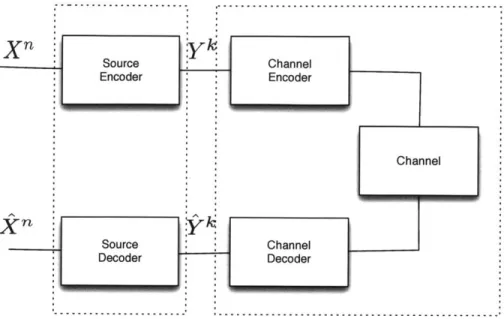
The block structure of a typical communication system is illustrated in 1-1. The source gen-erates a sequence Xn, the source encoder maps the sequence, X", into the bitstream, yk.

The bitstream is transmitted over a possibly erroneous channel and the received bitstream

frk

_{is processed by the source decoder in order to produce the decoded source sequence}

k n

The error probability of the channel is controlled by the channel encoder, which adds redundancy to the bits at the source encoder output, yk. Typically, there is a modulator and a demodulator. The modulator maps the channel encoder output to an analog signal, which is suitable for transmission over a physical channel. The demodulator interprets the received, often analog, signal as a digital signal, which is fed into the channel decoder. The channel decoder processes the digital signal and produces the received bitstream yk, which

may be identical to yk even in the presence of channel noise. According to separation

results [23, 22], source coding and channel coding can be constructed separately without loss of throughput in the overall system. The focus of this work is on the source encoder

and decoder parts. This part of communication system is called source coding. The main

goal of source coding is to compress data source in a way to be recoverable with a high

(12)

X"'Y

Source Channel Encoder Encoder Channel Source Channel Decoder Decoder

Figure 1-1: Typical structure of a communication system

1.1 Motivation

The basic communication problem may be expressed as transmitting source data with a high fidelity without exceeding an available bit rate, or it may be expressed as transmitting the source data using the lowest bit rate possible while maintaining a specified reproduction fidelity [23]. In either case, a fundamental trade-off is made between bit rate and distor-tion/error level. Source coding is primarily characterized by rate and distortion /error of the code. However, in practical communication systems, many issues such as computational

complexity, memory limitation, memory access requirements must be considered. For

in-stance, in a typical system, a small change in one coordinate of the input sequence leads to a large change in the encoded output. Moreover, in order to retrieve one symbol of the source sequence, accessing all the encoded coordinates are required. The latter issue is the main topic of this work.

One way to confront these issues is to place constraints on the encoder/decoder. In particular, in order to address the issue of memory access requirement, we study a class of codes for which the decoder is local (in a sense that will be defined later). A long line of research has addressed a similar problem from a data structure perspective. For example, Bloom filters [2] are a popular data structure for storing a set in a compressed form while

(13)

allowing membership queries to be answered in constant time. The rank/select problem

[18, 8] and dictionary problem in the field of succinct data structures are also examples of

problems involving both compression and the ability to efficiently recover a single element of the input. In particular, [20] gives a succinct data structure for arithmetic coding that supports efficient recovery of source. Reference [3] studies both issues at the same time and introduces a data structure with is efficient in both updating and querying. In all of these works the efficiency is interpreted in terms of the decoding time whereas in this work it is interpreted in terms of memory access requirement. In this work, we formulate this problem from an information theoretic view and study the fundamental trade-offs between locality and the rate of source coding.

A topic closely related to source coding with local decoding is the problem of source coding

with local encoding. This problem has been studied in many works in both data structure and information theoretic literatures. This line of research addresses the following chal-lenge: In order to be able to update an individual source symbol efficiently, we must study compression schemes that have some continuity property, meaning that a change in a single coordinate of the input sequence leads to a small change in the encoded sequence. Varsh-ney et al. [25] analyzed continuous source codes from an information theoretic point of view. Also, Mossel and Montanari [16] have constructed source codes based on nonlinear sparse graph codes. Sparse linear codes has been studied by Mackay [13], in which a class of local linear encoders are introduced. Also, Mazumdar et. all. [15] has studied update efficient codes which studies channel coding problem with local encoders.

Causal Source Coding is another close topic to source coding with local decoder, which

studies the source coding problem with causal encoder/decoder. In causal source coding the constraint on the decoder is not being local, but, being causal [17, 9].

Locally decodable codes (LDC) ([26]) is another close topic to source coding with local

decoder. An LDC encodes n-bit source sequence to k-bit codewords in such a way that one can recover any bit xi from a corrupted codeword by querying only a few bits of that codeword. Therefore, LDC introduces redundancy to combat the corruption of the code word.

(14)

yis, face erasure with some erasure probability. The goal is to produce another y, to re-place a erased yj, by accessing a few number of ys. Reference [19] introduces a trade-off between locality, code distance, and the rate of code.

(15)

Chapter 2 Background and Literature Review

In this chapter we present some fundamental concepts of source coding. We introduce the class of Locally Encodable Source Coding (LESC) which studies the problem of source coding with a local encoder. Also, we overview the results of Succinct Date Structure. In the next chapter we shall revisit these results from an information theoretic point of view and compare them to our results.

2.1 Source Coding

The primary task of source coding is to represent a source with the minimum number of (binary) symbols without exceeding an acceptable level of distortion, which is determined

by the application. Two types of source coding techniques are typically named almost

lossless source coding and lossy source coding.

2.1.1 Almost Lossless Source Coding

Almost Lossless Source Coding refers to a type of source coding that allows the exact reconstruction of the original source from the compressed data for almost all the source outputs. Almost lossless source coding are also called asymptotically lossless source cod-ing or some times by the abuse of name we call them lossless codcod-ing. Although that lossless compression such as Lempel-Ziv [28] exists and is generally markedly different in

(16)

construction. Lossless source coding can provide a reduction in bit rate compared to the original source, when the original data source contains dependencies or statistical proper-ties such as redundancy, sparsity, and correlation that can be exploited for data compression

. A well-known use for this type of compression for picture and video sources is JPEG-LS.

Next, a fundamental bound for the minimum average codeword length per source symbol that can be achieved with lossless coding is introduced. Let X C X be a random variable with probability measure IPx, where X is a finite alphabet set. Also let X" denotes n i.i.d copies of X.

Definition 1. An (n, k, e)-SC is a pair consist of encoder

f

: X" {0, 1}k and decoder g : {0, 1}k k X" such that jP[gyf (X")) -f X"] <e Also let k*c(n, c) Aminf k :3 (n, k, c) - SC}, kcksc(n, E) Rsc (n, c) = and Rsc (c) lim sup Rsc(n, c). n-*oo The rate is Rsc lim Rsc (c),

where SC stands for source coding.

For any X with probability measure Px, we have

Rsc = H(X), (2.1)

where H(X) denotes the entropy of a random variable ([4], chapter 5). The following theorem from [11, 24] characterizes the finite block length results on the rate.

(17)

Theorem 1. ([11, 24]) For any X with probability measure Px, we have

Rsc(n, c) = H(X) + =(X)Ql(c) + E( log), (2.2)

n n

where V(V) Var(log Px(X)) and

Q-

1 is the functional inverse of the Q-function, where Q(x) = e2dy.

-2.1.2

Lossy Source Coding

Lossy source coding refers to a type of source coding where a source is represented by a loss of information. In this case, only an approximation of the original source can be reconstructed from the compressed data. Lossy coding is the primary coding type for the compression of speech, audio, picture, and video signals, where an exact reconstruction of the source data is not required. A well-known application of lossy coding techniques is

JPEG. A measure of the quality of the approximation, is referred to as the distortion.

The minimum number of bits per source symbol that are required for representing a given source without exceeding a given distortion level is called rate distortion.

To measure the quality of an approximation, distortion measures are defined to express the differences between a reconstructed source and the corresponding original data source as a non-negative real value. A smaller distortion corresponds to a higher approximation quality. A distortion of zero specifies that the reproduced symbols are identical to the cor-responding original symbols. In this work, we restrict our considerations to the important class of additive distortion measures. The distortion between a single reconstructed symbol

e

E

Zand

_{the corresponding original symbol x E X is dened as a function d(x, ^) > 0,} with equality if and only if x = ,. Given such a distortion measure d(x, ), the distortion

between a sequence JP and x" is defined as

d(X",4_) = d(i, i).

i=1

For binary sources where X = X = {0, 1}, the most commonly used additive distortion

(18)

of an average distortion code for a given source.

Definition 2. A (n, k, D)-LSC is a pair consist of an encoder

f

: X" - {0, 1}" and a

decoder g : {0, 1}k _+ X" such that

E [d(X" n I " )] < D. Let

k* (, D) A min{k : (n, k, D) -LSC},

Risc(n, D) A k*,(n, D)

n

and the rate is

R18c(D) A lim sup Risc(n, D),

n-+oo

where lsc stands for lossy source coding.

For any X with probability measure Px, the characterization of the rate distortion is given by ([4], chapter 10)

Rsc (D) = min

E[d(X,X)]<D

I(X;

Z).

(2.3)

The following theorem characterizes the finite block length results on the rate of lossy source coding.

Theorem 2. ([27]) For any X with probability measure Px, we have

log n

n (2.4)

Risc(n, d) Risc(D) + _nn

where Rise(D) is given in (2.3).

We shall use the finite length results in the next chapters when we study locally decod-able lossy source coding.

(19)

deg <t deg<t

source:

xX2

X

encoded:

_Y

_Y2 _~~~~~~~~~ _Y

decoded:

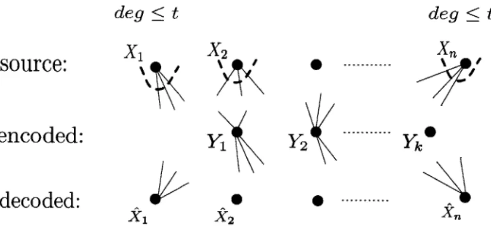
0 0

---Figure 2-1: Locally Encodable Source Coding

2.2 Locally Encodable Source Coding

We term Locally Encodable Source Coding (LESC) source coding where the encoder is local (The name that we use is not found the literature). In particular, [13, 16] study the case where, for any i, Xi influences only a constant number (t) of Ys. This class of source codes is depicted in Figure 2-1. In this figure, we connect Y to X, if Xj contributes to evaluate Y (we shall define this formally later). As shown in the figure, the source nodes have bounded degree determined by the locality. In this section, we formally define LESC and give the results in the literature for both lossless and lossy settings.

2.2.1 Lossless LESC

A lossless coding is defined as a pair of encoder

f

and decoder g, where,

f

: X -+ {0, I}k

and g : {0, 1}k _{X". The encoder is called local if each coordinate of the input affects a}

bounded number of coordinates of output. Formally, Let fa, for a E

{

1, ..., k}, be the a-th

component of the encoding function. Assume fa depends on Xn only through the vector

XAT= {Xy

j

E /} for some

N

c {1, ..., n}. Also for i E {1, ..., n}, let A be the set of output coordinates that depend on i. Thus,

(20)

source:

encoded:

decoded:

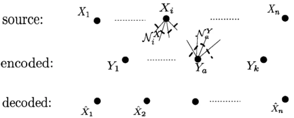
X1 xi 0 y₁ 0 0 Ya 0 0

Figure 2-2: Locally encodable Source Coding: Definition of Locality

For any given t, an encoder is called t-local if I| I t for any i E {1, ... , n}. Figure 2-2

illustrates

NV'

and X.

Definition 3. An (n, k, t, c)-LESC is a pair consisting a t-local encoder f : X"

-{0, I} and a decoder g : {0, I}k F X", such that Ip[g(f (X")) -f X" ] < E. Also, define

kg*(n, t, E) 4 min{k : (n, k, t, c) - LESC},

akg* (n, t, c)

Re (t, E)= lim sup ,

n-ioo n

and

Rie(t) 4 lim Rie (t, E),

C-40

where the subscript le stands for local encoder.

Next, we present relevant results in the literature about source coding with a local en-coder.

Assume a Bernoulli(p) i.i.d. source. The following result is derived in [13].

Theorem 3 (Mackay, very good codes, [13]). Assume X is a Bern(p) i.i.d. source with entropy h(p). For any given rate R > h(p), there exists an integer t(h(p), R) ;> 3 such that for any desired block error 6 > 0, there exists an integer no such that for any n > no there

exists a (n, nR, t (h(p), R) , 6) -LESC. Moreove, this encoder is a linear encoder.

Note 1. A Linear encoder for a Bernoulli source is a binary n x k matrix G such that Y = XG mod 2. This encoder is t-local if the weight of each row is at most t.

Xn 0

Yk*

xn ---..

(21)

Given a Bern(p) i.i.d. source and any rate R > h(p), we have Rie(t(h(p), R), E) < R.

Therefore, Rie(t(h(p), R)) < R. As a result, for any R > h(p), there exists t = t(h(p), R)

such that Rie (t) = R. Thus, we obtain a rate arbitrarily close to entropy using LESC. But,

in order to approach the entropy rate the locality must increase.

Source coding with local encoding is also studied in [16], considering a non-linear encoding function. In order to state the results we need the following definition. Let X be a source taking values from a finite set X. For any integer k > 1, let Dk(X) denote the set of probability measures Px over X, such that there exists a function

f

: Xk 1-+ X for

which the following holds. If X1, ... , Xk are i.i.d with measure Px, then f(X') is uniform

in X. Clearly, Dk(X) is finite and increasing in k, and D(X) = UkDk(X) is dense in the

X - 1 -dimensional simplex of probability measures over X.

The main result of [16] is as following.

Theorem 4 ([16]). Let X be a an i.i.d source over X with probability measure Px. If Px C D k(X), then there exists t*(Px) such that for any t > t*(Px) we have

H(Px) = inf { R : 3 LESC with rate R and t - local encoder}.

This theorem shows that, if the probability measure of the source comes from D(X)

(

a dense set on the space of probability distributions), then LESC achieves the fundamental limit, H(X).

Note 2. Unlike Theorem 3, the encoder proposed in Theorem 4 is not linear Moreover; in Theorem 3, in order to approach entropy, we need to increase the locality t. In other words, the locality, t, is a

function

of both rate and probability measure, whereas in Theorem 4 the locality is only a

function

of probability measure.

The number of queries, t can also be a growing function of the block length, n. We shall consider this case later.

(22)

2.2.2 Lossy LESC

Let

f

: X" + {0, 1}k and g :{, 1}' Il X be encoder and decoder, respectively. The encoder is called local if each coordinate of the input affects a bounded number of coordinates of output. This definition is the same as the previous one. Note that X E X and X E . Assume a probability measure on X, Px. A separable distortion measure

d : X x X i-+ R+ is given.

An (n, k, t, D)-LELSC is a pair consisting of a t-local encoder

f

: Xn - {O, 1}k

and a decoder g : {0, I}k _

Z",

such that E[d(X",

Z")]

< D. Also, define k*(n, t, D) - min{k : (n, k, t, D) - LESC},

and

a kg*(n, t, D)

Rie(t, D) = lim sup .

n-+oo n

Next, we state the relevant results in the literature about lossy source coding with local encoder.

Dimakis et. al. [7] discuss the case where the source has an i.i.d. Bern(!) distribution. The following theorem from [7] states that, if we choose the linear encoder generating matrix randomly, then with high probability the achievable rate by linear local encoder is bounded away from Shannon rate distortion. A Low Density Generating Matrices (LDGM) is used to guarantee locality. An LDGM is a Gnx matrix that maps sequences of length n to sequences of length k. It has locality (low density) of t if each row of it has at most t non-zeros.

Theorem 5 ([7]). Let X be a i.i.d source with Bern(!) distribution. Consider linear encoders that are chosen randomly from the set of all LDGMs with locality t . With high probability (wrt the ensemble) the achieved rate-distortion pair (R, D) satisfies:

Rie(t, D) > (1 - h(D)) 1 (2.5)

1 - exp

(verage

(2r5)

(23)

can achieve and does not apply to individual codes. The authors of [12] generalized this result by using a counting argument to individual linear local encoders. They showed that, for any linear local encoder with locality t, the performance is strictly bounded away from the Shannon rate-distortion function. However, the rate approaches rate-distortion as t increases. Formally,

For any R > 1-h(D), there exists t(R), such that the rate R can be achieved with locality t. Note that here, in order to approach the Shannon rate distortion function, we should in-crease the locality, t.

2.3 Succinct Date Structure

The problem of locally decodable (efficiently recoverable) compressed data structure (also called succinct data structure) is studied in many works from a database point of view. In succinct data structures we are concerned with the design of space efficient and dynamic data structures for storing a data source. We need the source data to be represented as compactly as possible to minimize storage, which is often highly constrained in these sce-narios. On the other hand, we wish to retrieve any coordinate of data source efficiently . Therefore, we are interested in data structures for storing sequences of length n produced

by a source in a compressed manner and being able to read the source coordinates

effi-ciently. Reference [20, 3] study this problem and the authors develop space bounds for data compression, i.e. storing a sequence of integers in a compressed binary format. They additionally seek to design compressed data indices to decode any small portion of the data or search for any pattern as a substring of the data, without decompressing the binary stored sequence entirely. Patrascu, [20] considered the problem of mapping a sequence, Xn, into a sequence, yk, and recovering X" from yk, where any sj only depends on O(log n) of Yis. This approach is very close to our locally decodable source coding scheme. We shall state the following result in the literature, in order to compare it to the results of LDSC in next chapter.

(24)

Theorem 6. ([20]) Consider a sequence of n elements from an alphabet X, and let

fx

be the number of occurrences of letter x in the sequence. On a RAM with cells of (log n) bits, we can represent the sequence by

O(|X log n) + E

fx

log( ) + n , + O(n3/4 log n3/4)

xeX ~

fX'

gI & ) +On3 4lo 3

bits of memory, supporting single-element access in 0(t). Each RAM is a sequence of bits with length O(log n). Single-element access in 0(t), means that each coordinate of the input sequence can be recovered by reading from 0(t) RAMs.

We shall elaborate on this result and reformulate it in a information theoretic form in the next chapter, where we shall develop the machinery to provide information theoretic explanation of succinct data structure, and in particular of Theorem 6.

(25)

Chapter 3 Locally Decodable Source Coding

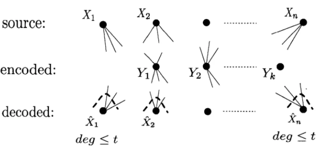
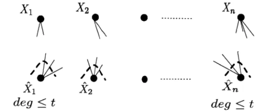
The problem of locally decodable source coding (LDSC) is studied in this chapter where

a source sequence z1, x 2, ... , taking values from the source alphabet X, is mapped into a

sequence Y1, Y2, ... of symbols taking values in the compression alphabet Y. These symbols are then used to produce the reproduction sequence Y1, x2, ... in the alphabet X. The rate

of the source coding is defined as the ratio of the length of the output sequence to the input sequence (normalized by the size of alphabets). The decoding scheme is called t-local

if, for any i = 1, 2, ..., _{the reproduced symbol, i only depends on t of yi, Y2,} ... (t is

called the number of queries). In conventional source coding,

in

depends on

Yk

in an arbitrary manner. In this work, we characterize the source coding rate for the setting in which the decoder is constrained to ask only t queries to reproduce any reproduction source coordinate , i.e., fi. Figure 3-1 demonstrate the problem formulation. As it shows, any yj is an arbitrary function of x1, x2, ... and any

s,

is a function of only t of Y1, Y2, ...

This problem appears in many applications in distributed data management. For in-stance, assume a given source is stored in some storage cells. Since writing on data storage cells is generally costly, we use source coding to decrease the number of cells used. If we wish to recover a part of the original source (in our case one coordinate of the source sequence) we may need to read the entire encoded data on all data storage cells. Therefore, we need to query all the cells and then decode the coordinate of the source that we wanted to recover. However, we know that reading from the storage cells is generally costly, so we wish to read as few cells as possible. Clearly, there is a trade off between the number

(26)

x1 X2 Xn

source:

\

-encoded:

_YX

_Y2 _Yk

decoded:

«

---x1

X2 Xn deg <t deg t

Figure 3-1: Locally Decodable Source Coding

of used storage cells to store the entire original source (rate) and the number of cells we need to access in order to recover a coordinate of the original source sequence (locality, t). Characterizing this trade-off is one of our goals.

In another example, assume that we encode a source and then store it on some data storage cells. We want to reveal the information about one coordinate of the source to some party, but, we do not want to reveal the information about the entire source symbols.

If we use a conventional source coding, we may have to reveal all the encoded data. Thus,

a honest but curious party may have access to the entire original source sequence. On the other hand, in LDSC we provide only a small part of the encoded data, so the party can only recover the desired part of original source symbols without capability of extracting the other symbols.

3.1 Lossless Locally Decodable Source Coding

In this section, we study lossless source coding in the presence of local decoders. We formally define LDSC and study its rate.

3.1.1 LDSC

A local decoder is a decoder that only asks a few number of queries to decode any

(27)

as follows. A lossless LDSC is defined as a pair consisting of an encoder,

f,

and a decoder,

g, where,

f

: X" - {0, 1}k and g : {0, I}k _ X". The decoder is called local if each

coordinate of the output is affected by a bounded number of input coordinates. Formally, Let g,, for a E {1, ..., n}, be the a-th component of the decoding function. Assume ga

de-pends on yk only through the vector Y = {Y

j

E A/:x} for some Af c {1, ... , k},

meaning that

For any yk and y'k, ge(yk) = ga(y'k) if -'".

For any given t, a decoder is called t-local if |Nf<l <t for any a

C

{1, ... , n}.

Definition 4. An (n, k, t, c)-LDSC is a pair consisting of an encoder

f

X" {0, 1}k

and a t-local decoder g : {0, I}k 1 X", such that

jp[gyf (X"))

#

X"] < e (3.1)

Using a similar notation to that of [21 ], let

k c*(n, c, t) A min{k : 3 (n, k, e, t) - LDSC}. (3.2) Where the subscript ld stands for local decoder The best rate of local code for a given n, t and E, is given by

Skz* (n, c, t)

RId(n, e, t) = . (3.3)

Also let

Rld(E, t) A lim sup Ri(n, E, t). (3.4)

n-+oo

We define the rate as

R (t) wlim Rad(E _E-+0 t). (3.5)

(28)

an (n, k, e, t) - LDSC code with deterministic encoder and decoder

Proof: Let M and N be two random variables, and consider randomized encoder and

decoder f(M) and g(N), respectively. Equation (3.1) then becomes

P[g(f(X", M), N) # X"] = E[IP[g(f(X", M), N) # X"]|M, N] < e.

Since the probability in equation (3.1) is less than or equal to E, then there exist m, n such

that

IP[g(f (X", M), N)

#

XIlM = m, N = n] < c,

implying that f(m) and g(n) are our desired sort of encoder and decoder, respectively, and

the proof is complete. D

Note 3. Using Lemma 1, in the rest of the text, we assume the encoder and decoder are

deterministic.

3.1.2 Average LDSC

Instead of assuming the number of queries to recover any Xi is bounded, consider the

case where the average number of queries asked to recover all the Xi s is bounded. We

term this Average Locally Decodable Source Coding (ALDSC). The formal definition is the

following.

Definition 5. For any given t, a decoder is called t -average local if - E _1 |X I t. An

(n, k, t, c)-ALDSC is a pair consisting of an encoder

f

X" -+ {O, I}k and a t- average

local decoder; g : {0, I}k ₊X, such that

jP[gyf(X")) # X"] < e

Similarly, define

(29)

where the subscript, ald, stands for average local decoder. The best rate of a ALDSC for a

given n, t and c, is given by

Raid (n,c, t) al i(n , E I

n

Also, define

Rald(E,t) A limsupRad(n,,Et).

n-*oo

We define the rate as

Raid(t) A lim Rald(E,t).

The following result establishes a relation between Rld(t) and Raid(t).

Proposition 1. For any 0 < A < 1, we have k* (n, c, t) > k*ld(An, k, , t).

Proof: The proof follows from sorting the number queries for all of the source symbols

and then selecting the first A fraction of them. Let (n, k, t, E) be an ALDSC. Let tj denote

|NIl for 1 < i < n. Without loss of generality, assume ti 5 t2 ... K t. We have

1

En

tj < t (for the sake of presentation, without loss of generality, we drop ceiling and

floor). Therefore, we get tAn < 1. The corresponding decoder and encoder introduces a

(An, k, tA, ) - LDSC. Hence,

{k 1 (n, k, c, t) - ALDSC} c { k | E(An, k, e, ) LDSC} 1 - A

t

->kald(n, , It) > kz* (An, k, c, )

1 -A

The proof is complete.

Corollary 1. For any 0 < A < 1, we have ARId( t A) < Rad(t).

Proof: Using Proposition 1,

t k*(An, c, ) k, k, t)

ARld(- ) = A. ld ld = Rald(t),

(30)

which concludes the proof. D This corollary states that, once we have a lower bound on the rate of LDSC, we obtain a lower bound on the rate of ALDSC. Implying that we would not gain much, by using

ALDSC instead of LDSC. We shall quantify this notion in next sections.

3.1.3 Linear Encoder

Source coding with a linear encoder and local decoder is the subject of this section. We focus on binary sources where X = {0, 1}. We show that, for a linear encoder, the rate

of LDSC is one instead of the entropy rate, implying no compression is possible. Before proving this fact, we introduce the influence matrix of an encoder.

Definition 6. Let

f

: {0, 1} -+ {0, 1} be a Boolean function defined on {0, 1}'. The influence of Xi (the ith component of

f

) on

f

is defined as

Infi(f) P[f(x + ei) # f(x)]. (3.6)

An encoder

f

: X" + {0, I}k can be treated as a collection of k Boolean functions on

{O, 1}". If we denote the jth function by

f

_{3, then f (x)}= (f1(x), ..., fk(x)). The influence

matrix of the encoder

f

: X" - {O, I}k is an n x k, matrix, A, defined as Aij = Infi (fj).

Note that if a function is linear then the influence matrix in the same as the generating matrix.

We illustrate a relation between a function Influence and its ability to decode a particular bit by an example.

Example 1. In this example, we show that two functions f1 and f2 may recover X ₁, while

having almost zero information about X 1. Let f1 = X1 +... + Xn, and f2 = X2 +-- ... + Xn,

where the summation is in F2. Here, we have perfect recovery by X1 = f1 + f2. We have

Infi(fi) = 1 while I(Xi;

fi)

= h(I(1 - (1 - 2p)"n) - h(!(1 - (1 - 2p)"-1) which is very close to zero for large n. On the other hand, Inf 1(f2) = 0 and also I(X1; f2) = 0.

(31)

Next, we prove a converse bound on the a rate of LDSC with linear encoding. In order to prove the theorem, we use the following lemma.

Lemma 2. Let F' be a vector space over F2. Let Px = Bern(p) and define a probability

measure over F' according to P". If U is a k- dimensional sub-space of FY, we have

(max{p, 1 - p})"~k ;> P[U] > (min{p, 1 - p})"-k.

Proof: We first prove the lower bound. Define E = {v E VI H(v) = 1}, where H(v)

denotes the hamming distance of v. Since the dimension of U is k, there is E' a subset of

E with n - k elements such that

U T U' = Fn

U n U'= {O},

where U' = span{E'} and D denotes the direct sum of two sub spaces. For each u' E U'

define Uu, = U + u'. It is clear thatUu/

n

Uu, 0 for u'

#

u'. Next, we shall bound P(Uu,). Suppose H(u') = r, then we have:

P[U]= E P[U]= EP[U+U']

U(EU.i 2U

(

max{p, 1 - p}Jmin{p, 1 - } r

ru( min{p, 1 - p} r

I max{p, 1 - p}J

Since Uns are disjoint and for each u' E U', we have H(u') < n - k and the following

equation holds

1 = P[F"] = P[UrEU, U,] = IP[UU/]

n-kn - k maxrp, - p - PU] ( r _{minfp, 1 - p}} max{p, 1 - p} n-k min{p, 1 - p} = P (min~p, 1 - p}I P[u]

=P[U] 1I

(3.7) < P[U] max~p, 1 - p} r U/EU/ (minifp, 1 - p} )

(32)

Changing the second line of (3.7), the upper bound is proved similarly. El

Theorem 7. Assume X has a Bern(p) distribution and (n, k, c, t) is a LDSC for this source with a linear encoder If 6 < (min{p, 1 - p})t, then k > n.

Proof: Let G be the corresponding influence matrix of the encoder. The encoding is

then as following

x -+ xG.

Since the encoder is linear, the entries of the influence matrix are either 0 or 1, meaning

G E P G9". G is a mapping from {0, 1} to {0, 1}k. Without loss of generality, assume that X1 is recovered by Y1, ... , Y and the decoder maps 0' to X1 = 0. Consider the induced

linear mapping7r : X" Y, we have dim(ker(G)) > n - t. Note that on G ker(7r). If

there exists X" E ker(7r) such that x₁₌_{1, then half of the vectors in ker(7) have x}₁ ₌₀

and half of them have x1 = 1. Since the decoder maps 0 to Xi = 0, then the vectors

in ker(7r) with x1 = 1 are erroneous . Eliminate the first coordinate and consider all the

vectors in ker(7r) such that x1 = 1, they will form a subspace of dimension at least n - t -1

is a paces of dimension n - 1. Therefore using Lemma 2

P[in

#$

X"] > P[I

#

X1] > P[S] > (min{p, 1 - p})"--1-(n-t-1) = (min{p, 1 - p})'.

Which is a contradiction.

Hence, for any x" E ker(7r), xi = 0. This means that, if we look at the sub-matrix of G

of dimension n x t consisting of the first t columns, the first row is not in the span of the rest of rows. This implies that, in the matrix G, the first row is not in the span of the rest of rows. If we apply the same argument for any Xi, we conclude that the rows of the matrix

G are independent, resulting in k > n. E

Corollary 2. Using linear encoder; for any t, we have Rld(t) = 1. Moreover; by using

Proposition 1, we have Raid(t) = 1.

Proof: It directly follows from Theorem 7 and Corollary 1.

(33)

the rate, which is entropy, meaning that we can not compress data, expecting to recover it locally.

Note that, Theorem 7 also proves that using a linear encoder and local decoder, we can only have lossless (with zero error) codes.

3.1.4 Linear Decoder

In this section, we assume that the decoder is local and linear. We show that, for a linear decoder, even without locality constraint, the rate of compression is 1. This implies that, if the decoder is linear, then no compression is possible.

Theorem 8. Let X have Bern (p) distribution. Assume the decoder is linear. We have

log(1 - e

k*c(n, e) > n - log( - (3.8)

Sc _{log (maxfp, 1 - p})} Proof:

Consider a (n, k, E)- SC. Assume e1, ... , ek are the canonical basis of {0, 1}k. Decoder

can only recover Span{g(ei), ..., g(ek)} and we have error for all other inputs. Thus, using

Lemma 2

P[g(f(X"))

#

X"] > 1 - IP[Span{g(ei), ... , g(ek)}] ; 1 - (max{p, 1 - p})"-k

we also know P[g(f(X"))

#

X"] < E. Therefore,

k > n log(1 - e)

- log max{p, 1 - p}

Taking the minimum over all choices of codes, we get

k*c(n, e) ;> n - o~ -E

log (max{p, 1 - p})' and the proof is complete.

Let X be a Bern(p) source and f : X -+ {0, I}k and g : {0, I}k '-+ X" be the general

(34)

employ linear decoding, the rate of compression is always one, instead of entropy rate. Therefore, for any t-local decoder we have

Rld(t) = 1.

Moreover, using Corollary 1 for a linear decoder, we obtain

RaId(t) 1.

3.1.5 General Encoder-Decoder

In previous sections, we showed that assuming a linear encoder or linear encoder the rate of LDSC is 1. We study the same problem for a general encoder-decoder. First, by using an example, we show the existence of good non-linear encoders with local decoder.

Example 2. Consider the following

f

:

fo = X1 or X 2 or ... or X, fi = Xi or (X1 or ... X _1 or Xi+1 or ... or Xn + 1).

The recovery is as

Xi = fo and

fi.

In this example we have zero error and k = n + 1. This shows the existence of completely non-linear codes.

The following theorem focuses on the special case of t = 2. Without loss of generality, we assume p < 1

Theorem 9. Let X be a Bern (p) source and f : X" ' {0, 1}k and g : {0, 1}k '-* X" be a

general encoder and t-local decoder, respectively. Also assume a (n, k, c, t)-LDSC for this source. For t = 2, if E < p2, then k > n.

Proof: We prove this by contradiction. For the sake of contradiction, assume n > k,

we show that c > p2_{, which is a contradiction.}

The claim is that if the code can recover X 1 _{(i.i.d Bern(p)) with a local map from} 1

(35)

on a set with probability p(k), then p(k) < 1 - p2. Note that this is enough to prove the

theorem because e = 1 - p(k) > p2

By induction on k, we show that p(k) < 1 - p2_. _{It can be shown that p(l) < 1}

-p2. Let

p(k - 1) < 1 - p2. Assume X₁ is recovered by Y and Y₂. Without loss of generality,

assume that g1 (0, 0) = 0, where for any 1 < i < n, gi is a mapping, with two inputs, that

reproduces Xi. Here are the all possible cases:

1. g1(0, 1) = 0. In this case, if we consider the induced map from Y2 to X2+1 by

replacing 0 with Y in all the mappings that use Y as one of their inputs, we end up with a local mapping on a set with maximum probability of p(k - 1). Similarly, since 91(1, 1) = gi(1, 0) = 1, if we replace 1 with Y, we get another local mapping on a set

with maximum probability p(k - 1). Therefore, p(k) 5 p.p(k -1) + 1 - p.p(k -1) =

p(k - 1) <1 - p2

.

2. g1 (1, 0) = 0. In this case, replace 0 with Y2 and construct a mapping from Y1, Y2 to

X2+ 1_{. Similarly, it can be shown that p(k) < 1}_- _p2_.

3. g1(1, 1) = 0. In this case, replace Y by Y2 in all the mappings that use Y as one of

their inputs. Similarly, we obtain p(k) < 1 - p2.

4. g(1, 0) = g(0, 1) = g1(1, 1) = 1. In this case, gi(Y, Y2) = Yi1. 2. This case

requires more details which will follows.

We call Y1.Y2, Yi-Y2, Y1.Y2, and Yi.Y 2 a product form. The discussion which we provided

before shows that if only one of the k

+

1 mappings is not of the product form, then the

above argument proves p(k) < 1 - p2. Now, assume all the mappings are in the product

form. If Y is once used as Xi= Y.Y and once as Xi2 = Yi.Yk, then X1 = X2 = 1

cannot be recovered. Implying p(k) < 1 - p2 < 1 - p2 (p < 1). Therefore, without loss of

generality, we assume that all the mapping functions are of the form Y.Y.

There are k + 1 mappings, so the number of arguments of all these mappings is 2(k +

1). Also, note that there are k Y's. Thus, three mappings can be found as Xil = YY, Xi2 = Y Yk, and X., = YY. If Xt, = 1, then we can find a mapping from Y', Y+1

(36)

Xi2 = Xi, = 1 is not possible to recover. Therefore, p(k) < p.p(k - 1) + p.p2 ₁ _{_}_p2_.

The proof is complete for t = 2. 0 Corollary 3. Let X be a Bern(p) source. For t = 2, Rld(t) = 1.

Proof: It directly follows from Theorem 9.

Also, for ALDSC we obtain the following.

Corollary 4. Let X be a Bernoulli (p) source. For t = 2, Rald(t) = 1.

Proof: It follows from Theorem 9 and Corollary 1. D Considering the bipartite graph describing the relation between input and output of a gen-eral decoder, one way to gengen-eralize this proof to t > 3 is to find a small number of encoded coordinates that are connected to a small number of recovered source coordinates. The fol-lowing section discusses this idea. We have the folfol-lowing conjecture for any given t > 2: Let X be a Bern(p) source and

f

: X" ' {0, 1} and g : {0, 1}k '-* Xn be a general

encoder and t-local decoder. For any t, we have RId(t) = 1. As a result of Corollary 1, Rald(t) = 1 follows.

3.1.6 On the Bounded Degree Bipartite Graph

In previous section, in the case of t = 2, we found two Xi's which are connected to only two of Y 's. Then we considered all the possibilities for this sub-mapping and then did induction to prove Theorem 9. If we can find a subset of the Xi's with size s which are connected to a small number of Y's such as s + 0(1), then we would follow the same approach as of the proof of Theorem 9. The following result rules out this approach. Let G(U, V, E) be a bipartite graph, where U and V are two set of nodes connected with the edges from E.

Definition 7. We call a bipartite graph G(U, V, E) a t - regular bipartite graph if any node in V has a degree equal to t. Moreover let the set G(n, m, t) = _{{G(U, V, E) t} -regular such that

|U|

= m,

|V|

= n}.

For a given subset of the nodes V such as I, let N(I) denote the neighbors of the nodes in I.

(37)

Definition 8. For any given 1, let

N(1, n, m, t) = max min N(I).

GEG(n,m,t) 1:1I=1

In order to obtain insight about N(l, n, m, t), consider the following example.

Example 3. If m > nt, then N(l, n, m,t) = lt and the graph that achieves this is the one for which all nodes in V are connected to disjoint set of t nodes of U. If m is very small

relative to n, then N(l, n, m, t) is below it.

We are interested in the case where m = n - 1. The question we try to answer is the

following: for a given t and 1, what is N(l, n, n - 1, t), for large enough n. The following

theorem shows that the number of neighbors of a set of size 1 is growing at least linearly with 1.

Theorem 10. For any given t, 6 and 1, there exists no(t, 1, 6) such that, for n > no(t, 1, 6)

N(1, n, n - 1, t) ;> (t - 1 - J)1.

Therefore, N(l, n, n - 1, t) grows not slower than linearly with 1, for a given t.

Proof: Let the set X = {1, ..., n - 1} denote the nodes in U. Let A,..., Ak be k

sub-sets of X, each of them with t elements corresponding to the neighbors of the v in X, where v

c

V. Also, assume that the union of any 1 of these subsets has at least (t - 1 - 6)l

many elements. We must show that, for large n, there exists a collection of size n of these subsets, i.e. k can be equal to or larger than n. We use a probabilistic approach to show this. Assume that the subsets are chosen uniformly from X. Let 1{| U'_1 AiI < (t - 1 - 6)l}

be the indication function which is one if its argument holds and is zero otherwise. Now, consider the following expectation for a given k, n, t, 1:

E[ 1{|I U1._1 Ai,|I < (t - 1 - J)1}].

If this quantity is less than one, then for the given k, n, t, 1 there exists a bipartite graph in

(38)

more than or equal to (t - 1 - _{()l node. Thus, in order to complete the proof, we show that}

there exists no(t, 1, 6) for which, if n > no(t, ,), then the expectation becomes less than

one for k = n.

We have

E 1{I u1_1 Aij < (t -1 -6)l}] = P[ Ui 1 AiI < (t -1-6)1].

Let N(t, 1) denote the number of different ways in which one can choose 1 subsets of a set

with (t - 1 - 6)l elements, each of them having t elements. We obtain

n-1 P

(|U11

Ai| < (t - 1 -6)] = 1 N(t, 1). Hence, Ef 1{ U1 Ai, < (t - 1 - 6)}= = N(t, l) (n - 1)(t-1-6)1 /n(n - 1)(t-1-6 < k' _ N(t) 1) < (t!)l N(t, 1) (n-1-t)t (n -1- t)t

Comparing the exponent of n in the numerator and denumerator, there exists no(t, 1, 6)

(some number which depends on t, 1, and 6) with the property given in the theorem. El

3.1.7 Scaling Number of Queries

As we mentioned before, the number of queries, t can be a growing function of n. In the conventional source coding ( not necessarily local) t(n) is a linear function of n. Therefore, the regime of our interest is the one where t(n) grows sub linearly with n. In order to establish the results on LDSC with scaling number of queries, we need the following results on the error exponent of source coding to establish an achievability bound on the rate. This approach is motivated by the achievability bound given in reference [15].

(39)

source encoding with rate R, we have:

For any c > 0, 3 Ke such that for any n > 0 there exists an encoding-decoding pair

f"

and g such that

P[gn(fn(X"))

#

X] & e-n(E(R)-)

Where

E*(R) min D(Q||P).

Q:H(Q)>R

Moreover this bound is asymptotically tight.

Now, consider the following construction of an encoder-decoder for a sequence of length n of the source Bern(p):

Let the rate R be equal to (1 + 6)H(X). Let X" be a sequence of source symbols. Di-vide this sequence into blocks of length t(n) and apply the encoder-decoder pair found by Theorem 11 to each block separately. Form an encoder-decoder for X" by cocatenating these n (for the sake of presentation, without loss of generality, we drop ceiling and floor in this analysis) pairs of encoder-decoder. We now analyze the error of the concatenated source coding. Using a union bound we obtain

p[Xn <t n) tn

P["#X") = p[Utd"){ X' X }]~n P[ZA") # Xt3].

Using, (3.9) for any c, we obtain

P[Xn

#

X"] ] K 2-t(n)(Eg(R)-e)

t(n)

Since R > H(X), E*(R) =A > 0. Thus, we have

lp[.n f Xn] < n K62-4)-) -t (n)

Choose c < A and denote A - E by F. We want to see for which choices of t(n), this bound goes to zero. This happens when

lim Ft(n) - log = 00

(40)

resulting in

t(n) > Clog n,

for some constant C. Therefore, we have the following result.

Proposition 2. Let X be a Bern (p) source and

f

: X" + {O, I}k and g : {O, I}k _ X,

be an encoder and t(n)-local decoder For any e and R > H(X), there exists a C and no such that for n > no, there exist a (n, nR, C log n, c)-LDSC.

This theorem states that with number of queries (log n) that is small relative to n, the rate of LDSC approaches the optimal rate h(p).

The same results also holds for linear codes. In particular, we use the following results.

Theorem 12. ([5]) For a given source with probability measure Px, n, and k there exists a linear encoder;

f

: X" X- k and and a decoder such that

P[Xn - X"] 2-n((R-H(P))-2x2 log n1)

Using this theorem we get the following result for linear encoders and local decoders.

Corollary 5. Let X be a Bern(p) source and let

f

: X" H

{0,

I}k and g : {O, I}k + X"

be a linear encoder and t(n)-local decoder; respectively. For any c > 0 and R > H(X), there exists a C and no such that for n > no there exist a (n, nR, C log n, e)-LDSC.

3.2 Lossy Locally Decodable Source Coding

In this section, Locally Decodable Lossy source Coding (LDLSC) is studied. First, we formally define the problem.

Consider a separable distortion metric defined as d(X",

Z")

=

Z

1 d(Xi,

Zi).

Definition 9. A (n, k, d, t)-LDLSC is a pair consisting of an encoder

f

: X" F yk and a

decoder g : yk + X" , where the decoder is t-local. The average distortion is bounded,

E[d(X",Ig(f (X")))] < d.

Let

(41)

where the subscript ,ld, stands for local decoder; also

k*(n, d, t )

Rld(d, t) Alim sup .(.1

n-oo n

Note 4. We assume a binary source, F = F2 with d(X, X) = 1{X

#

X}. In this case, we have

E[d(X", g(f (X")))] =

i

P[Xi f

Zi]

d,

i=1

which is the same as assuming the bit error rate is bounded (relative to the block error rate in the definition of LDSC).

3.2.1 Scaling number of queries

In this section, we consider the scaling of number of queries. Therefore, let t(n) shows the number of queries. The following is an upper bound on the rate for scaling number of queries.

Theorem 13. For a Bernoulli(p) source, a distortion level d, and any increasing number of queries t(n)

log t(n) log t(ni)

RId(n, d, t(n)) < h(p) - h(d) + t(n) +o( ) (3.12)

t(m) t(n)

Proof: Recall the finite block length results on source coding ([27]) thereof for a

Bern(p) source, and distortion level d, there exists a code such that

Ric(n, d) < h(p) - h(d) + + o( ). (3.13)

n n

Now, divide the sequence X" into ' blocks of length t(n). Apply the encoder-decoder obtained from (3.13) to each block. Concatenate these n pairs to obtain an encoder-decoder for X". The average distortion of the overall code is also bounded by d, and its rate is bounded by

(42)

which shows the theorem. D Theorem 13 shows that, for any number of queries t(n), if lima, t(n) = o, then there exists (n, k, D, t(n))-LDLSC such that k < n(h(p) - h(D)) + o(n). Note that

without loss of generality, we dropped ceiling and floor in the analysis.

Corollary 6. For the special case t(n) = t log n, we have

Rld(n, d, t log n) < h(p) - h(d) + log log ( (3.14) t log n t log n

Proof: The result of Theorem 13, for t(n) = t log n. D Patrascu ([20]) studies the problem of storage of bits with local recovery of bits (with the same definition of locality we use here). Those results are based on a generic transformation of augmented B-trees to succinct data structures. He shows that

Theorem 14 ([20]). Consider an array of length nfrom alphabet X. We can represent this array with a number of bits

O(|X log n) + nH + ( , + O(ns/4 _{log ns/}4_), _(3.15)

(

)t

supporting single bit recovery in t log n queries, where H denotes the empirical entropy (the entropy of the empirical distribution). Moreover; we can represent a binary sequence of length u, with n ones, using

log

+

t)( + O(U3/4 _log 3/4) _(3.16)

bits, for which a decoder exists querying only t log u bits. Note that the encoder/decoder knows n and u beforehand.

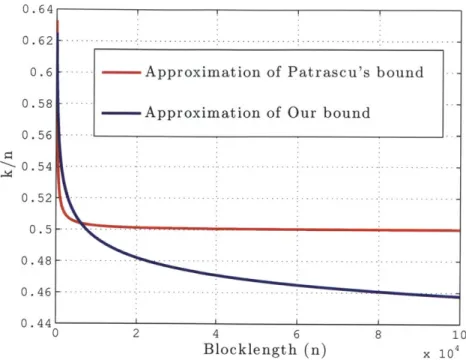
Reference [20] essentially studies the case of t(n) = t log n. We now compare the bound given in corollary 6 with the bound suggested by Theorem 14.

Using Theorem 14 and identity log

(")

= nh(p) + O(log n), for any d, we obtain

Locally decodable source coding