Out-of-Core Build of a Topological Data Structure from Polygon Soup
Sara McMains Joseph M. Hellerstein Carlo H. S´equinComputer Science Department University of California, Berkeley∗
Abstract
Many solid modeling applications require information not only about the geometry of an object but also about its topology. Most interchange formats do not provide this information, which the ap-plication must then derive as it builds its own topological data struc-ture from unordered, “polygon soup” input. For very large data sets, the topological data structure itself can be bigger than core mem-ory, so that a naive algorithm for building it that doesn’t take virtual memory access patterns into account can become prohibitively slow due to thrashing. In this paper, we describe a new out-of-core al-gorithm that can build a topological data structure efficiently from very large data sets, improving performance by two orders of mag-nitude over a naive approach.
1
Introduction
The topology of a boundary representation (b-rep) – the connectiv-ity of its faces, edges, and vertices – is as important as its geometry for many applications. This connectivity information can be used for operations ranging from computing offset surfaces, to calcu-lating vertex normals for smooth shading, to mesh simplification. Many data exchange formats that describe b-reps only specify the geometry of the boundary, leaving it up to the application to dis-cover the connectivity. Such an unordered b-rep describing faceted geometry is colloquially referred to as “polygon soup.”
For a small model that fits easily in memory, it is efficient for the application to build up its own topological data structure by in-crementally updating it for each new polygon in the input. This naive approach is disastrous, however, for very large data sets, such as those produced from laser-range finder scanned 3-D input (see the Digital Michelangelo Project [15] for examples of enormous geometric data sets containing as many as two billion polygons de-scribing a single object). When our data structures no longer fit in core memory, we need to use different techniques to avoid access-ing virtual memory randomly.
We introduce a new out-of-core algorithm that can build a topo-logical data structure efficiently even from very large, unorganized data sets. Our implementation takes “triangle soup” in STL format [1] as input. This is the de facto standard interchange format for solid freeform fabrication, a class of technologies used to manufac-ture complex 3D geometries by building them up in layers [4]. Our algorithm builds a Loop Edge-use Data Structure (LEDS) represen-tation, a topological data structure closely related to Weiler’s radial
∗{sara|jmh|sequin}@cs.berkeley.edu
edge structure [26]. The principles of the algorithm, however, are applicable with any faceted input and any topological data structure. For comparison, we also describe the design and implementation of an in-memory algorithm that builds the LEDS efficiently from small STL files, but thrashes when input files are large compared to available memory.
2
Previous Work
2.1 Topological Data Structures
The data structure that we build is closely related to Weiler’s radial edge structure [26]. The radial edge structure is a generalization of Baumgart’s winged edge data structure [3] to non-manifold geome-try. These data structures allow us to answer questions about topo-logical adjacency relationships, e.g. the faces incident to an edge, often either in constant time or in time proportional to the size of the output set. Weiler’s data structure also records the radial order-ing of faces around non-manifold edges (hence its name). Another important concept from Weiler’s work is the distinction between an abstract, unoriented geometric element, such as an edge, and an ori-ented use of that element, such as a directed edge-use that describes part of the boundary of a face. Other variations on these data struc-tures include M¨antyl¨a’s half-edge data structure [16], which is lim-ited to 2-manifolds, Rock and Wozny’s topological data structure for STL [19], also limited to 2-manifolds, and the data structure that ACIS modelers build and exchange in .sat files [21]. Another important non-manifold representation forms the basis for the Noo-dles system developed by Gursoz, et al. [12]. Guibas and Stolfi’s quad-edge data structure [11] is limited to 2-manifolds but can si-multaneously represent the topology of an object and its dual.
2.2 Out-of-Core Algorithms
Numerous out-of-core techniques have been developed for other geometric applications. In the graphics domain, these applica-tions include large building walk-throughs, radiosity, and ray trac-ing [9, 23, 18]. In the visualization domain, several researchers have addressed out-of-core isosurface extraction [6, 5, 22, 2]; oth-ers have looked at visualization of terrain and computational fluid dynamics, including streamlines on meshes [8, 7, 24].
Although our input is geometric, the problem of updating con-nectivity pointers in a topological data structure actually has a closer analogy in building object oriented databases (OODBs). In these databases, the presence of inverse relationships means that inserting one object in the database requires the system to update all of its inverses, which must point back to it, as well. Wiener and Naughton have proposed a solution for efficient bulk-loading of OODBs [27] that provides the inspiration for our approach. The major insight in their work was that the inverse relationship up-dates can be reformulated as analogues of database “join” opera-tions. These can be resolved efficiently for very large data sets us-ing “partitioned hash join” algorithms [10]. These algorithms build, one at a time, memory-sized pieces of a larger hash table, in order to avoid memory thrashing.
3
Data Representations
Our algorithm reads input in the STL format, a boundary represen-tation that consists of a simple list of triangular facets. The vertex coordinates are specified explicitly for each triangle in which the vertex appears. The vertices are enumerated in counter clockwise order as seen from the exterior of the part. In addition, for each triangle, a redundant surface normal that points to the exterior of the part is specified. An example of an STL triangle specification is shown in Figure 1. facet normal 0.319565 -0.175219 -0.931222 outer loop vertex 2.410370 -7.779990 -8.411049 vertex 2.407310 -9.749799 -8.050910 vertex 2.229340 -9.927230 -8.628259 endloop endfacet Figure 1: An STL triangle.
Our algorithm constructs a Loop Edge-use Data Structure (LEDS) describing the topology (connectivity) of the STL input. LEDS supports all bounded, rigid solids, or r-sets [25], including not only 2-manifold solids but also the subset of non-manifold ge-ometry that corresponds to physically realizable solid objects, such as the one pictured in Figure 2. On such objects, the neighborhood of each point on the boundary is topologically equivalent ton2D disks,n ≥1, and each edge in the b-rep is used an equal number of times in both directions.
Figure 2: A non-manifold part that is a valid solid.
In the LEDS, we have stripped away some of the overhead, which we don’t require for solid freeform fabrication applications, from Weiler’s radial edge structure. Weiler separates undirected loops or faces from directed face-uses and loop-uses, allowing the same face to be referenced from both sides where it forms a mem-brane between cells, for example. We only represent the actual directed face-uses and loop-uses, since a single face or loop is un-likely to be used more than once in solid freeform fabrication file descriptions. For simplicity, we will refer to face-uses and loop-uses as faces and loops in the rest of this paper.
Each face (see Table 1) is defined by one counter-clockwise, outer loop and a (possibly empty) list of clockwise, inner hole loops. For triangulated STL input, we will have no inner hole loops in the input geometry. Loops are represented implicitly in the LEDS: in a face, we store a loop simply as a pointer to an arbi-trarily chosen edge-use in that loop. Each edge-use stores a pointer to the next edge-use in the loop; we follow these pointers to traverse the loop.
FACE
EDGE USE * First Outer Loop Edge Use
List<EDGE USE *> Inner Loop List
Table 1: The connectivity data stored with a LEDS face.
Each edge-use in the loop points back to the face whose bound-ary it helps to define (see Table 2). To make edge-uses compact, we
store only one vertex pointer with each edge-use, a pointer to the root vertex (the vertex from which the edge-use is directed away). The vertex on the other end can be found by following the pointer to the next edge-use in the loop and getting its root vertex. While we represent each edge-use explicitly, the abstract, undirected edges are represented implicitly by circular lists of edge-uses sharing the same endpoints, linked by “sibling edge-use” pointers stored with each edge-use.
The LEDS also records a separate edge list that contains point-ers to these implicit edges, storing each as a pointer to one arbitrar-ily chosen edge-use in the linked list of sibling edge-uses for the edge. This allows an application to iterate through all the edges ef-ficiently, without visiting each edge-use. The LEDS also stores lists of its faces, vertices, and edge-uses to support adding and deleting geometry after the initial input is read.
EDGE-USE
FACE * Face
VERTEX * Root Vertex
EDGE USE * Next In Loop Edge Use EDGE USE * Sibling Edge Use EDGE USE * Next Vertex Edge Use
Table 2: The connectivity data stored with a LEDS edge-use.
An important feature of this data structure is constant space stor-age for each vertex and for each edge-use. Rather than storing a variable length list of all of the edge-uses incident to a vertex with the vertex, we chain together all of the vertex’s edge-uses into a cir-cular linked list (in arbitrary order) via the Next Vertex Edge Use field in the edge-uses. The vertex contains a pointer to any one of the edge-uses in this circular list (the First Vertex Edge Use field in Table 3). The combination of these pointers allows us to iterate through all of the vertex’s edge-uses, even at non-manifold vertices.
VERTEX
float[4] Coordinate
EDGE USE * First Vertex Edge Use
Table 3: The position and connectivity data stored with a LEDS
vertex.
For representing STL input, the space usage for each face is also constant since the faces have no inner hole loops. Constant space storage is important for allocating memory efficiently; it allows us to pre-allocate storage in arrays.
4
Hashing
To build a LEDS from unorganized STL input, we use hash tables in both our in-memory algorithm and our out-of-core algorithm. Since STL doesn’t provide vertex identifiers, we use a vertex hash table to match up coincident vertex coordinates. To determine the edge connectivity, we use an edge hash table to match up edge-uses with their coincident siblings.
For the vertex hash tables, we use thex,y,zcoordinate triple as the input to the hash function. In addition to the input value (the hash key), we store (as the hash data) a pointer to the LEDS ver-tex for the in-memory algorithm; for the out-of-core algorithm, we store the vertex’s index in the final LEDS vertex array (as explained in section 7). The pointers and indices are both 32 bits; thus both algorithms’ vertex hash table entries are the same size.
In the edge hash tables, in order to match an edge-use with its sibling(s) which may be oriented in the opposite direction, we want the hash function to return the same value regardless of the order of
the edge-use’s endpoints. We accomplish this by ordering the end-points lexicographically, and use this ordered pair as the input key to our hash function, which also allows us to use a standard equality check. We don’t use the coordinate triples of the endpoints, how-ever, but rather the endpoints’ data values from the hash table, since these are one third the size. Again, the hash table keys are the same size for both algorithms, though they are different keys. For the in-memory algorithm, the edge hash table will record a pointer to a single edge-use in its data field, but for the out-of-core algorithm the edge hash table will record up to two array indices of LEDS edge-uses in its data field, as described in the sections on the re-spective algorithms. Thus the in-memory algorithm’s edge hash table entries will be smaller.
We chose our hash functions both to be quick to compute and to minimize collisions in the hash table. Integer computations are faster than floating point computations, so our hash function treats the 32 bits that represent each normalized floating point coordinate as a 32 bit integer. As part of satisfying the second goal of mini-mizing collisions, we use all three coordinates and both endpoints as input to our hash function, so that we won’t get additional vertex collisions for files that have many vertices with the same height, for example, or additional edge-use collisions for files with vertices of high valence. We can merely add the two values together in the case of edge-use hashing because we want edge-uses in either direction to hash to the same value. For vertices, however, we mul-tiply the three values by different numbers before adding them up to avoid collisions between permutations of the same coordinates, which could be an issue for symmetrical parts. We use identical hash functions for the in-memory and out-of-core algorithms.
We address collisions in our hash tables by using open ing and double hashing to find an empty slot. (Open address-ing means that if an input value hashes to a position that has al-ready been used for another value, rather than “chaining” together a linked list of multiple entries for that position, we follow a probe sequence until we find an empty slot. Double hashing is a tech-nique for choosing this probe sequence using a second hash func-tion to choose an offset value. See [14].) Once a hash table is very full, its performance degrades drastically, as we must search a longer and longer probe sequence to find an empty slot. When a hash table is filled to 80% capacity, the total number of misses will be roughly equal to the total number of hits; at this time we rehash in a new hash table that is twice the size (“rounded” up to the next prime number, of course) to improve the hit rate. In gen-eral, a larger hash table will give better performance at the expense of using more memory. We feel that rehashing at 80% full is a reasonable time/space tradeoff.
5
Test Files and Platform
To examine the effects of file size on performance, we timed the performance of our algorithm implementations on a series of files that approximate the same ideal geometry. Our canonical “knot” test part, shown in Figure 3, is output from S´equin’s sculpture gen-erator [20]. We varied the fineness of the tesselation to produce different sized files containing 10,000 to 1,000,000 triangles.
All of the triangles in these test files are organized into consecu-tive rings of triangle strips, output in the same order that they adjoin in the part. As such, they exhibit near ideal topological coherence. For triangles on each strip, two of the triangle’s three neighbors will be in the same strip and immediately adjacent to it in the file, and its third neighbor will be in the adjacent strip. Because of this topolog-ical coherence in the input, even a naive in-memory algorithm that updates the connectivity as it reads in each triangle should not have thrashing problems within the LEDS. To extract the effects of input coherency, we also made another version of each tesselated knot input file that contained the same triangles but in random order.
We ran our tests on a dual processor PC with two Pentium III
Figure 3: The canonical triangulated knot test part. The version
shown here has only 4,800 triangles so that the organization of the triangle strips into adjacent stories is clearly visible. Versions of the part with more triangles have both more stories and more triangles per story.
700 MHz processors and 1 GB of virtual memory. Using Linux, we booted the machine with only 32 MB RAM to demonstrate how performance is affected when the total space requirements are many times the size of available memory.
6
In-Memory Algorithm
For an in-memory build, we construct and update the LEDS as we read each new triangle from the input. We allocate a new LEDS face and three LEDS edge-uses for each triangle. We can immediately set pointers from the edge-uses to this face, from each edge-use to the next use in the loop, and from the face to its first edge-use. The vertex and sibling pointers, however, require hash table lookups.
We look up each coordinate triple in the input file in the vertex hash table, so that we know whether it refers to a new vertex that needs to be initialized, or to an existing vertex to which we need to “add” edge-uses. In the first case, we allocate a new vertex, initial-ize its coordinates, and set its first edge-use to be the edge-use in the current triangle rooted at this vertex. Then we record a pointer to this new vertex in the hash table. In the second case, we don’t need to allocate a new vertex or update the hash table, but we do need to add the edge-use rooted at this vertex to the circular list of edge-uses for the vertex. We insert it after the first edge-use for the vertex, which only requires looking up and updating one existing LEDS element (the vertex’s first edge-use).
After we know the addresses of the three LEDS vertices, we can look up the three edge-uses in the edge hash table. As mentioned above, we use the lexicographically ordered addresses of their end-points as the hash key. If it is the first edge-use processed for the edge, we add it to the linked list of all edges and record its address in the data field of the hash table entry. Otherwise, we add it to the circular list of sibling edge-uses by inserting it after the edge-use stored in the hash table. Again, we need only look up and update one existing LEDS element.
For a one-pass algorithm, we cannot allocate the LEDS elements in the correct size arrays ahead of time, since ASCII STL contains no information at the start of the file about the number of triangles, vertices, or edges. We use the approach of allocating the arrays in buffers of 256 LEDS vertices, edge-uses, or faces, and allocating additional buffers as the existing ones fill up.
The running times for this in-memory algorithm on the knot sculpture test files are shown in Figure 4. Each data point is the average of five trials. For small files with up to 70,000 triangles, the running times grow linearly and are identical for the coherent and randomly ordered files. For medium sized files between 70,000 to 200,000 triangles, the running times continued to grow linearly for coherent input because there was enough room in memory to hold both the hash tables and the active portion of the LEDS. For the randomly ordered files of this size, however, the random
ac-cesses to both the LEDS and the hash tables caused thrashing and the performance worsens considerably for the random files. For the large files containing over 400,000 triangles, the active portion of the LEDS no longer fits in memory simultaneously with the hash ta-bles even for the coherent files, and the resulting memory thrashing is reflected in the run times. The million triangle coherent test part took almost seven hours to process, compared to only seven sec-onds for the 100,000 triangle coherent test part. Thrashing is even worse for the large randomized test files than for the large coherent test files: for 600,000 triangles, it took seventeen times longer to process the random file compared to the coherent file, with a total processing time of over 24 hours. (We didn’t have the patience or spare cycles to run the algorithm on still larger randomized files.)
0 5 10 15 20 25 30 0 250 500 750 1000 1,000s of Triangles H o u rs
Coherent Random Order
Figure 4: Running times under Linux with 32 MB RAM for the
in-memory algorithm on STL files of the knot sculpture test part, tessellated to contain from 50,000 to 1,000,000 triangles. The solid data series is for spatially coherent STL input, while the dotted data series is for STL input describing identical geometry but with the order of the triangles randomized.
Running times of hours or days are clearly unacceptable. While high-end desktop machines today commonly have an order of mag-nitude more than 32MB of RAM, the largest triangulated data sets have two or three orders of magnitude more triangles [15]. Buying more memory will not be a viable solution for the largest files. In the next section, we present our algorithm for avoiding thrashing and the resulting exponential growth in build time when the data (and hash tables) are too big for memory.
7
Out-of-Core Algorithm
One source of thrashing in the in-memory algorithm is that each new face, vertex, or edge-use that we read in could be connected to elements that have already been written out to disk, and those elements will now need to be paged back in to be updated. With multiple updates to the same element separated in time, each of these updates can cause a page fault. Even if the input is extremely coherent, so that updates to the same element are closely spaced in time, we still see thrashing when the vertex and edge hash tables become too large to co-exist in memory. Hash tables by their nature are accessed randomly, with no guarantee that the portion of the hash table we access on each look-up will still be in memory.
Our out-of-core algorithm avoids these problems in two ways: by reordering and grouping random hash table accesses, so that we need to build and access only one memory-sized partition of a sin-gle larger hash table at a time, and by using external merge-sorts to reorder all other operations to make them sequential reads and writes. Our only out-of-order accesses are within the hash table partitions and during the sorting stage.
Our out-of-core algorithm has four stages, described in detail in the sub-sections below. In summary:
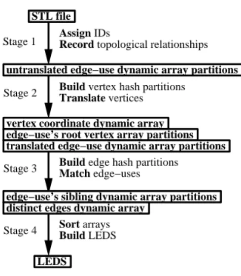
We make the only pass through the original input file during stage one. During this stage, we assign sequential edge-use and face IDs (recall that a LEDS face is really an oriented face-use) to each edge use and triangle in the input. We record the topo-logical relationships immediately available from the input, using a separate array for each type of relationship. These relationships are recorded using the IDs just assigned. We also record the vertex-use coordinates and other information we need to derive the remain-ing topological relationships. In stage two, we build a partitioned vertex hash table and use it to translate vertex-use coordinates to vertex IDs, and to derive the vertex topological relationships, creat-ing new arrays to hold them. In stage three, we build a partitioned edge hash table to match edge-uses with their siblings and record these relationships in additional arrays. In stage four, we fill in the actual LEDS elements. First we sort each array so that the entries appear in the same order as they will be recorded in the final LEDS. Then we read, in parallel, from the front of all the arrays containing vertex information to create the vertices. Next, the edge-uses and then faces are constructed by reading in parallel from their corre-sponding arrays. This allows us to write all of the information we need to record in each LEDS element at creation time, so that we do not need to go back and modify elements that have already been written out to disk.
Below, we describe these four stages in detail. Figure 5 shows a condensed summary of the four stages.
STL file Assign IDs
Record topological relationships
Stage 1
Stage 2 Build vertex hash partitionsTranslate vertices
untranslated edge−use dynamic array partitions
Stage 3
Stage 4
Build edge hash partitions Match edge−uses
Sort arrays Build LEDS LEDS
vertex coordinate dynamic array edge−use’s root vertex array partitions translated edge−use dynamic array partitions
edge−use’s sibling dynamic array partitions distinct edges dynamic array
Figure 5: The four main stages of the out-of-core algorithm. The
arrays of intermediate data created at each stage are shown in boxes.
7.1 Stage One
Recall that the two tasks in stage one are to assign IDs and record topological relationships in arrays. We use a separate counter for assigning sequential IDs to each type of LEDS element (vertex, edge-use, and face) so that we can also use the ID as an array in-dex for that element’s array. (Later, once we know the address for the start of each array, this allows us to translate IDs to pointers without any lookups using simple arithmetic.) For each triangle in the input, we can immediately assign new IDs for a face and its three edge-uses, since each is a unique use. We cannot immediately assign new vertex IDs, however. We do not know if each vertex is being encountered for the first time, in which case we need to assign it a new ID, or if it is a vertex that was already used in a tri-angle appearing earlier in the file, in which case we should use the ID already assigned to it. Therefore, in stage one, while we record
IDs for faces and edge-uses, we record the coordinate triples for the vertex-uses, waiting until we have built a vertex hash table in stage two to assign vertex IDs.
In the general case, we record data in five different dynamic ar-rays during stage one. Four of them record ID pairs, where the first ID is that of a LEDS element that will contain a pointer to a LEDS element with the second ID. These are the “edge-use’s face,” the “use’s next-in-loop use,” the “face’s outer loop edge-use,” and the “face’s inner loop edge-use” arrays. For triangulated input, none of the faces have inner loops; therefore, we clearly do not need this last array for STL. But for triangulated input we do not need to record these other three arrays either. The information they would contain can be derived later when we need it (as detailed in the description of stage four below) merely from knowing the total number of triangles and that the face and edge-use IDs are assigned as sequential integers.
The final array that we always create and fill during stage one will be used for deriving all of the remaining topological rela-tionships. It contains one entry per edge-use, but unlike in the four arrays described above, each entry is not a pair of IDs that translate directly to a pointer in the final LEDS. Instead an en-try contains three pieces of information: the ID of the edge-use, and the coordinates of the edge-use’s two endpoints’ vertex-uses. We call this the “untranslated edge-use” array because the vertex-use coordinates need to be translated to vertex IDs before we can interpret them as pointers. To prepare for the vertex translation in stage two, we output the untranslated edge-use array in parti-tions, appending each entry to the end of the appropriate partition:
ledsEdgeUseID = 1;
foreach triangle T in input {
v1Partition = GetPartition(T.v1Coords); UntranslatedEdgeUses[v1Partition].AppendTriple
(ledsEdgeUseID++,T.v1Coords,T.v2Coords); v2Partition = GetPartition(T.v2Coords); UntranslatedEdgeUses[v2Partition].AppendTriple
(ledsEdgeUseID++,T.v2Coords,T.v3Coords); v3Partition = GetPartition(T.v3Coords); UntranslatedEdgeUses[v3Partition].AppendTriple
(ledsEdgeUseID++,T.v3Coords,T.v1Coords); }
7.2 Stage Two
Stage two is the vertex hash table building and translation stage. If the input file is large, this hash table will not fit in memory; there-fore, we use a partitioned hash table. With partitioned hash tables, we only build one memory-sized piece (a “partition”) of a larger hash table at a time. Most Unix implementations now support the mlock()function, which we use to lock the partitions in memory while we are accessing them.
Using partitioned hash tables requires estimating how many hash table partitions we will need and dividing the input into that many data partitions before we process it. We take the hash value of the vertex, modulo the number of partitions, as the index of the data partition in which to store the input. This assures that all of the input corresponding to the same entry in the hash table will be in the same input data partition. Once the data is partitioned, we read one data partition at a time and build its corresponding hash table partition.
We translate the two endpoint vertices in the input in separate steps. For the first translation step, we partition the “untranslated edge-use” array based on the hash value of the edge-use’s first end-point’s coordinates. We try to predict the number of partitions that we will need from the size of the input file so that we can par-tition the “untranslated edge-use” array appropriately at creation time in stage one; the random hashing should make the partitions
of roughly equal size, so that the hash table for each will fit in mem-ory. If necessary we can re-partition the array when we build the hash tables.
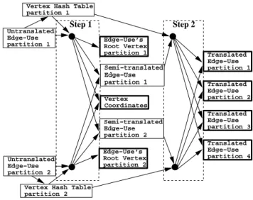
The input to stage two consists of the “untranslated edge-use” dynamic array partitions; the output consists of three new arrays: the “vertex coordinate” dynamic array, containing the vertex coor-dinates corresponding to each unique vertex ID, an “edge-use’s root vertex” array, containing each edge-use ID with the vertex ID for its corresponding root vertex, and a “translated edge-use” dynamic array with the same entries as the input untranslated edge-uses but with the vertex-use coordinates replaced by vertex IDs. Figure 6 shows the data flow between these arrays and the hash table parti-tions during both translation steps of stage two.
Untranslated Edge−Use partition 1 Untranslated Edge−Use partition 2
Vertex Hash Table partition 1
Vertex Hash Table partition 2 Step 1 Step 2 Semi−translated Edge−Use partition 2 Semi−translated Edge−Use partition 1
Stage Two
Vertex Coordinates Translated Edge−Use partition 1 Translated Edge−Use partition 2 Translated Edge−Use partition 4 Translated Edge−Use partition 3 Edge−Use’s Root Vertex partition 1 Edge−Use’s Root Vertex partition 2Figure 6: Data flow for the two vertex translation steps of stage
two. The output is indicated by bold boxes. We use the same hash table partitions for both steps but repartition and visit the hash table partitions in reverse order in step two. Note that there are more partitions at the end for the edge hash table we will build in stage three, since there are more edges than vertices.
Some of these arrays are static and some are dynamic. We out-put the “edge-use’s root vertex” information in one array per in-put partition, thus ensuring that each resulting array will also fit in memory (for later sorting). These arrays will have the same num-ber of entries as the input partitions; therefore, we can allocate them statically. On the other hand, the “translated edge-use” information needs to be partitioned differently than the input; therefore, we do not know its partition sizes and thus cannot allocate static arrays for them. We also do not know how many distinct vertices we will have; therefore, we must use a dynamic array to hold the vertex coordinates as well.
Before processing each “untranslated edge-use” partition, we al-locate its vertex hash table partition and lock it in memory. The input key to the vertex hash table is a coordinate triple, and the data stored in the hash table along with the key is the corresponding ver-tex ID.
After we have allocated the vertex hash table partition for the “untranslated edge-use” array partition, we perform the first ver-tex translation step (see Figure 7 for pseudo-code). We read each untranslated entry<Edge-Use ID, Endpoint 1 Coordinates, End-point 2 Coordinates>from the input partition in turn, and look up the coordinates of the middle field of the entry, Endpoint 1, in the vertex hash table partition. If the coordinates are not found in the hash table, we assign the next sequential vertex ID to these
co-ledsVertexID = 1;
foreach vertex-partition vP { allocate VtxHashTables[vP]; lock VtxHashTables[vP];
foreach triple <EdgeUseID,Vtx1Coords,Vtx2Coords> in UntranslatedEdgeUses[vP] {
VtxID = VtxHashTables[vP].LookUp(Vtx1Coords); if !(VtxID) { //it’s a new vertex
VtxID = ledsVertexID++;
VtxHashTables[vP].Insert(Vtx1Coords,VtxID); VtxCoordinates.Append(Vtx1Coords);
}
//output edge-use’s root vtx EdgeUseRootVertex[vP].AppendPair
(EdgeUseID,VtxID);
//repartition based on vtx2 hash value newP = GetPartition(Vtx2Coords); SemiTranslatedEdgeUses[newP].AppendTriple
(EdgeUseID,VtxID,Vtx2Coords); }
free UntranslatedEdgeUses[vP]; unlock VtxHashTables[vP]; }
Figure 7: Pseudo-code for stage two, vertex translation step one.
ordinates, record this vertex ID in the previously empty hash table entry, along with the coordinates, and append the coordinate triple as the ID-th entry in the “vertex coordinate” array. (When we pro-cess subsequent partitions, we use the same counter for assigning vertex IDs and output them to the same, unpartitioned, “vertex co-ordinate” array.) Otherwise, we read the previously assigned vertex ID from the hash table. This endpoint is the root vertex for the directed edge-use; we take its vertex ID along with the edge-use ID from the original entry and append the pair<Edge-Use ID, Vertex ID>to the current “edge-use’s root vertex” array partition. Finally, we replace the middle field of the original entry with the vertex ID and append the semi-translated triple,<Edge-Use ID, Vertex ID, Endpoint 2 Coordinates>, to the appropriate intermedi-ate “semi-translintermedi-ated edge-use” array partition. This time we choose the partition based on the hash value of the final field in the entry, the coordinates of Endpoint 2, since that is the next field we will be hashing. (The input was partitioned based on the hash value of the coordinates of Endpoint 1, which in general will be found in a different hash table partition than Endpoint 2; hence the need to re-partition.) Even though we are re-partitioning, however, we can still use static arrays, because each vertex appears the same number of times in both endpoint positions; therefore, the partitions will be the same size as last time. After processing each “untranslated edge-use” array partition, we free its memory. We unlock the cor-responding vertex hash table partition, allowing it to be paged out of memory, but do not free it yet.
In the second vertex translation step, we translate the second endpoint coordinate in each “semi-translated edge-use” to a ver-tex ID using the same hash table partitions we built in translation step number one (see pseudo-code in Figure 8). We process the partitions in the opposite order this time, starting with the “semi-translated edge-use” partition corresponding to the last vertex hash table partition that we built, since this hash table partition will still be in memory. Again, we lock each hash table partition in mem-ory while it is in use. We append the resulting translated triple,
<Edge-Use ID, Vertex ID, Vertex ID>, to the appropriate “trans-lated edge-use” array partition (this time basing the partition choice on the hash value of the edge, using the lexicographically ordered pair of vertex IDs as the hash key). We can free each vertex hash ta-ble partition and its corresponding “semi-translated edge-use” array partition after we finish processing it.
foreach vertex-partition vP { lock VtxHashTables[vP];
foreach triple <EdgeUseID,VtxID1,Vtx2Coords> in vSemiTranslatedEdgeUses[vP] {
VtxID2 = VtxHashTables[vP].LookUp(Vtx2Coords); // order endpoints lexicographically
if (VtxID1 < VtxID2) Key = (VtxID1,VtxID2); else
Key = (VtxID2,VtxID1); // Find edge-use partition
euP = GetPartition(Key);
TranslatedEdgeUses[euP].AppendTriple (EdgeUseID,VtxID1,VtxID2);
}
free VtxHashTables[vP];
free SemiTranslatedEdgeUses[vP]; }
Figure 8: Pseudo-code for stage two, vertex translation step two.
If the entire vertex hash table fits in memory and we are not par-titioning, then we can perform translation step two at the same time as step one, since we’ll always be looking at the same, lone hash table partition to find both vertex-use IDs for the triple. In fact, if we have not partitioned, then we could further optimize by look-ing up only one time each the three distinct vertex coordinates that appear as opposite endpoints of the three consecutive untranslated edge-use entries for a single triangle. This will halve the number of vertex-use lookups compared to the partitioned case. Further-more, the “edge-use’s root vertex” array for the unpartitioned case would not need to record the edge-use ID explicitly since they will be generated sequentially. Even if we have multiple partitions, some edges will still have both endpoints in the same partition. If we find upon hashing the second endpoint at the end of translation step one that it belongs in the same partition, we translate it im-mediately and output the fully translated triple directly instead of going through the semi-translated tables.
7.3 Stage Three
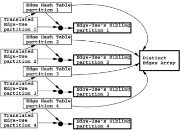
In stage three, we build a partitioned edge hash table in order to match up edge-uses that are on the same edge. We output an “edge-use’s sibling” dynamic array that records sibling pointer informa-tion, and also record the ID of one edge-use per edge in a “distinct edges” dynamic array (in stage four we will build the global linked list of edges for the LEDS from this array). Our input is the par-titioned “translated edge-use” array output in stage two, step two. Figure 9 shows the data flow during stage three.
Before processing each “translated edge-use” partition of
<Edge-Use ID, Vertex ID, Vertex ID>entries, we in turn allo-cate an edge hash table partition for it. Again, since we will be accessing the hash partition randomly, we lock it in memory. The input key to this hash table is the lexicographically ordered pair of vertex IDs of the endpoints of the edge-use (again, we use the lexi-cographic ordering to hide the direction of the original edge-use so that we can match it with the unoriented edge). When we output the partitioned “translated edge-use” array at the end of stage two, we based the partition choice on the hash value of this input key. In ad-dition to storing the input key, the edge hash table’s data field entry will store up to two use IDs for the edge, in the “first edge-use” field and the “most recent edge-edge-use” field (shown in Table 4), as detailed below and in pseudo-code in Figure 11.
Key Lesser Vertex ID Greater Vertex ID Data First Edge-Use ID Most Recent Edge-Use ID
Translated Edge−Use partition 1
Edge Hash Table partition 1
Translated Edge−Use partition 2
Edge Hash Table partition 2
Edge Hash Table partition 3
Edge Hash Table partition 4 Edge−Use’s Sibling partition 1 Edge−Use’s Sibling partition 2 Edge−Use’s Sibling partition 3 Edge−Use’s Sibling partition 4 Distinct Edges Array
Stage Three
Translated Edge−Use partition 3 Translated Edge−Use partition 4Figure 9: Data flow for stage three. The output is indicated by
bold boxes.
One partition of the “translated edge-use” array at a time, we look up each entry’s lexicographically ordered vertex IDs in the edge hash table partition we have allocated for it. If the edge is not found, we make a new entry for it in the hash table partition, recording the use ID (the first field of the “translated edge-use” input triple) in the “first edge-edge-use” field. We also append this edge-use ID to the “distinct edges” array.
If there is already an entry for the edge in the hash table partition, and it has the “first edge-use” data field filled but not the “most recent edge-use” field, this is the second edge-use for the edge. We read the data from the “first edge-use” field in order to append two new entries to the “edge-use’s sibling” array: one pair of edge-use IDs representing the pointer from the current to the first edge-use, and one pair of edge-use IDs representing the pointer from the first to the current use. Then we record the current triple’s edge-use ID in the “most recent edge-edge-use” field.
For input that was guaranteed to be 2-manifold, these first two edge-uses would be all the siblings for the edge; each edge-use of the pair would point to the other, its sole sibling. If this was the case for all edges, we would not need to record the most recent edge-use in the hash table. In fact, we could delete the edge’s whole entry after processing the second edge-use in order to free up more space in the hash table. But for non-manifold parts, we can have more than two edge-uses per edge.
When a non-manifold edge-use hashes to an edge entry that al-ready has both of its data fields filled by two other edge-uses for the edge, we also append two new entries to the “edge-use’s sibling” array (refer to Figure 10): one pair of edge-use IDs representing the pointer from the current triple’s edge-use to the “first edge-use” recorded in the hash table (as before), and one pair of edge-use IDs representing the pointer from the “most recent edge-use” recorded in the hash table to the current triple’s edge-use. This latter sib-ling pointer information will, when the actual LEDS edge-use is filled in, override the “edge-use’s sibling” pair we recorded when we processed the “most recent edge-use,” back when we recorded that its sibling was the first edge-use. In the LEDS, the sibling pointers of the edge-uses at each edge will thus form one circular list, though the order of the list will depend on the input file and will not necessarily be radially sorted. (We do radial sorting later and/or divide up the coincident edge-uses into pairs to make a pseudo-2-manifold representation if a particular application requires it.) Then we overwrite the “most recent edge-use” field in the hash table en-try with the current input enen-try’s edge-use ID, so that we can add additional siblings to the final circular list. Later, when we
pro-cess the “edge-use’s sibling” array, we will have two entries telling us what should be recorded in the sibling pointer field for some of these non-manifold edge-uses. We must be sure to take the latter one. edge−use’s sibling array additional entries: EU1EU2 EU2EU1 EU1EU3 EU3EU2 EU1EU4 EU4EU3 EU1 EU4 EU3 EU2 EU1 EU2 EU1 EU3 EU2 circular list thus far: hash table entry
(most recent EU overwritten): V1,V2 EU1 V1,V2 EU1EU2 V1,V2 EU1EU3 V1,V2 EU1EU4 V1 V2 key first EU most recent EU
non−manifold part non−manifold edge
EU4 EU3 EU2 EU1 V2 V1
Figure 10: We record each edge-use that hashes to an edge in one
of the data fields in the hash entry. If the “first edge-use” data field is full, we record it in the “most recent edge-use” data field and append two new entries to the “edge-use’s sibling” array, as illustrated. Interpreting each new sibling array entry to over-ride any previous entries for the same edge-use, we get the circular list shown on the right after each additional edge-use is added.
We repeat this process for each of the input partitions. We can free the memory for each “translated edge-use” array partition and its corresponding edge hash table partition after each has been pro-cessed, since they are not reused.
7.4 Stage Four
We wait until this final stage to actually allocate the LEDS vertices, edge-uses and faces. We fill in an array of one type of LEDS ele-ment at a time using the information in the intermediate arrays we have built, sorting them first (if not already sorted) by the ID of the LEDS element with which the relationship each entry describes will be stored. The larger input arrays will be stored in multiple parti-tions which individually fit in memory. We sort these partiparti-tions separately and then perform the final “merge” stage of a merge-sort implicitly: we keep a pointer to the next unprocessed entry in each partition of a partitioned array, and read from the partition we deter-mine contains the data for the next sequential ID being processed. We will only be making one sequential pass through each sorted partition during the merge; therefore, we will only need one block of each sorted partition in memory at a time.
foreach edge-use-partition euP { allocate EdgeHashTable[euP]; lock EdgeHashTable[euP];
foreach triple <EdgeUseID,VtxID1,VtxID2> in TranslatedEdgeUses[euP] { if (VtxID1 < VtxID2)
Key = (VtxID1,VtxID2); else
Key = (VtxID2,VtxID1);
Data = EdgeHashTable[euP].LookUp(Key); //first edge-use for edge
if (!Data) {
EdgeHashTable[euP].SetFirstEdgeUse (Key,EdgeUseID);
DistinctEdges.Append(EdgeUseID); }
//second edge-use for edge elseif (Data.FirstEdgeUse and
!Data.MostRecentEdgeUse) { EdgeUsesSibling[euP].AppendPair
(EdgeUseID,Data.FirstEdgeUse); EdgeUsesSibling[euP].AppendPair
(Data.FirstEdgeUse,EdgeUseID);
EdgeHashTable[euP].SetMostRecentEdgeUse (Key,EdgeUseID);
}
//subsequent edge-use for non-manifold edge elseif (Data.FirstEdgeUse and
Data.MostRecentEdgeUse) { EdgeUsesSibling[euP].AppendPair
(EdgeUseID,Data.FirstEdgeUse); EdgeUsesSibling[euP].AppendPair
(Data.MostRecentEdgeUse,EdgeUseID); EdgeHashTable[euP].SetMostRecentEdgeUse
(Key,EdgeUseID); }
}
free EdgeHashTable[euP]; free TranslatedEdgeUses[euP]; }
Figure 11: Pseudo-code for stage three.
We cannot fill in the edge-uses first because we will not have the information needed to fill in all of their fields until after we have processed the vertices. We do not fill in the faces first be-cause for triangulated input there is no intermediate face data that we can free after filling them in; therefore, we want to delay allo-cating the faces as long as possible to minimize the total memory requirements. Thus, we fill in the vertices first. Vertices point to edge-uses, and in order to derive these pointer values, we need to know the location of the final LEDS edge-use array; therefore, we must allocate it before filling in the vertices.
Now we allocate and prepare to fill in the data in the LEDS ver-tex array. We can fill in each LEDS verver-tex’s coordinates field di-rectly while reading sequentially from the “vertex coordinate” ar-ray, which is indexed by vertex ID; therefore, we do not need to do any additional preparation for that field. The information we need in order to fill in each vertex’s other field, the “first edge-use” field, is stored in the “edge-use’s root vertex” array partitions. Each of these partitions was created with the edge-use IDs in increasing (though not consecutive) order. Although we will need the infor-mation in that order later for the edge-uses, for the vertices we sort each of these partitions by vertex ID to put them in the order in which we will create the vertices and to bring all of the edge-uses for a single vertex together. (We could make a separate copy to sort in vertex ID order, but it is actually more efficient to sort and
f(n)=3n f(n)= (n)mod3 n+1
{
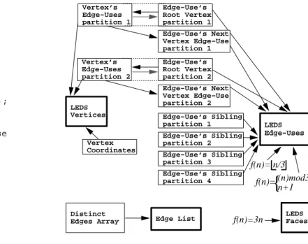
f(n)= n/3 Edge−Use’s Sibling partition 1 Edge−Use’s Sibling partition 2 Edge−Use’s Sibling partition 3 Edge−Use’s Sibling partition 4 Vertex Coordinates Edge−Use’s Root Vertex partition 2 Vertex’s Edge−Uses partition 2 Edge−Use’s Next Vertex Edge−Use partition 2 LEDS Edge−Uses LEDS Vertices LEDS Faces DistinctEdges Array Edge List
Edge−Use’s Root Vertex partition 1 Vertex’s Edge−Uses partition 1 Edge−Use’s Next Vertex Edge−Use partition 1
Figure 12: Data flow for stage four. The output is indicated by
bold boxes. The input consists of the “edge-use’s sibling” parti-tions output in stage three, as well as the vertex coordinates and “edge-use’s root vertex” partitions output in stage two, step one.
then re-sort back to the original order.) Since the “edge-use’s root vertex” array partition was built from a single hash partition, parti-tioned based on vertex coordinates, all of the edge-uses for a single vertex will appear in the same partition. Thus we can maintain the same partitions (which will again fit in memory) and sort within each to get a “vertex’s edge-uses” ordered array.
7.4.1 LEDS Vertices
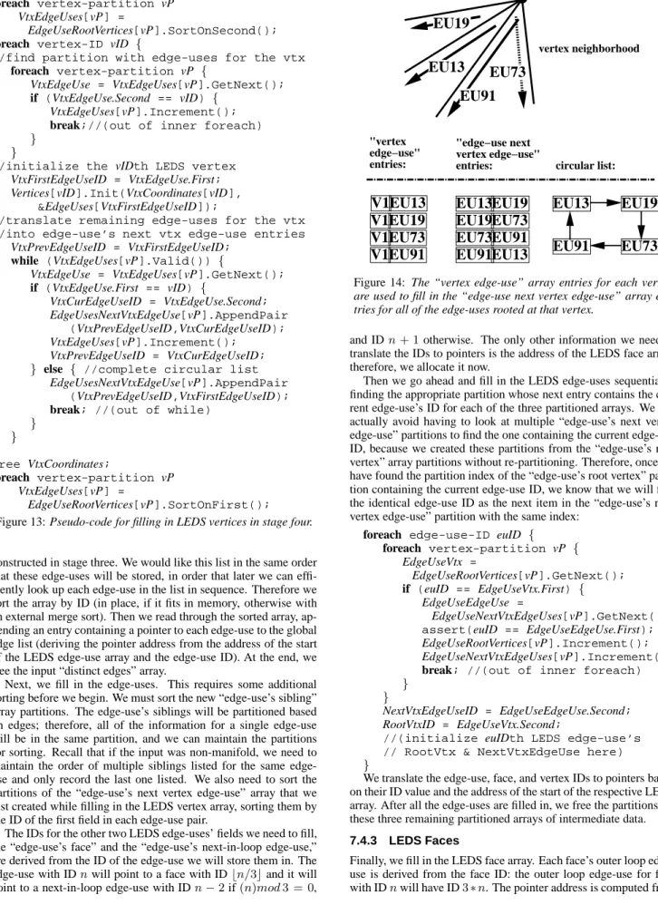
Now we have all the data ready in the correct order to fill in the vertices sequentially. (Pseudo-code for these operations is given in Figure 13.) We find the coordinates of the current vertex immedi-ately from the next entry in the “vertex coordinate” array. For the vertex’s first edge-use, we find the “vertex’s edge-uses” partition whose next entry contains the current vertex’s ID. There will be several entries for this vertex, corresponding to all of its edge-uses. We record its first edge-use entry in the LEDS vertex, translating the edge-use to a pointer based on its ID and the address of the LEDS edge-use array. The vertex’s remaining edge-uses will be stored in the edge-uses themselves.
Now that we have grouped the edge-uses together by root ver-tex, we can output entries for the “edge-use’s next vertex edge-use” array (refer to Figure 14). We read each additional sequential entry for the current vertex from its “vertex’s edge-uses” input partition and append a pair of edge-use IDs to the corresponding partition of the “edge-use’s next vertex edge-use” array: the ID of the prior edge-use for the current vertex just read from the input, and the ID of the edge-use in the current entry. After processing the last en-try for the current vertex, we also output a pair of IDs to link its edge-use back to the first edge-use for the vertex. These pairs will be translated to the pointers in the LEDS edge-uses that will form a circularly linked list of all the edge-uses rooted at the vertex.
After we have filled in all of the LEDS vertices, we can free the vertex coordinate array. We do not free the “vertex’s edge-uses” partitions, but instead re-sort each by edge-use ID (back to its orig-inal “edge-use’s root vertex” order).
7.4.2 LEDS Edge-Uses
Along with the LEDS edge-uses, we build the global linked list of pointers to one edge-use per edge from the “distinct edges” array
//sort edge-uses by root vertex foreach vertex-partition vP
VtxEdgeUses[vP] =
EdgeUseRootVertices[vP].SortOnSecond(); foreach vertex-ID vID {
//find partition with edge-uses for the vtx foreach vertex-partition vP {
VtxEdgeUse = VtxEdgeUses[vP].GetNext(); if (VtxEdgeUse.Second == vID) {
VtxEdgeUses[vP].Increment(); break;//(out of inner foreach) }
}
//initialize the vIDth LEDS vertex
VtxFirstEdgeUseID = VtxEdgeUse.First; Vertices[vID].Init(VtxCoordinates[vID],
&EdgeUses[VtxFirstEdgeUseID]);
//translate remaining edge-uses for the vtx //into edge-use’s next vtx edge-use entries
VtxPrevEdgeUseID = VtxFirstEdgeUseID; while (VtxEdgeUses[vP].Valid()) {
VtxEdgeUse = VtxEdgeUses[vP].GetNext(); if (VtxEdgeUse.First == vID) { VtxCurEdgeUseID = VtxEdgeUse.Second; EdgeUsesNextVtxEdgeUse[vP].AppendPair (VtxPrevEdgeUseID,VtxCurEdgeUseID); VtxEdgeUses[vP].Increment(); VtxPrevEdgeUseID = VtxCurEdgeUseID;
} else { //complete circular list
EdgeUsesNextVtxEdgeUse[vP].AppendPair (VtxPrevEdgeUseID,VtxFirstEdgeUseID); break; //(out of while)
} } } free VtxCoordinates; foreach vertex-partition vP VtxEdgeUses[vP] = EdgeUseRootVertices[vP].SortOnFirst(); Figure 13: Pseudo-code for filling in LEDS vertices in stage four.
constructed in stage three. We would like this list in the same order that these edge-uses will be stored, in order that later we can effi-ciently look up each edge-use in the list in sequence. Therefore we sort the array by ID (in place, if it fits in memory, otherwise with an external merge sort). Then we read through the sorted array, ap-pending an entry containing a pointer to each edge-use to the global edge list (deriving the pointer address from the address of the start of the LEDS edge-use array and the edge-use ID). At the end, we free the input “distinct edges” array.
Next, we fill in the edge-uses. This requires some additional sorting before we begin. We must sort the new “edge-use’s sibling” array partitions. The edge-use’s siblings will be partitioned based on edges; therefore, all of the information for a single edge-use will be in the same partition, and we can maintain the partitions for sorting. Recall that if the input was non-manifold, we need to maintain the order of multiple siblings listed for the same edge-use and only record the last one listed. We also need to sort the partitions of the “edge-use’s next vertex edge-use” array that we just created while filling in the LEDS vertex array, sorting them by the ID of the first field in each edge-use pair.
The IDs for the other two LEDS edge-uses’ fields we need to fill, the “edge-use’s face” and the “edge-use’s next-in-loop edge-use,” are derived from the ID of the edge-use we will store them in. The edge-use with IDnwill point to a face with IDbn/3cand it will point to a next-in-loop edge-use with IDn−2if(n)mod3 = 0,
"vertex edge−use" entries:
V1EU13
V1EU19
V1EU73
V1EU91
EU13EU19
EU19EU73
EU73EU91
EU91EU13
"edge−use next vertex edge−use" entries:V1
EU91
EU13
EU73
EU19
circular list:EU13
EU19
EU73
EU91
vertex neighborhoodFigure 14: The “vertex edge-use” array entries for each vertex
are used to fill in the “edge-use next vertex edge-use” array en-tries for all of the edge-uses rooted at that vertex.
and IDn+ 1otherwise. The only other information we need to translate the IDs to pointers is the address of the LEDS face array; therefore, we allocate it now.
Then we go ahead and fill in the LEDS edge-uses sequentially, finding the appropriate partition whose next entry contains the cur-rent edge-use’s ID for each of the three partitioned arrays. We can actually avoid having to look at multiple “edge-use’s next vertex edge-use” partitions to find the one containing the current edge-use ID, because we created these partitions from the “edge-use’s root vertex” array partitions without re-partitioning. Therefore, once we have found the partition index of the “edge-use’s root vertex” parti-tion containing the current edge-use ID, we know that we will find the identical edge-use ID as the next item in the “edge-use’s next vertex edge-use” partition with the same index:
foreach edge-use-ID euID { foreach vertex-partition vP { EdgeUseVtx = EdgeUseRootVertices[vP].GetNext(); if (euID == EdgeUseVtx.First) { EdgeUseEdgeUse = EdgeUseNextVtxEdgeUses[vP].GetNext(); assert(euID == EdgeUseEdgeUse.First); EdgeUseRootVertices[vP].Increment(); EdgeUseNextVtxEdgeUses[vP].Increment(); break; //(out of inner foreach) }
}
NextVtxEdgeUseID = EdgeUseEdgeUse.Second; RootVtxID = EdgeUseVtx.Second;
//(initialize euIDth LEDS edge-use’s
// RootVtx & NextVtxEdgeUse here) }
We translate the edge-use, face, and vertex IDs to pointers based on their ID value and the address of the start of the respective LEDS array. After all the edge-uses are filled in, we free the partitions for these three remaining partitioned arrays of intermediate data.
7.4.3 LEDS Faces
Finally, we fill in the LEDS face array. Each face’s outer loop edge-use is derived from the face ID: the outer loop edge-edge-use for face with IDnwill have ID3∗n. The pointer address is computed from
the address of the edge-use array and the edge-use ID. The inner loop list pointer for each face is null for triangulated input.
8
Results
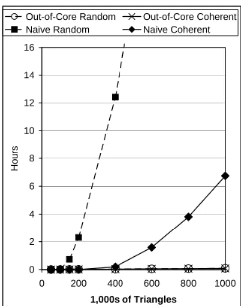
For comparison with the naive in-memory algorithm, we ran the out-of-core algorithm on the same knot sculpture files, again under Linux with 32 MB of RAM. For smaller files, where all or most all data fits in memory, the out-of-core algorithm can take up to three times longer to build the LEDS than the naive algorithm, due to the time required to write the intermediate data. For our coher-ent input files, the break-even point comes after 400,000 triangles; for random input, break-even comes after 70,000 triangles (see Fig-ure 15). With the million triangle test part, we more than make up for the overhead of the intermediate data with drastically reduced thrashing. For the coherent million triangle test part, the naive algo-rithm takes 82 times as long as the out-of-core algoalgo-rithm. For the randomized million triangle test part, the naive algorithm was so slow that we had to terminate it after two days, but the out-of-core algorithm performs almost identically on the coherent and on the randomized million triangle inputs, at just under and just over five minutes, respectively. For the largest randomized file on which we successfully ran the naive algorithm, the 600,000 triangle test part, the naive algorithm took over 500 times as long as the out-of-core algorithm. 0 2 4 6 8 10 12 14 16 0 200 400 600 800 1000 1,000s of Triangles H o u rs
Out-of-Core Random Out-of-Core Coherent Naive Random Naive Coherent
Figure 15: Comparison of in-memory and out-of-core algorithm
LEDS build times on large knot sculpture files under Linux with 32 MB RAM. The out-of-core algorithm performs equally well on the coherent and non-coherent input. The naive algorithm takes 82 times as long as the out-of-core algorithm on the coherent mil-lion triangle input, and over 500 times as long on the randomized 600,000 triangle input.
Typical parts are neither quite as coherent as the original knot sculpture test files nor as random as the randomized versions. For other parts of a similar size, we would expect speed-ups somewhere in between 82 and 500 times. To test this hypothesis, we ran the naive and out-of-core algorithms on an STL file of the Stanford dragon reconstructed from laser range finder data which contained 870,000 triangles, again using 32 MB of RAM. On average it took 9 hours and 15 minutes with the naive algorithm, but only 4 min-utes and 11 seconds with the out-of-core algorithm, a speed-up of a factor of 133.
9
Memory Usage
If the out-of-core algorithm is not implemented carefully, it can re-quire far more virtual memory than the in-memory algorithm, in order to store its intermediate data. To minimize its virtual mem-ory requirements, we free each intermediate array and hash table partition as soon as we have finished processing it, so that we can re-use the memory. With this careful memory management, our out-of-core implementation uses almost exactly the same amount of memory as the memory algorithm (see Figure 16). For the in-memory algorithm, both hash tables are built simultaneously, and we cannot free them until the entire LEDS is built. For the out-of-core algorithm, we build the hash table partitions sequentially, freeing the vertex hash table before allocating the edge hash table, and freeing them both before allocating the LEDS. We also allocate the LEDS vertices, edge-uses, and faces in stages, allowing us to free all of the remaining intermediate data before finally allocating the LEDS faces. An additional advantage of the out-of-core algo-rithm is that most of the intermediate and all of the final arrays can be allocated in the exact size needed, so that less memory is wasted.
0 100 200 300 400 200, 000 400, 000 600, 000 800, 000 1,00 0,00 0 Number of Triangles M B y te s
Out-of-core algorithm In-memory algorithm
Figure 16: Comparison of memory usage for the out-of-core and
in-memory algorithms on different sized knot sculpture files.
10
Spatial Partitioning
The general out-of-core algorithm described, while it builds a topo-logical data structure very efficiently, may not be optimal when con-sidered together with the running time of the application that uses the LEDS. This is because it may not organize the data within the LEDS optimally, depending on the access patterns of the particular application that will be using the data. An application can always re-sort the arrays of vertices, edge-uses, and faces after they have been constructed, but if we already know what application will be using the data structure, we might be able to build it so that its order is better tuned to the access patterns of that application in the first place. Often, a spatially coherent organization is desirable.
With the basic build algorithm, faces and edge-uses are stored in the same order that they appear in the input. If there is spatial coher-ence in the input, it will be preserved in the LEDS. For triangulated input, we exploit the simple numeric relationships between the face IDs and edge-use IDs to avoid having to record this information in intermediate arrays. Thus any advantages from changing the IDs at the start to induce a different ordering, rather than re-sorting at the end, would be offset by the added overhead of these new interme-diate arrays. Therefore, there would be little advantage to changing
the order of the faces and edge-uses during the initial build, unless the input was known to be non-coherent.
The basic build algorithm can destroy any input coherence in the case of the vertices, however. The vertex uses are randomly assigned to partitions during the initial read of the data; if there are many partitions, this will effectively shuffle them when the vertex IDs are assigned sequentially within each partition. Therefore, it might be worthwhile to wait until after the first pass through the data to partition for vertex hashing. This would allow us to gather statistics on the distribution of the vertices during the initial read, so that we could divide the vertex-uses into partitions that were spatially coherent and still had roughly equal sizes.
When we process a file for solid freeform fabrication, we must slice it into closely spaced parallel layers. We perform these slice calculations using a sweep-plane slicer that looks at the vertices in increasing z-coordinate order [17]. Therefore, we have imple-mented a spatial partitioning scheme that divides the vertices into partitions based on increasingz-coordinate.
We do not know thez-extents or distribution of the data before we begin, which prevents us from knowing where to place the par-tition boundaries for equal parpar-tition sizes a priori. During the first pass through the triangle input data, we merely record a single dy-namic array of the vertex coordinates of each sequential input tri-angle, and find the minimum and maximumz value for the file. We still do not know the distribution inz; therefore we first evenly divide the range of inputzvalues into small intervals, many more than the final number of partitions we need, and later combine con-secutive intervals into partitions of even sizes. (Our intervals are not unlike the buckets used by Kitsuregawa et al. to tune partition sizes during hash joins [13], but we simultaneously sort and tune with our intervals, optimizing for processing that will occur after the ini-tial spaini-tial hash join as well.) We allocate a bin for each sequen-tial interval, with the first bin corresponding to the lowest interval. Then we read through the array of vertex coordinates, transforming each set of three vertices defining a triangle into three “untranslated edge-use” entries, storing each entry in the bin corresponding to the interval containing thez-coordinate of its first endpoint. We also update an array that records the number of entries that have been placed in each bin.
Then we look at the bin sizes and contents to assign partition boundaries to get partitions of roughly equal sizes. The ideal parti-tion size is equal to the total number of entries divided by the total number of partitions. For the first partition, we add up the number of entries in the firstibins until the total first reaches a number greater or equal to the ideal partition size. If the total is less than or equal to 10% over the ideal size, bins 1 toiwill be the parti-tion. Otherwise, we subtract the number of entries in theith
bin, and if this total is greater than or equal to 10% under the ideal size, bins 1 toi−1will be the partition. In either case, thez-boundary of the partition is calculated and recorded (the highest bin number times the constant binz-height for the first partition). Otherwise, we will have to divide theith
bin between the first and second par-titions (this will only occur if we allocated too few bins or if the vertex data is very unevenly distributed inz). Our implementation performs a quicksort on the whole bin and then finds the entry at the position for an ideal partition size; we record thezcoordinate of this edge-use’s first endpoint as thez-boundary of the partition. For better performance, we could modify the quicksort to terminate once we had an acceptable number of entries less than the pivot point and use the pivot point for thez-boundary. Since we rarely need to split bins, the additional complexity of modifying quicksort did not seem worthwhile.
We continue in this manner to find thez-boundaries of the re-maining partitions, but rather than trying to get the size of each individual partition within 10% of the ideal size, we aim for the sum of the sizes of the partitions so far plus the current one to be
within 10% of the sum of the ideal sizes. This prevents errors from building up, which could leave the final partition, consisting of all remaining entries, constrained to be much too small or too large. With our scheme, individual partition sizes will, in the worst case, still be no more than 20% larger or smaller than the ideal size.
Recall that we partition vertices twice: once to translate the first endpoint in the untranslated edge-uses, then again to translate the second endpoint in the semi-translated edge-uses. For the first par-titioning step, we build our hash tables and translate directly from the bins that thez-boundary table indicates belong entirely to the current partition (along with possibly a fraction of the end bin(s), if they were split). When we repartition the output of this first transla-tion step, we actually allocate partitransla-tions, using thez-boundary table to place the output in the correct partition. The rest of the build pro-ceeds as before.
The bins, in addition to aiding in partitioning evenly, also roughly sort the vertices within the partitions. During the first trans-lation step, we process the bins in order; recall that it is also in the first translation step that we assign IDs to the vertices in the order that we process them. Therefore, the final vertex table will be sorted to the same granularity as the bin boundaries. More bins will result in a finer sort.
Of course, the bin partitioning scheme takes longer than random partitioning. In Figure 17, we compare the total times to build the LEDS followed by slicing with the sweep plane slicer under Linux with 32 MB RAM. Our input is the 200,000 triangle knot sculpture,
0 20 40 60 80 100 120 Random Partitioning 250 bins 1000 bins S e c o n d s
LEDS build time Slice time
Figure 17: Comparison of build times versus slice times for
ran-dom partitioning andz-coordinate based vertex partitioning with different bin sizes, using the 200,000 triangle knot sculpture as input.
we make a total of 402 slices through it, and we use 10 partitions. Allocating 250 bins total (25 bins per partition on average), the total build plus slice time was faster than with random partitioning, even though the build time was longer. Using 1,000 bins (100 bins per partition), the build time increased even more, and the savings in analyzing and slicing no longer offset the increased build time.
11
Conclusion
We have described the design and implementation of an out-of-core algorithm for building a topological data structure from unorga-nized input. We have demonstrated performance improvements of two orders of magnitude over a naive approach by using our new al-gorithm. Unlike some algorithms that trade off space for speed, we are able to achieve these speed-ups without increasing the virtual