Take it or Leave it: Take-up, Optimal Transfer Programs, and Monitoring

Take it or Leave it: Take-up, Optimal Transfer

Programs, and Monitoring

Laurence Jacquet

CES

IFO

W

ORKING

P

APER

N

O

.

3018

CATEGORY 1: PUBLIC FINANCE

APRIL 2010

An electronic version of the paper may be downloaded

• from the SSRN website: www.SSRN.com

• from the RePEc website: www.RePEc.org

CESifo Working Paper No. 3018

Take it or Leave it: Take-up, Optimal Transfer

Programs, and Monitoring

Abstract

This paper studies the optimal income redistribution and optimal monitoring when disability

benefits are intended for disabled people but when some able agents with high distaste for

work mimic them (type II errors). Labor supply responses are at the extensive margin and

endogenous take-up costs may burden disabled recipients (because of either a reputational

externality caused by cheaters or a snowball effect). Under paternalistic utilitarian preferences

that do not compensate for distaste for work, inactive disabled recipients should obtain strictly

lower consumption than disabled workers. The cost of monitoring supports adoption of an

Earned Income Tax Credit. However, and surprisingly, with or without take-up costs, even if

perfect monitoring is costless, it proves optimal to have type II errors. These results are robust

to a utilitarian criterion. The paper provides numerical simulations calibrated on U.S. data.

JEL-Code: H21.

Keywords: optimal income taxation, tagging, take-up, extensive margin.

Laurence Jacquet

Norwegian School of Economics and Business Administration

Helleveien 30

5045 Bergen

Norway

laurence.jacquet@nhh.no

March 1, 2010

In particular, I am extremely grateful to Katherine Cuff. She was particularly helpful in

providing suggestions and comments at various stages of the analysis. I would also like to

thank Philippe De Donder, Gregory Corcos, Gernot Doppelhofer, Timothy J. Goodspeed,

Eirik Kristiansen, Laurent Simula, Erwin Ooghe, Stéphane Robin, Agnar Sandmo, Dirk

Schindler, Fred Schroyen, Dirk Van de gaer and several participants at the 2009 CESifo

Conference on Public Sector Economics for their advice on a previous version. The scientific

responsibility is assumed by the author.

1

Introduction

This paper examines the optimal redistributive structure and the optimal accuracy of monitoring when disability bene…ts are intended for disabled people but where some able agents who have a high distaste for work mimic them. It suggests the shape of the optimal tax-transfer system when the government operates a costly monitoring program …nanced by taxation of labor income.

The standard optimal taxation model assumes that individuals are distributed over some private characteristic, such as their individual productivity, the distribution of which is common knowledge. Redistribution policy is limited by incentive constraints that must be satis…ed if individuals are to reveal their true productivity types (Mirrlees, 1971). These incentive compatibility constraints are relaxed and redistribution is enhanced when some characteristics correlated with low productivity (or ‘tag’to use the terminology introduced by Akerlof, 1978), like disability status, are monitored for a subset of the disabled population.1

This paper di¤ers from the existing literature by endogenizing the monitoring technology2 and all of the behavioral responses (participation to the labor market and to disability programs), which allows us to cast light on three important redistributive issues.

First, who gets the largest consumption level? The tagging literature shows that tagged disabled agents obtain a larger consumption level than untagged disabled people (e.g., Akerlof, 1978; Salanié, 2002). This result relies on the assumption that eligible people do not work whether they are tagged or untagged. However, some disabled people work, and others do not work and receive disability bene…ts in the real world.3 _{This paper models behavioral responses such as labor supply responses}

and take-up responses as accurately as possible and shows that the optimal ranking of consumption bundles is then reversed to give work incentives to some disabled.

Secondly, who gets the largest transfer? By de…nition, an Earned Income Tax Credit (EITC) provides the largest transfer to disabled or low-productivity workers. This contrasts with a Negative Income Tax (NIT), whereby nonemployed agents receive the largest transfer. As usual in the literature, let us de…ne the ratio of social marginal utility to the marginal value of public funds as the marginal social welfare weight. Neglecting monitoring, the literature has well established that when labor supply responses are modeled along the extensive margin (i.e., the agent decides whether or not to participate in the labor force), a marginal social welfare weight lower (larger) than one on disabled workers implies a NIT (EITC) (Diamond, 1980; Saez, 2002). Contrastingly, this paper shows that, with a costly monitoring technology, a marginal social welfare weight lower than one on disabled workers does not preclude an EITC.

Third, relaxing the standard assumption that monitoring, and therefore the probability of

1_{In this paper, the tag (disability) is perfectly correlated with low productivity, which is the basis for}

redistri-bution. However, the tag is not perfectly observable; hence, tagging is not perfect. Contrastingly, in the seminal paper of Akerlof (1978), the tag is perfectly observable but correlated more or less perfectly with low productivity. Tagging is also not perfect.

2_{An exception is Boadwayet al. (1999), where the accuracy of monitoring depends on the e¤ort level of social}

workers. Boadway et al. (1999) characterize the optimal payment and monitoring of social workers who shirk. Shirking induces errors in screening between disabled and low-ability claimants (the latter are the able in our model). Contrastingly, the endogenous monitoring of our model depends upon the resources devoted to it and there is no agency problem involved in the tagging process. We also relax Boadway etal.’s assumption that government policy is designed such that all low-ability and disabled people apply for welfare assistance. The other di¤erences between our model and that of Boadwayet al. (1999) will become apparent as we proceed.

3_{In EU countries, about 30% of people who report severe disability do not get disability bene…ts and work}

errors, is taken as given, this paper shows that there should always remain some type II errors (i.e., able people who falsely claim to be disabled and receive disability bene…ts). When the marginal cost of monitoring is very high, no monitoring (hence a type II error probability of one) is optimal. More surprising, even when monitoring is perfect and costless, it is optimal that some type II errors prevail. Since labor supply is restricted to be binary, the direct truthful mechanism that implements the optimal allocation is never fully revealing. Therefore, to reach the ideal full information allocation, the tax authority needs to not only observe the correct health status of claimants by its monitoring, but must also observe their precise disutility if they worked. Since perfect monitoring provides correct information on the health status of claimants but not on their disutility from work, having some people who commit fraud is optimal, under asymmetric information.

In this paper, optimal tax formulas are derived to provide a clear understanding of the key economic e¤ects underlying them. This allows better analysis of the new e¤ects that monitoring and take-up imply for standard formulas. To ease the comparison with the existing literature, these formulas are presented as functions of the behavioral elasticities.

Non-take-up may exist because of the costs of learning about and applying for the program or because of stigma costs (e.g., Sen, 1995; Currie, 2006). This paper emphasizes the endogenous stigma à la Besley and Coate (1992) as an explanation of the non-take-up phenomenon. Given the imperfect observability of disability,4 _{there are recipients whose decision to claim bene…ts can be}

directly attributed to laziness and not to disability. When one is truly disabled, being considered as an undeserving (i.e., lazy) recipient is demeaning and stigmatizing. This stigma increases with the number of cheaters. Although no empirical papers have studied this endogenous stigma, anecdotal evidence about people who cheat in welfare programs and then create doubts or social resentment against their peers seems persistent enough to open the path to more investigation. To the best of our knowledge, the endogenous stigma à la Besley and Coate has never been studied in the optimal income tax and tagging literature. Our optimal tax formula then includes all e¤ects that arise from the stigma externality. Moreover, this paper also studies the robustness of the optimal tax formula to an alternative take-up cost function. Importantly, all of our results are also valid without any take-up cost.

The analysis is realized under a normative criterion corrected for features that individuals are responsible for (Bossertet al., 1999; Schokkaert et al., 2004). According to this paternalistic ap-proach, income should not be transferred as compensation for distaste for work because individuals are responsible for their own taste for work. Moreover, disabled workers, contrary to the lazy ones, ought to be compensated for their handicap. The validity of our main results is examined and con…rmed under a utilitarian criterion.

We proceed in the following section by setting up the basic model. Assuming the paternalistic criterion, Sections 3 and 4 derive the optimal tax-transfer and monitoring programs under full information and asymmetric information, respectively. Section 5 studies the robustness of the results under a utilitarian criterion. Section 6 presents some numerical results.

4_{In 2005, about 80% of disability recipients su¤er from mental disorders and musculoskeletal diseases (e.g.,}

back pain) (Social Security Administration, 2006). Generally, most of these disabilities are neither easily observed nor perfectly monitored, even with a deep medical examination (Campioleti, 2002). Therefore, disability transfer systems are always imperfect. Benitez-Silvaet al. (2004b) estimate that approximately20%of applicants who are ultimately awarded bene…ts are not disabled.

2

The model

2.1

Individual’s behavior

Agents are either able or disabled. Productivities take two values,wH > wL>0, which correspond

with the gross wages in two types of jobs (low and high skilled). Nd is the proportion of disabled

people in the population. Their productivity is wL. Na 1 Nd is the proportion of able people

in the population whose productivity iswH. There is a perfect correlation between disability and

lower productivity. This assumption is in the vein of the statutory de…nition of disabled people who are eligible for disability bene…ts. The applicant is considered to be disabled not just because of the existence of a medical impairment, but because the impairment drastically reduces his or her productivity and precludes any substantial and gainful work (Hu et al., 2001). A disabled worker in a wheelchair who has the functional capability to engage in a substantial gainful job is not considered disabled either by the U.S. Social Security Act or in this model.

Assume that agents decide whether or not to work. This assumption seems natural since the empirical literature has shown that the extensive margin of labor responses is important, especially at the low income end (e.g., Meghir and Phillips, 2008) while most estimates of hours of work elasticities conditional on working are small (Blundell and MaCurdy, 1999). Utility is quasilinear and represented by:

v(x) if they work,

v(x) Iif they do not work,

where xis consumption, v(x) :R+ _{! R:x!v(x)with v}0 _{>0 v}00 _{and limx}

!1v0(x) = 0,

is a parameter measuring disutility when working,Iis an indicator function that takes the value of1if inactive agents take-up disability bene…ts and0 otherwise, and denotes the (endogenous) take-up cost.

The disutility of work is denoted d for the wL-agents and a for the wH-agents. d is

distributed according to the cumulative distribution functionF( d) :R+![0;1] : d!F( d)and

the corresponding density functionf( d). The latter is continuous and positive over its domain. a

is distributed according to the cumulative distribution functionG( a) :R+ ![0;1] : a !G( a)

and the corresponding (continuous and positive) density functiong( a).5 Individual characteristics

are private information to each person while the distribution thereof is assumed to be public information.

The rest of this section de…nes the endogenous take-up cost in the utility function. Let us already emphasize that all results of this paper are still valid when those take-up costs are neglected, i.e., = 0, which is the standard assumption in the optimal taxation and tagging literature.

Stigma and snowball take-up costs

We now de…ne the take-up cost (:)that can be stigma or the take-up cost of snowball. The phenomenon that disabled recipients are viewed with some suspicion and are vulnerable to accusations of laziness has largely been documented by psychologists and sociologists since Go¤man

5_{We want to see whether an EITC or a NIT is optimal. This requires us to describe only the participation tax}

rates. Therefore, it is appropriate to assume a discrete support for skills, like in Saez (2002). For simplicity, we assume two productivity levels, but increasing the number of productivities would not modify our main results. Continuity of is assumed for simplicity.

(1963). However, to the best of our knowledge, the economics literature has largely neglected that being considered as an undeserving (i.e., lazy) recipient when one truly is disabled is demeaning and stigmatizing. This motivates our focus on the reputational stigma à la Besley and Coate (1992). The undeserving (able) recipients impose a “reputational externality” (Besley and Coate, 1992) on the deserving (disabled) ones.6 When it is known that an individual is receiving disability bene…ts, other individuals infer that this individual is probably lazy.7 This creates the reputational stigma that reduces the recipients’ utility. Stigma is an increasing function of the proportion of undeserving recipients in the economy, denoted by u

a. The undeserving bene…ciaries are able

agents who do not work, i.e., they are “voluntarily unemployed”; hence, the subscriptsaanduare used. It seems realistic to assume that reputational stigma hurts deserving people more than the undeserving because the former face a limited choice set. The cost of being perceived as a cheater is lower for someone who does commit fraud (i.e., an able recipient) than for someone who does not (i.e., a disabled recipient). Without a¤ecting the qualitative nature of the results but to later ease the notations and intuitions, we assume zero stigma e¤ect for the able recipients. However, our results are still valid when able people also face positive stigma and the optimal tax formulas could easily be written with larger stigma on the cheaters than on the deserving.8

The de…nition of stigma of Besley and Coate (1992) is relevant if we consider a society where people who do their best abiding by the rules are respected and admired (even if they are quasi-unproductive) and where people who do not comply with the rules (even in a cunning way) are despised. If we want to model a society where cheats and “old foxes” are admired, stigma should be a decreasing function of u

a. The take-up by undeserving people then has a snowball e¤ect on

take-up by the deserving.9

The type of take-up cost then depends on the …rst derivative: Stigma (snowball take-up cost) prevails when 0( u_a)>0 ( 0( u_a)< 0). The rest of the paper will mainly focus on the general form 0₍ u

a), letting the reader choose the type of take-up cost she/he prefers.

2.2

The government’s decisions

A feature of disability systems is that the eligibility of applicants is assessed on the basis of the disability status rather than being solely dependent on reported incomes. The process of

6_{Society is deemed to value certain individual characteristics, such as willingness to earn one’s income from}

work when one is able to do so (e.g., Sen, 1995; Lindbeck et al., 1999). A social norm claiming that disabled, low-productivity people should get transfers also prevails (e.g., Wol¤, 2004). Given the imperfect observability of disability, there are (lazy) able agents who do not deserve bene…ts but receive them.

7_{Anecdotal evidence about this reputational stigma e¤ect also exists in politics or sport. For instance, during}

the 2006 Tour de France, when several exceptional cyclists were revealed to have taken drugs to improve their performances, the entire profession lost its credibility and all cyclists were suspected of being cheats.

8_{Introducing larger stigma on the able applicants than on the disabled ones implies that take-up costs are an}

ordeal associated with desirable screening (e.g., Nichols and Zeckhauser (1982) and Cu¤ (2000)).

9_{Rather than explaining the snowball e¤ect with a society where cheats and old foxes are admired, alternative}

empirical explanations can prevail. In the vein of recent empirical studies that look at endogenous social interactions and peer e¤ects (e.g., Aizer and Currie, 2004), it can become less embarrassing to live on transfers when more individuals do likewise (Lindbecket al., 1999). Alternatively, the snowball e¤ect can be explained by complexity or the rigor of the monitoring technology, see Kleven and Kopczuk (2010) for a model of transfer program complexity (however, without tax revenue and without administrative costs). Complexity is an instrument used by program administrators to increase the intensity of screening, hence to reduce errors. Higher complexity requires larger governmental expenditure per applicant, e.g., because of the increased number of tests and interviews with doctors. Larger monitoring expenditure per applicant reduces u

a, as it will be made explicit in Section 2.2. A reduction of ua could then be viewed as resulting from an increase in complexity, the latter inducing a higher cost to the applicant (:)(e.g., the time spent applying or a cognitive cost of having a lot of testing). Complexity is then allowed for in our model when 0₍ u

determining individual eligibility has been called “tagging” by Akerlof (1978). In Akerlof (1978), tagging allows perfect identi…cation of a given subset of disabled people. In this paper, it is assumed that the accuracy of tagging is limited by the non-take-up phenomenon. Even if disabled people are aware of their eligibility, some of them might not claim disability bene…ts depending on the level of bene…t and the associated stigma or take-up cost. Moreover, it is assumed that disability agencies are unable perfectly to detect able claimants.

Di¤ering from the existing literature (Stern, 1982; Diamond and Sheshisnki, 1995; Parsons, 1996), the monitoring (tagging) technology is not exogenous in this model. The accuracy of monitoring depends on the per capita resources,M, devoted to it. The higher is M, the lower is the probability of type II error (“false positive”), i.e., the higher the precision with which an able agent claiming disability bene…ts is detected. This model analyzes the choice of monitoring expenditures, (M), that is equivalent to choosing the level of type II errors ( ). Formally, the per capita cost of monitoring,M( ), depends on the precision of the monitoring technology with

@M=@ <0,@2_M=@ 2_>0,lim

!0M( ) = +1, and M(1) = 0.10

Under full information (so-called …rst-best), the disability agencies have no role to play, there is no monitoring and no type II error. Therefore, there is no stigma e¤ect: ( u

a) = 0. The

government implements a tax policy depending on and wY (Y = L; H), hence it also assigns

individuals to low-skilled jobs (where the gross wage iswL), to high-skilled jobs (where the gross

wage iswH) or to inactivity (activity u). Activity assignment is captured through the functions

`L( d) :R+ ! f0;1g:`L( d) = 1(`L( d) = 0) ifwL-agents with this value for d are employed

(inactive) and H( a) :R+ ! f0;1g: H( a) = 1( H( a) = 0) ifwH-agents with this value for a are employed (inactive). wL-agents cannot get access to high-skilled jobs and, since e¢ ciency

matters, it will never be optimal thatwH-agents work in low-skilled jobs. By putting these people

in high-skilled jobs instead of low-skilled jobs, they produce more and that increase can be used to rise consumption bundles. Hence, formally, the government determines four consumption functions:

xw

L( d)for the wL-workers,xwH( a) for thewH-workers, xuL( d) for thewL-inactive agents, and

xu

H( a)for thewH-inactive. All of these functions go fromR+ toR+.

We de…ne the government’s budget constraint as

Nd Z 1 0 [`L( d) (wL xwL( d)) (1 `L( d))xuL( d)]dF( d) +Na Z 1 0 [`H( a) (wH xwH( a)) (1 `H( a)))xuH( a)]dG( a) = R,

whereR(?0) is the exogenous revenue available to the economy.

This model highlights the e¤ects of errors in distributing disability bene…ts. Therefore a clear boundary between eligible and noneligible people is needed. This suggests the following distinction between disutility of the disabled d and the able a. We assume that d measures disutility

when working as a result of disability, i.e., the intensity of the physical or mental pain associated with work as a result of disability if relevant (Harkness, 1993; Cu¤, 2000; Marchandet al., 2003). Contrastingly, a is disutility when working as a result of distaste for work or work aversion.

Following Arneson (1990) and Roemer (1998), people are held responsible for their taste for work a

1 0_{In summary, disability agencies do not observe either}

d or a. They perfectly observe the disability status ofwL-agents (and hence their lower productivity). However, they tag some able as disabled, hence type II errors prevail.

while dstems from luck; hence, those people are not responsible for it. Therefore, able (disabled)

people are unambiguously noneligible (eligible) for disability bene…ts.11

Our …rst social objective function uses a paternalistic view for the valuation of distaste for work. The government has a reference distaste for work equal to zero, i.e., it attaches a weight of zero to the distaste for work a. The paternalistic utilitarian objective states

SP Nd Z 1 0 [`( d) (v(xwL( d)) d) + (1 `L( d))v(xuL( d))]dF( d) +Na Z 1 0 [`H( a)v(xwH( a)) + (1 `H( a))v(xuH( a))]dG( )

This normative criterion is a sum (weighted by the share in the population) of utility functions corrected for the features that individuals are responsible for. Implicit in this approach is the idea that income should not be transferred as compensation for distaste for work ( a) because

individuals are responsible for their own taste for work, and disabled workers contrary to the lazy ones ought to be compensated for their handicap. Schokkaert et al. (2004) and Cremer et al.

(2007), for instance, consider this type of social objective function, but alternative paternalistic objectives are possible. Marchand et al. (2003) and Pestieau and Racionero (2009) consider another paternalistic approach in which the government attaches a larger weight to the labor disutility of disabled individuals. Our approach is also close to that used in behavioral economics when social planners does not use, in their objective function, individual preferences but their own preferences (O’Donoghue and Rabin, 2003; Kanbur et al., 2006). Maximization of paternalistic social preferences typically selects allocations that are not Pareto e¢ cient.

Our second normative criterion is a standard utilitarian one, i.e.

SU Nd Z 1 0 [`( d) (v(xwL( d)) d) + (1 `L( d))v(xuL( d))]dF( d) +Na Z 1 0 [`H( a) (v(xwH( a)) a) + (1 `H( a)) (v(xuH( a)))]dG( )

The only di¤erences with the paternalist criterion are in the termsv(xw

H( a)), which are substituted

byv(xw

H( a)) a. It can be seen as contradictory to use both a utilitarian criterion and a costly

monitoring technology. One screens people with high distaste for work, a, on the one hand, and

compensates for distaste for work, a, by including a in the utilitarian preferences, on the other

hand. However, this is a standard objective in the optimal tax and tagging literature.

The results derived under utilitarian preferences will be given in Section 5 and compared to the ones obtained under the paternalistic utilitarian criterion. We use the superscripts U and P

for the utilitarian and paternalistic criteria, respectively, and we drop these superscripts from the di¤erent variables for notational simplicity.

3

Full information

Proposition 1 In full information, everyone gets the same consumption (x) under paternalistic utilitarian preferences, and a Negative Income Tax (NIT) is optimal. All able people work while only disabled agents with d v0(x)wL do work.

1 1_{It is possible to follow the suggestion by Pestieau and Racionero (2009) to disentangle the disabled’s parameter}

into two components: = a+ dand again to hold people responsible for their taste parameter a but not for their disability parameter d. However this complicates the model without bringing further analytical gains.

A proof is given in Appendix A and the intuition is as follows. Suppose all able individuals are working. The social bene…t of having the able individuals with the highest a stop working is zero.

The cost of having an able individual who stops working iswH(>0). Therefore, it is optimal that

all able agents work. The same exercise can be done for disabled people. Suppose all disabled individuals are working. The social bene…t of having a disabled agent endowed with d to stop

working is d 2 [0;1) and the social cost is wL(> 0), which is constant. Therefore, there is a

threshold valuebd such that those with d>bddo not work and those with d bd do work. bd is

such that the net loss of utility when the marginal disabled individuals are shifted from the disability assistance to the low-skilled job is equal to the gain of resources (wL) valued according to their

common marginal utility, i.e.,bd=v0(x)wLwithxdenoting the consumption level. Consumption

levels are the same for all individuals (x) since the …rst-order conditions require identical marginal utility of consumption for all individuals with additively separable utility functions. Therefore, the transfer (or tax) toward the disabled workers,x wL, is lower than the transfer toward the

inactive disabled,x. This is the de…nition of a Negative Income Tax (NIT), which is then optimal.

4

Asymmetric Information

Under asymmetric information, the tax authority is only able to observe income levels and thus can condition taxation only on income. However, when monitoring is introduced, disability agen-cies have access to more information than the tax authority. The optimization problem for the government takes place over three consumption bundles xu_{, x}

L, xH (in doing so, it also assigns

people to work or inactivity)12 _{and the optimal level of type II errors 2(0;1].}

The government needs to take into account the set of incentive compatibility constraints (here-after ICC) to prevent individuals from a given type from taking the tax-treatment designed for individuals of other types.

Since our objective functions are increasing in individuals’consumption, it will, just like in the …rst-best, never be optimal that able people work in low-skilled jobs. By putting these people in high-skilled jobs instead, they produce more that can be used to increase everyone’s consumption in a way that respects the ICC and hence increases social objective value. Consequently, to induce high-skilled people to work in high-skilled jobs,

xH xL; (1)

since the individual aversion to work a is the same in both jobs. A formal proof is given in

Appendix B. Therefore, no able individuals mimic disabled workers at the optimum.13 _The

remaining incentive problem consists in able individuals who mimic disabled recipients.

Recall that with a probability , able individuals who claim disability bene…ts are accepted. With a probability1 , they are caught and therefore go back to work. Having all detected able

1 2_{In the literature on optimal redistributive taxation initiated by Mirrlees (1971), nonemployment, if any, is}

synonymous with nonparticipation. There is no job search; hence, people who do not work make the choice of being inactive, i.e., there is no (so-called) involuntary unemployment. Similarly, there is no involuntary unemployment in this model. However, since disabled people face real physical or mental pain at work, they are eligible for disability bene…ts (xu_).

1 3_{Equation (1) implies that only disabled people work in unskilled jobs at the optimum. Therefore, they are}

claimants who go back to work can be assumed but it can also be the result of the optimal tax program where able agents who claim disability bene…ts and are detected choose either to receive a welfare bene…t or to go back to work. Appendix C states the proof.

We introduce the threshold valueea. It characterizes able agents who are indi¤erent between

choosing eitherv(xH) a or, with a probability ,v(xu)and with a probability1 ,v(xH) a.

The ICC14 on agents ofwH-type can be written as:

v(xH) ea = v(xu) + (1 )

h

v(xH) ea

i

,ea=v(xH) v(xu) (2)

such that a high-skilled agent with taste parameter a prefers high-skilled employment to claiming

bene…ts if and only if a ea. Equation (2) emphasizes that the decision of able people to apply

or not for disability bene…ts does not depend on the probability .15

Disabled agents choose betweenv(xL) d andv(xu) (:). Disabled agents characterized by d ed ( d >ed) choose to work (to apply for disability bene…ts). Hence, the ICC on disabled

states:

e_d=v(xL) v(xu) ua ea; (3)

with u_a ea; = Na 1 G ea , the share of population that is able and unduly collect

disability bene…ts. Recall that we can consider either that (:)represents stigma (hence, 0₍ u a)>0

and (:)_!0 if either ea ! 1 or !0), or that (:) represents snowball take-up costs (hence,

0₍ u

a)<0 and (:)reaches its minimum value if eitherea!0or !1), or there is no take-up

cost and ( u

a) = 0. From (2) and the de…nition of ua:

@ @xu = @ @ u a @ u a @ea v0(xu) = 0( u_a)Na g ea v0(xu) (4)

Combining these results with (3), and totally di¤erentiating gives:

@ed

@xu = v0(x

u_{) 1 +} @

@ea

Following an increase inxu, the global e¤ect oned can be decomposed into a positive direct e¤ect

and a negative indirect e¤ect with stigma (or a positive indirect e¤ect with the snowball take-up cost). The increase in the proportion of disabled people claiming assistance (or equivalently, the diminishing level ofed) is the direct e¤ect. The indirect e¤ect stems from the enlargement of stigma

(the decrease of snowball take-up cost) that follows the fall inea, which in turn leads to a decrease

(increase) in the proportion of disabled recipients or, equivalently, to an increase (decrease) ined.

Lemma 1 Active and inactive people in both ability groups coexist under asymmetric information (i.e., ₁>ed>0and1>ea>0).

1 4_{It can easily be checked that the set of ICC for each agent of type(w}

Y; y)(with y 2 R+, Y =L; H and

y=d; a) can be rewritten as constraints (1)-(3).

1 5_{For agents whose}

a 2 ea;1 , the worst utility outcome when taking the lottery (i.e., when applying for bene…ts) is identical to the utility reached when not taking the lottery. Therefore, does not drive the decision to apply or not for bene…ts.

Appendix D provides the proof. From (2) andea>0;we know that

xH > xu

The government budget constraint becomes

w

d (wL xL) ( ud+ wa)xu+ wa (wH xH) ud+

u

a _{M( ) = R, (5)}

where w

d is the share of population that is disabled and works, udis the share of population that is

disabled and receives disability bene…ts, u

a is the share of population that is able but unjusti…ably

collects disability bene…ts, w

a is the proportion of the population that is able and works (it includes

the refused undeserving claimants). Table 1 displays the proportion of individuals in each position. The per capita cost of monitoringM( )appears ex ante and for any individual who has applied for disability assistance, i.e., for the proportionNd 1 F ed +Na 1 G ea = ud+ ua= .

Thus, the total cost of monitoring is increasing in the proportion of monitored individuals. recipients of

disability bene…ts workers disabled(wL; d) ud =Nd 1 F ed wd =NdF ed

able(wH; a) ua =Na 1 G ea wa =Na

h

G ea + (1 ) 1 G ea

i

Table 1: Distribution of individuals in the population

To simplify the optimal tax formulas, we can introduce more de…nitions. Let TL =wL xL,

TH=wH xH, andTu= xu, be the tax paid by disabled workers, able workers, and people on

disability assistance, respectively. Hence, Tu is the disability bene…t. Let us de…ne the elasticity of participation of the disabled workers with respect to xL and the elasticity of the able workers

with respect toxH, respectively, as

xL;ed xL w d @ w_d @xL (6) xH;ea xH w a @ w a @xH (7) where @ w_d=@xL =Ndf ed v0(xL)from (3) and where@ wa=@xH =Na g ea v0(xH) from (2).

These elasticities measure the percentages of disabled (able) workers in low-skilled (high-skilled) jobs who decide to leave the labor force whenxL (xH) decreases by 1 percent.

Next, we de…ne the marginal social welfare weight for working agents whose consumption is

xLandxH, respectively, as the ratio of the social marginal utility of consumption and the shadow

price of the public funds:

gL v0_(xL) (8) gH v0(xH) (9) Disabled individuals are not responsible for the stigmatization (or snowball) phenomenon. One can then argue that they are not responsible for the impact of on their well being. Therefore,

there are good reasons to integrate it in the paternalistic utilitarian preferencesSeP_, e SP Nd "Z ed 0 (v(xL) d)dF( d) + 1 F ed (v(xu) ( ua)) # + w_av(xH) + uav(xu)

The Lagrangian states as

$P SeP+ [ wd (wL xL) ( ud+ ua)xu+ wa (wH xH) ( ud+ ua= )M( ) +R]

, whereea (ed) is given by (2) ((3)).

Next, observe that the average of the inverse of the private marginal utility of consumption is given by gA w d v0_(xL)+ u d+ ua v0_(xu₎ + w a v0_(xH): (10)

Let subscripts to the functionSeP _{denote the partial derivative ofSe}P _{with respect to the argument}

in the subscript and note that the e¤ect of a uniform increase in private utilities onSeP is given by

D Se P xL v0_(xL)+ e SP xH v0_(xH)+ e SP xu v0_(xu₎: (11)

The following theorem states the solution for the second-best problem.

Proposition 2 Under asymmetric information, the optimal consumption levels and type II errors satisfy the budget constraint (5) and the following four equations:

TL Tu xL = 1 xL;ed (gL 1) + M( ) xL (12) TH Tu xH = 1 xH;ea (gH 1) + (xH; xL; xu; ) w a + ea xH +M( ) xH (13) , where (xH; xL; xu; ) = (xL wL+xu+M( ))@ w d @xH u d @

@xH applies to the indirect behav-ioral responses and indirect welfare change that arise from the endogenous take-up cost,

1 =gA=D (14) and (1 )@$ P @ = 0and @$P @ 0 (15)

The proof as well as a simple heuristic interpretation in the spirit of Saez (2002) is provided in Appendix E.

SubstitutingM( ) = 0in (12) yields the standard optimal tax schedule with extensive responses (Diamond, 1980; Saez, 2002). The …nancial incentive to enter the labor force, i.e., TL Tu, is

inversely related to the participation elasticity xL;ed in the vein of the inverse elasticity rule

of Ramsey. Similarly, the …nancial incentive to enter the labor force increases with the marginal social welfare weight of (disabled) workers (gL).16 With costly monitoring (M( )>0), our formula

1 6_{From (12), an optimal replacement rate formula can also be derived, as done in Kroft (2008). This implies}

following Kroft’s assumption of zero taxation in unskilled jobs, i.e.,xL=wL, to neglect monitoring costs and to de…ne the elasticity of participation by (xL xu)= wd @ wd=@xL . Then it can easily be shown that (12) becomes an optimal replacement rate formula as a function of the elasticity of participation.

emphasizes that the …nancial incentive to enter the labor force also increases with the per capita cost of monitoring. Intuitively, monitoring costs make inactivity more expensive, hence …nancial incentives are needed to reduce inactivity. Corollary 1 will discuss the optimal tax formula (12) in more detail.

Compared with (12), the optimal formula (13) has two key changes given the stigma externality and the paternalistic criterion.

First, the term ea=( xH)is a result of the fact that the marginal disutilityea is not included

in the paternalistic criterion. This term appears since the e¤ect of an in…nitesimal change in the consumption bundle of able workers (dxH) induces the pivotal able agents to start working, which

has a …rst-order e¤ect on paternalistic evaluation of their well-being equal tov(xH) v(xu), which

by virtue of (2) reduces toea. The denominator in (13) converts this e¤ect in terms of public funds

and makes it relative toxH. This term is sometimes called the paternalistic or …rst-best motive

for taxation since it arises from di¤erences between social and private preferences (Kanbur et al., 2006). It corrects the labor supply of able people to correspond more closely to social preferences. The termea=( xH)increases their …nancial incentive to enter the labor force, i.e.,TH Tu.

Second, (xH; xL; xu; ) includes all of the e¤ects from the externality created by stigma or

snowball take-up costs. An in…nitesimal change dxH modi…es the proportion of able recipients.

This modi…es u_a ea; , which indirectly induces @ wd=@xH pivotal disabled recipients to

change their occupational choice as a result of stigma (snowball take-up cost) e¤ects. Using the envelope theorem and (2) and (3), @ w

d=@xH > 0 (< 0) if @ =@ea > 0 (< 0). Each disabled

recipient entering the labor force induces a revenue gain of wL xL+xu+M( ), i.e., the tax

paid by each new disabled worker (wL xL) and the bene…t that stops being paid to him/her.

There is also a gain in monitoring expenditures (M( )) for the disabled who stop applying for disability bene…ts. Hence, the total gain is(wL xL+xu+M( )) (@ wd=@xH)dxH. The change

dxH also a¤ects welfare through a change in the stigma intensity of the ud disabled recipients.

This change in terms of public funds is valued u

d(@ =@xH= )dxH by the government. Then, all

of the indirect e¤ects implied by the stigma (take-up cost) externality whendxH>0are denoted

by (xH; xL; xu; )de…ned in Proposition 2.

Equation (14) is similar to Diamond and Sheshinski (1995)’s equation (6), p. 6. It yields an important redistributive principle of the optimal redistributive programs, which prevails indepen-dently of stigma e¤ects. It is associated with an equal marginal change of the consumption of everyone in the economy. Consider a uniform increase in all private utilities of one unit. This does not change activity decisions. To accomplish this uniform increase, we need perwY-worker

1=v0_(x

Y) extra units of consumption (Y =L; H), and per inactive person we need1=v0(xu)

ex-tra units of consumption. Weighting this by the frequencies of these groups in the population, we …nd that we need an additionalgA xu; xL; xH;ed;ea units of public revenue to …nance this

operation. In terms of social welfare, this is worth gA xu; xL; xH;ed;ea . This has to be equal

to the increase in the social objective function caused by the uniform increase in utilities, which is equal toD. Remarkably, under paternalistic utilitarian preferences,D= 1from (11). Equation (14) thus equates the inverse of the marginal cost of public funds to the ratio of the average of the inverse of the private utilities and the marginal social utility of a uniform increase in all individual utilities, the latter being equal to one under paternalism. Multiplying both sides of (14) by , this

principle can be rephrased as: the average (using population proportions) value of the inverses of the marginal welfare weights is one.

Equation (15) is developed in Appendix E (see Equation (23)). In case of an interior solution

( < 1), the optimal amount of monitoring is such that the impact of a small increase in the probability of type II errorsd >0 cancels out the mechanical and behavioral e¤ects (detailed in Appendix E) such that@$=@ = 0.17 When the marginal cost of monitoring_j@M=@ _jis not huge, monitoring is always optimal (i.e., <1)because it reduces the number of undeserving recipients, thereby improving e¢ ciency. It also reduces stigmatization (with @ =@ > 0). However, when

j@M=@ _jis very high, = 1prevails at the optimum. No monitoring is optimal, as whoever applies for disability bene…ts obtains them. From simulations, Section 6 shows when monitoring becomes suboptimal (i.e., = 1).

It is well known (Diamond 1980) that subsidizing low-paid workers more than inactive people (i.e., TL < Tu) can be optimal when labor supply is modeled along the extensive margin. Using

the de…nition of Saez (2002), an Earned Income Tax Credit (EITC) is then optimal. On the other hand, whenTL> Tu, a Negative Income Tax (NIT) is optimal. With labor supply modeled along

the extensive margin, Saez (2002) shows that an EITC or NIT prevails depending on whether

gL 1 or gL <1. The following corollary emphasizes that the su¢ cient condition for an EITC

is still valid with costly monitoring, but not under NIT. Costly monitoring supports the use of an EITC since it makes inactivity more expensive.

Corollary 1 With costless monitoring, an EITC or a NIT is optimal depending ongL 1 (gL<

1) (Saez, 2002). With costly monitoring, gL 1 implies an EITC, and the EITC result can also carry through withgL<1.

Proof. From (12),gL 1,TL Tu M( ); hence, an EITC is optimal. This result prevails

withM( ) 0. Moreover, from (12),gL <1,TL Tu < M( ). Therefore,M( ) = 0 implies

that a NIT is optimal. When M( ) > 0 (i.e., < 1), the previous inequality does not imply

TL< Tu (i.e., a NIT) anymore.

At this stage of the analysis, it becomes obvious that Lemma 1, Proposition 2, and Corollary 1 may easily be extended to a more general utility function, but at the cost of more extensive notation and derivations without bringing further economic intuitions and results, so we prefer to stick to the simple quasilinear form.

Interestingly, Corollary 1 and the next proposition highlight that the government should o¤er particularly strong …nancial incentives to the disabled and not trap all of them into inactivity. This supports adoption of an EITC (Corollary 1) and, in addition, because the consumption then received by disabled workers is necessarily larger than that of those who are non-employed:

Proposition 3 Consumption of workers in low-skilled jobs is strictly larger than the disability bene…t, xL> xu.

1 7_{In a model with a perfect (i.e., without any error) but costly monitoring technology, Cremer et al. (2007)}

show that the optimal number of monitored people is determined by the trade-o¤ between the negative e¤ect of monitoring on public expenditures (i.e., the mechanical loss in monitoring expenditures) and its positive e¤ect via the welfare gain stemming from less stringent ICC. Similarly, in our model, decreasing implies a mechanical loss in monitoring expenditures and gains on government revenue as a result of behavioral responses. In our model, modifying monitoring also a¤ects the stigma (snowball take-up cost). This externality modi…es welfare and implies behavioral responses from disabled agents.

Appendix F states the proof. The result xL > xu can seem counterintuitive at …rst sight for two

reasons. First, those who get the lowest consumption are also those who su¤er from stigma. Second, our result contrasts with those of Akerlof (1978) and Salanié (2002). They show analytically that tagged disabled people obtain larger consumption than untagged ones, i.e., xL > xu. In this

literature, tagging improves equity by giving higher transfers to some of the more needy. At the same time, tagging also improves e¢ ciency by circumventing the ICC that normally limits the extent of redistribution.

The reverse ranking of consumption levels obtained in Proposition 3 can intuitively be explained by a new e¢ ciency e¤ect. The latter appears when the tagged population includes a proportion of disabled who are ready to work, and it is not optimal to release that proportion from work activity. It implies that disabled workers should receive higher consumption than is provided to those disabled persons who do not work,xL> xu. In standard tagging models, since the disabled

are by assumption always inactive, no e¢ ciency e¤ect will push the consumption of untagged disabled above that of the tagged disabled.18

The next proposition points out that when perfect monitoring can be realized without any governmental spending, using it is, however, not optimal.

Proposition 4 With costless monitoring, perfect monitoring (i.e., = 0) is not optimal under paternalistic utilitarian preferences. This result holds with or without stigma.

Appendix G gives the proof. This quite surprising result relies on the fact that, since the labor supply is restricted to be binary, the directly truthful mechanism that implements the optimal allocations is never fully revealing (see Equations (2)-(3)). Workers fully reveal theirwY (Y =L; H)

information but not their value, and they announce only that their is larger thaney withy=d

(y = a) for wL(wH)-workers. Moreover, inactive agents do not reveal either their exact wY or

their y. In this context, monitoring improves information on the inactive but full revelation never

occurs. In other words, even when = 0is feasible without any cost, an instrument is still missing to reach the …rst-best. To implement the …rst-best allocation, the tax authority would need to observe not only the health status (through perfect monitoring) but also the precise level.

We have emphasized that costless and perfect monitoring does not imply full information. Now, let us recall that the full information optimum is characterized by all able agents who work (Proposition 1). In the second-best, perfect monitoring allows that all able agents work (hence, stigma is zero, if any). However, even when this does not cost anything, it is always optimal to have imperfect monitoring. This can be intuitively explained as follows. In the second-best with costless and perfect monitoring ( = 0), equalizing the consumption levels such that we tend toward the …rst-best optimum, all disabled agents stop working and create a considerable loss of tax revenue. This sharply contrasts with the …rst-best allocation where the disabled with dbelow

some threshold do work. Using …nancial incentives, xL > xu, is the only way to guarantee that

some disabled agents work in the second-best (since we do not observe their individual disutility). Moreover, …nancial incentives for able agents are also required to avoid that they all only work in low-skilled jobs. The lowest …nancial incentive such that they all work in high-skilled jobs is

1 8_{This result is in the vein of a “dual-NIT system’ (Parsons, 1996), where some able people who get disability}

xH =xL, being equal to zero. In other words, = 0yields =v0(xH) =v0(xL)< v0(xu)(as

also emphasized in the proof in Appendix G). This has a welfare cost for the disabled that implies that >0 (hence,v0_(x

H)< ) is preferred.

Interestingly, this result holds with stigma, with snowball take-up cost, or without either of them. Our model does not require take-up costs to show that no type II error is suboptimal.

We believe that this result may be of some use for policy recommendations. In Norway for instance, several economists and politicians have recently proposed strengthening controls in dis-ability programs to eliminate those able people who abuse the system. In the current budgetary, demographic, and economic contexts, to cut unnecessary costs may be a good idea. However, a government that, roughly speaking, wants to help the disabled but not lazy able persons should allow some cheating, according to Proposition 4. This occurs because to reach the ideal …rst-best optimum requires not only perfect information on the health status of claimants (able versus dis-abled) but also their precise disutility of work given their handicap. Since this is not feasible, perfect monitoring would be welfare-reducing.

5

The utilitarian criterion

This section emphasizes that most of the results we have derived under paternalistic utilitarian preferences are still valid under the utilitarian criterion,SU_.

Proposition 5 In full information, everyone receives the same consumption x under utilitarian preferences and a NIT prevails. Disabled and able agents with y>by =v0(x)wY (y; Y) = (d; L) or(a; H), do not work.

The proof is provided in Appendix A. Under full information, it is optimal to have able people who do not work and receive disability bene…ts, under utilitarian preferences. This result contrasts with the full information optimum under the paternalistic utilitarian criterion (Proposition 1).

In the second-best, because of the ICC, the utilitarian preferences become

e SU Nd "Z ed 0 (v(xL) d)dF( d) + 1 F ed (v(xu) ( ua)) # +Na " G ea + (1 ) 1 G ea v(xH) Z ea 0 adG( a) (1 ) Z 1 ea adG( a) + 1 G ea v(xu)

The following proposition gives the optimal second-best allocation.

Proposition 6 In asymmetric information, the utilitarian optimal consumption levels and type II errors satisfy the budget constraint (5), Equations (12), (14), and (15), and

TH Tu xH = 1 xH;ea (gH 1) + (xH; xL; xu; ) w a +M( ) xH

Since the proof is identical to the one in Proposition 2, it is skipped here. There is no more change in welfare (directly) due to the behavioral response of the pivotal able workers leaving the labor

force, characterized by a=ea. Their well-being weight is now the same, in the social preferences,

whether they are recipients or workers. Therefore, compared with Equation (13) in Proposition 2, the paternalistic termea=( xH)does not appear in the above equation.

From Equation (12) in Proposition 6, it is straightforward to see that Corollary 1 is still valid under utilitarianism. Again, monitoring supports an EITC.

Proposition 7 Under utilitarianism, the consumption of workers in low-skilled jobs is strictly larger than the disability bene…t,xL> xu.

Since the proof is identical to the one of Proposition 3, it is skipped here. The intuition is identical to the one we provided for Proposition 3.

Proposition 8 With costless monitoring, perfect monitoring (i.e., = 0) is not optimal under utilitarianism. This result holds with or without stigma.

The proof is identical to the one of Proposition 4 (in Appendix G). Under utilitarianism, as with the paternalistic utilitarian criterion, = 0 coexists with xH = xL > xu. Moreover, perfect

monitoring implies that all able never obtain disability bene…ts. Contrastingly, in the …rst-best utilitarian optimum, disabled but also able agents (with above some threshold values) do not work (Proposition 5). This is never reached with = 0. Hence, even if costless, = 0 is not optimal in the second-best.

6

An illustration

This section implements our optimal tax formulas to check when monitoring becomes suboptimal, as expected from the discussion of Equation (15) in Proposition 2.

6.1

Calibration

To calibrate the model, we specify a logarithmic utility function,v(:) ln(:)and a linear take-up cost function, ( ua) =s ua withs2R. There is no empirical evidence concerning the disutility of

work as a result of disability or aversion to work. Therefore, dand a are distributed according to

Gamma distributions since those distributions take a very large variety of shapes by perturbing only itsrparameter.19 _Letr

d; rabe the parameters characterizing Gamma distributions, respectively,

for dand a. In 1998, almost 20% of people in the U.S. reported some level of disability (Stoddard et al., 1998). In 2001, almost 15% of the population of working age from EU countries reported severe and moderate disability (Eurostat, 2001). Following Benitez-Silvaet al. (2004a), who show that the hypothesis that self-reported disability is an unbiased indicator that cannot be rejected,

1 9_{The density of a Gamma is given by:}

f(y) = 1

(r)exp( y)y

r 1

, where (r)is a Gamma law of parameter and the latter is equal to the mean and the variance of the distribution. We have checked that our conclusions are maintained with other continuous distributions de…ned on the in…nite support[0;+1).

we takeNd= 0:15as a benchmark. Here, with two levels of skills, assumptions aboutwH andwL

cannot be based on actual earnings distributions. The base setting for the parameters is

s= 3,rd = 5,r a= 1,wL= 50,wH= 100andR= 0:

In all of our simulations, we considerRstrictly larger than [NdwH+NawL] = 92:5; otherwise,

the budget constraint (5) is violated. The speci…cation of the monitoring function is

M( ) =m(1= 1) withm >0: (16)

The value ofmis given by (16), where andM( )are replaced by empirical estimates as follows. Benitez-Silva et al. (2004b) estimate that approximately 20% of applicants who are ultimately awarded bene…ts are not disabled; hence, = 0:2. The (average) monthly disability bene…t is $786, about the (average) labor earnings of disabled peoplewL(however, the variance is large), and

the average cost of running the Social Security Administration (Disability Insurance) bureaucracy, which determines eligibility for disability bene…ts, is about $2000 per application in the U.S. (Benitez-Silva et al., 2004b). The claims are typically reviewed every year. Hence, the monthly average per capita cost of monitoring is $166.7. Therefore,wL= 4:7M. SincewL = 50,M = 10:6.

M( ) ₂ [7:5; 15] is considered to get a range of empirically relevant parameters. Substituting

= 0:2andM ₂[7:5; 15]into (16) gives an interval of plausible values form, i.e., m₂[1:8; 3:8]. Simulations were performed with Mathematica software and our programs are available upon request. Technical details of the simulations are described in Appendix H.

6.2

Simulations

A …rst exercise gives the threshold values of m in (16) beyond which monitoring is suboptimal (i.e., = 1). With the paternalistic utilitarian criterion, monitoring is suboptimal when m

73. With the utilitarian criterion, monitoring is suboptimal ( = 1) when m 50:3. Those threshold values are large relative to labor earnings in low-skilled jobs (wL = 50) or relative to

(per capita) governmental exogenous resources (R= 0). These thresholds also seem unrealistically high compared with the interval of empirically plausible values,1:8 m 3:8. All our unreported simulations give unrealistic high threshold values.

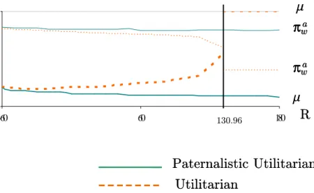
Simulations also allow the emphasis of another situation where monitoring is suboptimal and cannot be captured by the …rst-order conditions. Under the utilitarian criterion, when the exoge-nous resourcesRbecome very high (and larger thanmandwHaccording to all of our simulations),

monitoring becomes suboptimal. Figure 1 illustrates this withm= 2. Under utilitarianism, moni-toring becomes suboptimal whenR 130:96. AtR= 130:96, there is a discontinuity in the prob-ability of type II errors , which jumps up to1. The proportion of able workers, w

a, then sharply

shrinks. And there is a discontinuity in w

a atR= 130:96(see Figure 1). Intuitively, since the

disu-tility terms a reduces the utilitarian welfare level, it is optimal that more and more able workers

stop working whenRincreases. Under paternalistic utilitarianism, our simulations never report a thresholdRbeyond which monitoring is suboptimal. Taking large ranges of(s; R; wL; wH; Nd; m)

(such that monitoring is optimal), we variedRbut never found any case where monitoring became suboptimal. Intuitively, able people who stop working reduce e¢ ciency without improving equity under the paternalistic criterion. Therefore, under paternalism, the proportion of able people who

Paternalistic Utilitarian

Utilitarian

R

m

m

π

π

Paternalistic Utilitarian

Utilitarian

R

m

m

π

π

π

π

Figure 1: Optimal probability of type II error and proportion of able workers as functions ofR.

work, w

a, is stable (see Figure 1 wherem= 2) withR. Financial incentives and monitoring are

both used to keep w

a high and stable. When governmental resourcesR increase, Type II errors

are reduced. They decrease from20% to10%whenR increases from 60to180.

7

Conclusion

This paper assumed an economy where lazy able people may pretend to be disabled and where some disabled people may not take up disability bene…ts designed for them. It has been shown that modeling the monitoring technology and the participation decisions (participation in the labor market and in disability programs) is critical to designing the optimal tax schedule. Formulas for optimal taxation and optimal monitoring accuracy have been provided under paternalistic utilitarian and utilitarian preferences. It has been shown that expensive monitoring supports the use of an Earned Income Tax Credit. We have also discussed how introducing some endogenous take-up cost (as in Besley and Coate, 1992) modi…es the optimal tax formula.

This paper has also shown that when monitoring is costless, perfect monitoring is not optimal. In other words, some cheating is always optimal. Our simulations have shown the quantitative sensitivity of the optimal level of type II errors.

A

Proofs of Propositions 1 and 5

The Lagrangian states as

$=SX+ Nd Z 1 0 [`( d) (wL xwL( d)) (1 `( d))xuL( a)]dF( d) +Na Z 1 0 [`( a) (wH xwH( a)) (1 `( a))xuH( a)]dG( a) R ,

where is the (nonnegative) Lagrangian multiplier associated with the budget constraint. We discuss the paternalistic utilitarian case …rst (i.e., X = P), and show how the properties of the

utilitarian case (X =U) follow.

For any pair( d; a), the …rst-order conditions with respect to the four consumption functions

can be written as:

`( d) [v0(xwL( d)) ] = 0

(1 `( d)) [v0(xuL( d)) ] = 0

`( a) [v0(xwH( a)) ] = 0

(1 `( a)) [v0(xuH( a)) ] = 0

Since `( y) (y = d; a) is equal to 1 or 0, only two of these …rst-order conditions matter. For

those that matter, the corresponding social marginal utilities of consumption have to be equal. For the other two, the consumption function does not matter (as nobody with this value for y is

receiving it). Therefore, since is a constant, we have that the …rst-order conditions with respect to consumption reduce to₈( d; a):

v0(xw_L( d)) =v0(xuL( d)) =v0(xwH( a)) =v0(xuH( a)) =

()x=xw_L( d) =xuL( d) =xwH( a) =xuL( a); (17)

From (17), the tax/transfer toward the disabled workers,x wL, is lower than the transfer to

the inactive disabled,x. A NIT is optimal. From the budget constraint, we have

x=NdwL Z 1 0 `(d )dF(d ) +NawH Z 1 0 `( a)dG( a) +R (18)

x only depends on the number of disabled and the number of able agents who are employed. Consequently, the value of our objective function becomes

v NdwL Z 1 0 `( d)dF( d) +NawH Z 1 0 `( a)dG( ) +R Nd Z 1 0 `( d) ddF( d)

The value of our objective function is maximal when all able agents work: `( a) = 18 a. Therefore,

from the budget constraint, we have x=NdwLR₀1`(d )dF(d ) +NawH+R. Further, as drises

from 0 to ₁, the function `( d) d, where `( d) = 18 d, goes from 0 to 1. Hence, among the

disabled, it will always be optimal to have those in work with the lowest d. Consequently, the

function`( d)will have the following shape: `( d) = 1 for all d bd and`( d) = 0 otherwise.

The critical value is determined by

v0(x)NywYf by Nybyf by = 0

,by =v0(x)wY >0; (19)

with(y; Y) = (d; L). Sincev0_(x)andw

L are …nite,bd<1. It implies that it is optimal for some

disabled individuals not to work.

Under utilitarian preferencesSU_{, it is easy to see that the same …rst-order conditions as under}

ease the notations. From the budget constraint, we then have (18). Substituting (18) inSU _gives

the value of utilitarian welfare as a function of the`( d)and`( a)functions:

v NdwL Z 1 0 `( d)dF( d) +NawH Z 1 0 `( a)dG( ) +R Nd Z 1 0 `( d) ddF( d) Na Z 1 0 `( a) adF( a):

Keeping the number of employed of both types …xed, it is only through the terms on the last line that the shape of the `( d) and `( a) functions matter under utilitarianism. Hence, as k

(k=d; a) rises from0to ₁, the function`( k) k, where `( k) = 18 k, goes from0 to1. Then

it is always optimal to have those in work with the lowest k(k =d; a). Therefore, the functions

`( d)and`( a)have the following shape: `( d) = 1 for all d bd, otherwise zero and`( a) = 1

for all a ba, otherwise zero. Both critical values satisfy (19) with (y; Y) = (d; L)and (a; H),

respectively. Di¤ering from the optimum under the paternalistic criterion, sincev0_{(x)andwH are}

…nite, we now haveba<1, i.e., there are able agents who do not work and receive bene…ts. From

wH> wL and (19),ba>bd as under paternalism.

B

Proof of Equation (1)

By contrast, suppose xH < xL. All able individuals who work choose to produce wL units and

receive net incomexL. From (2) and (3), nobody getsxHas a consumption bundle. Then, keeping

xL…xed, we can assumedxH>0such thatxH+dxH=xL:Now, able people who work produce

wH units and get xH as a consumption bundle. Increasing the level of xH up to xL does not

require any additional consumption sincexH+dxH xL= 0and sinceeaand the number of able

people who work is unchanged. The number of able people who apply for and take up bene…ts is then also unchanged. Hence, from (3), ed and the number of disabled taking up assistance does

not change as well. Yet, all able workers now choose high-skilled jobs and earnwH(> wL). Since

the cost in terms of supplementary consumption is zero and the di¤erence wH wL is strictly

positive, a net receipt appears: wH wL>0. The …scal pie increases and more redistribution can

occur. This will indubitably increase welfare. Therefore, it cannot be optimal for the government to letxL> xH and, thus, consumption when producing more units must be larger: xH xL.

C

At the optimum, all detected able claimants go back to

work: Proof

Proof. Assume lim

x!0v(x) = 1. Able agents choose eitherv(xH) a or, with a probability ,

v(xu₎

a and with a probability 1 , M axfv(xH) a; v(T)g, whereT is a welfare bene…t.

The ICC on able agents states

v(xH) ea= v(xu) + (1 )

h

M axnv(xH) ea; v(T)

oi

Since a is not valued by the Paternalistic Utilitarian criterion and because e¢ ciency matters, 8 a 2[0;1), it is optimal that v(xH) a v(T). This is the famous “principle of maximum

deterrence”. Therefore, sincexH>0, the maximum penaltyT = 0is optimal and all caught able

people go back to work. Therefore, the ICC on able people can be written as (2).

Boadway and Cu¤ (1999) distinguish between the voluntarily and involuntarily non-employed. In their model, when the government perfectly identi…es the voluntary unemployed, the maximum penalty of zero consumption is assumed. In this model, the maximum penalty to the voluntarily inactive able people implies that they do go back to work.

D

Proof of Lemma 1

Proof. (1) Both ea anded are smaller than 1. As 8 a : g( a)> 0 (8 d : f( d) >0), all able

(disabled) people work meansea! 1(ed ! 1) at the optimum. Since consumption levels (and

( u

a)) are …nite, from (2) and ((3)),ea anded cannot tend to1.

(2) If no one works, i.e., ea =ed = 0, it is optimal for everyone to have the same consumption:

xl=xh =xb =R0 withR0 def

M ax_f0; R_g. This allocation will not be optimal if those with the least were to choose to work for the additional consumption equal to their marginal product. It will be the case since v(R0_{+wY) > v(R}0_{) Y = L; H. This implies that}e_{d > 0 (}e_{a > 0) at}

the optimum. More generally, for all planners with an objective function that is increasing in individual utilities, making some disabled work is optimal.

E

Proof and heuristic interpretation of Proposition 2

This appendix derives the necessary conditions of Theorem (2) and gives heuristic interpretations.

First-order condition with respect to xL, (12)

From the Lagrangian, the …rst-order condition with respect toxL gives w d v0_(x L) 1 = (wL xL+xb+M( )) @ w d @xL : (20)

Using (6) and (8), this necessary condition can be rewritten as (12).

A simple heuristic interpretation follows. Consider a small increase in consumption xL (e.g., a

small reduction of the income tax in low-skilled jobs), around the optimal tax schedule. There are a mechanical e¤ect and a behavioral (or labor supply response) e¤ect.

Mechanical e¤ ect

There is a mechanical decrease in tax revenue equal to w_ddxLbecause disabled workers havedxL

additional consumption. This mechanically increases social welfare of disabled workers by their marginal social welfare weightv0_(x

L)= ( gL). Thus, the mechanical welfare gain (expressed in

terms of the value of public funds) as a result ofdxLis equal to(v0(xL)= ) wddxL. Therefore, the

total mechanical e¤ect is w

d (v0(xL)= 1)dxL.

Behavioral e¤ ect Behavioral responses imply a gain in tax revenue. The changedxL >0 induces

@ w

d=@xL (pivotal) disabled workers to enter the labor force. Each worker leaving disability

assis-tance induces a gain in government revenue equal towL xL+xu+M( ). That is the tax paid

disabled recipient (xu_{), as well as the associated cost of monitoring (M( )). The total behavioral}

gain is equal to(wL xL+xu+M( )) (@ wd=@xL)dxL.

At the optimum, the sum of the mechanical and behavioral e¤ects equals zero and gives (20).

First-order condition with respect to xH, (13)

Consider a small change dxH > 0. This change implies mechanical and behavioral e¤ects on

government revenue and welfare.

Mechanical e¤ ect

There is a mechanical decrease in tax revenue equal to w

adxH because able workers consume an

additionaldxH. This mechanical decrease in tax revenue, however, is valued(v0(xH)= 1) wadxH

by the government since each Euro not raised increases the consumption of able workers and this consumption gain is socially valuedv0_{(xH)= ( gH) in terms of public funds.}

Behavioral e¤ ect

There are two e¤ects (direct and indirect) on government revenue as a result of behavioral responses followingdxH >0.

(1) A direct behavioral response comes from@ w

a=@xH (pivotal) previously inactive able agents

who enter the labor force. Each recipient entering the labor force induces a gain in tax revenue of

wH xH+xu, i.e., the tax paid by each new able worker (wH xH) and the bene…t that stops being

paid to him/her. There is also a gain in monitoring expendituresM( )for the (@NaG ea =@xH)

able people who stop applying for disability bene…ts. The gain in government expenditures is then

(wH xH+xu+M( )= ) (@ wa=@xH)dxH. The change dxH also induces a welfare gain since

there are @ w

a=@xH new pivotal workers whose aversion to work ea is not valued in the welfare

function. Valued in terms of public funds, this welfare gain is ea= (@ wa=@xH)dxH. (2) The

previous direct behavioral e¤ect implies an externality e¤ect through the change in the take-up disutility: the changedxH indirectly induces@ wd=@xH pivotal disabled recipients to change their

occupational choice as a result of stigma e¤ects. Using the envelope theorem, (2) and (3), we have @ w

d=@xH >0 (<0) if @ =@ea >0 (<0). Each disabled recipient entering the labor force

induces a revenue gain of wL xL+xu+M( ) for the government. Hence, the total gain is

(wL xL+xu+M( )) (@ wd=@xH)dxH. The change dxH also a¤ects welfare through a change

in the take-up cost’s intensity of the u

d disabled recipients. This change in terms of public funds is

valued u

d(@ =@xH= )dxH by the government. Then, all indirect e¤ects implied by the stigma

(or snowball take-up cost) externality whendxH >0are denoted by (xH; xL; xu; ), de…ned in

Proposition 2.

At the optimum, the sum of the mechanical and all of the behavioral e¤ects has to be nil, which gives: w a v0_(xH) 1 u d @ @xH +ea@ w a @xH = (21) wH xH+xu+ M( ) @ w_a @xH (wL xL+xu+M( )) @ w_d @xH :