Efficient estimation and forecasting in dynamic factor models with structural instability PRELIMINARY AND INCOMPLETE - COMMENTS WELCOME

(1)

Efficient estimation and forecasting in dynamic factor

models with structural instability

PRELIMINARY AND INCOMPLETE - COMMENTS

WELCOME

Dimitris Korobilis† University of Glasgow Christian Schumacher‡ Deutsche Bundesbank June 10, 2014 Abstract

We develop efficient Bayesian estimation algorithms for dynamic factor models with time-varying coefficients and stochastic volatilities for the purpose of monitoring and forecasting with possibly large macroeconomic datasets in the presence of structual breaks. One algorithm can approximate the posterior mean, and the second algorithm samples from the full joint parameter posteriors. We show that our proposed algorithms are fast, numerically stable, and easy to program, which makes them ideal for real time monitor-ing and forecastmonitor-ing usmonitor-ing flexible factor model structures. We implement two forecastmonitor-ing exercises in order to evaluate the performance of our algorithms, and compare them with traditional estimation methods such as principal components and Markov-Chain Monte Carlo.

Keywords: dynamic factor model; time-varying parameters; volatility; variance discount-ing; forgetting factors; forecasting

JEL Classification: C11, C32, C52, C53, C66

This paper represents the authors’ personal opinions and does not necessarily reflect the views of the Deutsche Bundesbank.

†_{Corresponding author. Address: Department of Economics University of Glasgow, Gilbert Scott}

build-ing, University Avenue, Glasgow, G12 8QQ, United Kingdom. Tel: +44 (0)141 330 2950, e-mail:

[email protected]

(2)

1 Introduction

The severity of recent financial crises and the strong contagion and interconnection between modern globalized economies, has lead economists to be interested in two major econometric exercises: the monitoring and analysis of the large amount of information provided in hun-dreds of macroeconomic and financial indicators; and the timely identification, estimation and forecasting of structural breaks and permanent shocks that can hit the economy. In the recent literature, dynamic factor models (DFMs) have been an influential empirical approach in dealing with the former issue1. In fact, the relevant literature is so vast and all sorts of dy-namic factor models have been developed: to extract leading indicators (Stock and Watson, 1989); to forecast using large datasets (Stock and Watson, 2002); and to measure monetary policy using hundreds of variables (Bernanke, Boivin and Eliasz, 2005). At the same time the issue of structural breaks has been very important in all aspects of time-series research, es-pecially for forecasting (Stock and Watson, 1996). Observation of episodes such as the Great Inflation, the Great Moderation and, of course, the recent Great Recession, have sparked a renewed interest for flexible econometric modelling. Therefore, given the turbulent times we live in, it is no surprise that both academics and researchers in central banks have been work-ing over the past decade predominantly with models with driftwork-ing coefficients and stochastic volatilities, that can capture a wide range of nonlinearities and structural breaks; Cogley and Sargent (2001), Sims and Zha (2006), and Primiceri (2005) are a few influential examples of flexible macroeconometric modelling.

In this paper we develop efficient Bayesian estimation methods for time-varying parame-ter dynamic factor models. That is, we estimate unobserved factors coming from a dynamic factor model under a general and flexible form of structural breaks in the coefficients and volatilities. Our ultimate purpose is to accomplish in one comprehensive setting both needs of modern macroeconomists, i.e. to forecast with large datasets while accounting for struc-tural instabilities. In that respect, we follow the standard practice in the macroeconomics literature over the past four decades and we work with DFMs which allow all parameters to drift at each point in time (Cogley and Sargent, 2005). Our paper adds to a vastly expand-ing recent literature arguexpand-ing in favour of structural instabilities in the loadexpand-ings, coefficients, and/or volatilities of dynamic factor models; see Banerjee et al. (2008), Del Negro and Otrok (2008), Stock and Watson (2009), Breitung and Eickmeier (2011), Eickmeier, Lemke and Mar-cellino (2011), Bates, Plagborg-Møller, Stock and Watson (2013), Cheng, Liao and Schorfheide (2013), Corradi and Swanson (2013), Korobilis (2013). However, the major contribution of this paper is that we develop algorithms for numerically stable and computationally efficient estimation of DFMs with time-varying parameters, that make monitoring and recursive fore-casting using large macroeconomic datasets a feasible task.

We propose an estimation algorithm based on the concepts forgetting and variance dis-counting (Koop and Korobilis, 2013), which strike the balance between estimation accuracy and computational tractability in different ways. We propose a two-step estimation proce-dure which is simulation-free and can allow fast updating of the time-varying parameters as well as the factors and is appropriate for high dimensional factor models (e.g. with 100+

1_{The only exception being the analysis of “large vector autoregressions” (Canova and Ciccareli, 2009; Banbura,}

(3)

variables). We examine a simple case where we replace all time-varying covariance matrices with point estimates, and extend to the case where we fully incorporate uncertainty around the time-varying covariances. We show that computation is tractable, with zero probability of programming error or numerical instability occuring even when estimating the TVP-DFM with nonstationary data. We show that we don’t have to impose any of the usual unrealistic identification and normalization restrictions that are regularly adopted in likelihood-based estimation of factor models; see Del Negro and Otrok (2008) and Korobilis (2013). Finally, we provide extensions of our algorithms in several directions which, with the cost of higher com-putational demands, can provide more accurate approximation to the posterior distribution of the time-varying coefficients and covariances.

While it is not obvious how to establish theoretical properties of estimators under very general TVP-DFM structures (see, for instance, the relevant discussion in Bates et al., 2013), we first establish using Monte Carlo experiments that using both our proposed algorithms we can estimate factors which are more accurate than principal components when the true data generating process is a DFM with structural instabilities. We also show that our algorithms are much more computationally stable than popular Markov Chain Monte Carlo (MCMC) algorithms for estimating models with time-varying parameters (Cogley and Sargent, 2005; Del Negro and Otrok, 2008).

In order to show the diverse benefits of the two proposed estimators, we use two datasets which admit a typical factor structure, but which also have very different characteristics in terms of the number of variables, number of time-series observations, and intensity of (ex-pected) structural instabilities in the loadings. In the first empirical application we show the benefits of the three-step estimator in a recursive forecast exercise for German GDP. The fac-tors are estimated from a large data set consisting of quarterly observations on 123 variables observed over the period 1978Q2-2013Q3 thus expanding on the factor forecast results based on PC factors in Schumacher (2007). We show that the factor forecasts from the TVP-DFM provide lower mean-squared forecast errors compared to principal components forecasts. An analysis of the sources of improvements reveals that it is mostly time variation in volatil-ity that matters most, whereas time variation in factor VAR parameters play no role. In the second empirical application we show the benefits of the proposed Monte Carlo sampling algorithm by extracting a single common factor from sovereign bond spreads for 10 Euro-zone countries (base country is Germany) for the period 1999M1-2012M12. This is a typical example of variables which comove together, and are subject to successive, massive struc-tural breaks in the second half of the sample. We use the posterior distribution of the factor and the time-varying parameters and volatilities in order to obtain the full predictive density of the nonlinear spreads series. We show as well that the TVP-DFM estimated with Monte Carlo sampling gives at least 50% higher predictive likelihoods compared to estimates from a time-invariant DFM estimated with MCMC methods.

In the next section we present the general TVP-DFM structure we assume, and discuss the details and characteristics of each of the two proposed algorithms. We also provide details about the nature of the forecasting setting that is more appropriate for each algorithm. Section 3 evaluates estimation accuracy of both algorithms using Monte Carlo simulations. Section 4 demonstrates the superior forecasting performance obtained by estimating a TVP-DFM as opposed to a DFM with constant parameters estimated with principal components, MCMC or

(4)

the two-step estimator of Doz et al. (2011). Section 5 concludes and discusses the implication of this paper for further research.

2 The DFM with time-varying parameters

Our starting point is the standard factor model with factor VAR dynamics, which we extend by allowing all coefficients and volatilities to be time-varying. Letxtbe anp 1 “large” vector of data, then the model we analyze takes the following form

xt = λtft+εt, (1)

ft = Btft 1+η_t, (2)

where ft is the k 1 vector of factors, λt is the p k factor loadings, Bt is a k k matrix of VAR(1) coefficients2_{, and}_ε

t and η_t are disturbance terms. In line with the vast majority

of the macroeconomic literature we assume that εt N(0,Vt), where Vt is a p p diag-onal3 covariance matrix, and η_t N(0,Qt), where Qt is a k k covariance matrix. As-suming that the initial condition of ft is zero, then this model indirectly implies that ft

N 0,(Ik BtL) 1Qt(Ik BtL) 10 . We assume that theεt are uncorrelated with either ftor

η_tat all leads and lags.

This model is quite general to allow for any kind of nonlinearities and/or structural in-stabilities that might occur in λt and β_t. Granger (2008) has formalized this argument and

showed that by specifying parameters to change each time period, we can approximate com-plex forms of nonlinearities in our data. Finally, the DFM with structural instabilities also nests the typical time-invariant parameter DFM, when we restrict variation in all parameters. What is missing so far from the time-varying parameter DFM is to define how the co-efficients evolve, as well as properly define their initial conditions. We do this in the next subsections. Since we are dealing with a very rich model, for the sake of clarity in the next two subsections we separate our presentation into the specification and estimation of the time-varying parameters[λt,ft,β_t], and the specification and estimation of the time-varying

covariances [Vt,Qt]. Then in the next Section we discuss feasible algorithms for combined estimation of all model parameters, discuss their features, their computational feasibility, and the identification of this large model.

2.1 Specificication and estimation of time-varying coefficients

The coefficientsλtandβ_tevolve as driftless random walks of the form

λt = λt 1+νt, (3)

β_t = β_t ₁+υt, (4)

2_{We assume for simplicity a VAR(1) structure with no intercept term just for notational simplicity. This}

shouldn’t cause any concern since every higher-order VAR admits a VAR(1) representation.

3_{This not be the case in approximate factor models, where}_V

t can allow forsomecorrelation. Since we are

interested in likelihood-based estimation, we follow Lopes and West (2004) and others who assume a diagonal covariance matrix.

(5)

whereβ_t = vec(B0_t), andνt N(0,Rt)andυt N(0,Wt)are iid errors, uncorrelated with each other as well asεtandη_tat all leads and lags. This is a standard assumption in the vast

majority of the macroeconomics literature at least since Cooley (1971); see Koop and Korobilis (2010) for a review.

Starting with[λt, ft,β_t], in order to simplify their estimation we note that the model can be

divided into three simple conditionally linear state-space models: Conditional on estimates of the factors, equations (1) and (3) solely contain the loadingsλtas a state variable, whereas equations (2) and (4) solely haveβ_tas the state variable. Conditional on all model parameters,

includingλt andβ_t, equations (1) and (2) form a linear state-space model with state variable ft. As long as the errors in all equations are uncorrelated with each other, sequential esti-mation of each state variable conditional on all other parameters and data (e.g. using the EM algorithm or the Gibbs sampler), is quite natural and can provide an exact, consistent approxi-mation to the joint posterior of the states[λt,ft,β_t]. However, exact estimation using iterative

algorithms such as the Gibbs sampler is subject to identification and numerical problems4_,

and computation becomes nearly infeasible when considering recursive forecasting.5

Therefore our first approximation is to consider estimating [λt,ft,β_t] sequentially from

conditionally linear state-space models, but not necessarily within a (Markov Chain) Monte Carlo scheme. We expand on this issue later in the next section. At this point it is worth not-ing that as we are dealnot-ing with linear state-space models, the Kalman filter is an integral part of our estimation approach. However, in our model, we have to estimate large state covari-ance matrices, which makes it necessary to stabilize the Kalman filter estimation numerically. In our model it is the case that Rt andWt can be of massive dimensions6 and thus their ac-curate estimation using standard likelihood-based formulas (e.g. based on the residual sum of squares) is questionable. The information in the data might not be sufficient to accurately estimate these covariance matrices, or their eigenvalues might become high and conflict infmation in our prior or historical data; see Kulhavý and Zarrop (1993) for more details. In or-der to deal with this issue we follow Koop and Korobilis (2013) and several others, and allow

Rt andWt to be proportional to the filtered covariance matrices ofλt 1jxt 1 andβ_t ₁jxt 1,

respectively, where xt = (x1, ...,xt)denotes all the data information available at time t. If we define the covariance matricesPλ

t 1jt 1 = cov λt 1jxt 1 and P

β

t 1jt 1 = cov βt 1jxt 1 ,

which are readily available from the Kalman filter at timet, we have

Rt = µ₁1 1 P_tλ₁_j_t ₁, (5)

Wt = µ₂1 1 P_tβ _1j_t ₁, (6)

where 0 < µ₁,µ₂ 1 areforgetting factors which allow to discount past data more. Notice

that Pλ

t 1jt 1andP

β

t 1jt 1 are readily available at timetfrom the Kalman filtering algorithm.

4_{See for instance the discussion in Del Negro and Otrok (2008).}

5_{The full model can be viewed as a nonlinear state-space model with state}

θt = [λt,ft,β_t]which can be

esti-mated using nonlinear filters such as the Extended Kalman Filter or the Uncented Kalman Filter; see Koopman et al. (2010). We have found both techniques highly unstable in the presence of the (possibly) large dimension of the loadings matrixλt.

6_{For instance, if we consider empirical applications such as the one by Stock and Watson (2005) with 132}

(6)

Koop and Korobilis (2012, 2013) explain in detail why this is a good approximation and how to interpret and estimate the forgetting factorsµ₁,µ₂. The Kalman filter with forgetting factor

can be used both in adaptive filtering, as well as when using simulation. Details of the Kalman filter and smoother in the presence of forgetting are given in the Appendix.

2.2 Specification and estimation of time-varying covariance matrices

One can typically specify multivariate stochastic volatility models for the covariances as Del Negro and Otrok (2013), or multivariate GARCH models as in Sentana and Fiorentini (2001). Such specifications of the volatilities will typically rely on computationally intensive Monte Carlo sampling methods or complex numerical optimization procedures. Our proposal for feasible estimation of the covariance matrices relies on two estimators.

Exponentially Weighted Moving Average:In the first case we follow Koop and Korobilis (2013) and we assume that Vt andQt are not random variables. Given initial values V0 = diag(V)andQ0 = Q, we obtain point estimates ofVt andQt from exponentially weighted moving average (EWMA) filters of the form

b

Vt = δ1Vbt 1+ (1 δ1)diag bεtbε0_t , (7)

b

Qt = δ2Qbt 1+ (1 δ2)bη_tbη0_t, (8)

wherebεt, and bη_t are residuals in the measurement and state equations at timet, and 0 < δ1,δ2 1 are decay factors giving increasingly more weight to recent data the lower their

values are.

Wishart matrix discounting: In the second case, given priorsV0 iG(S,v) and Q0 iW(Ψ,n), we use Wishart matrix discounting (WMD) models (West and Harrison, 1997) of the form Vt iW(St,nt), (9) Qt iW(Ψt,vt), (10) wherent =δ1nt 1+1 andSt = 1 nt 1 St 1+nt 1 h S1/2_t ₁Ve_t 1/2₁ diag bεtbε0_t Ve_t 1/2₁ S1/2_t ₁ i ,vt = δ2vt 1 +1 and Ψt = 1 vt1 Ψt 1+vt 1 h Ψ1/2 t 1Qet 1/21 bηtηb0tQet 1/21 Ψ1/2t 1 i . In the equations aboveiW denotes the inverse wishart distribution with meanE(Vt) =St/(nt 2)and har-monic meanE V_t 1 1= St/(nt+p 1)(similarly forQt). Details on how to compute the matricesVet 1andQet 1are derived in the appendix.

Both estimators discount older observations faster as δ1,δ2 get lower, by placing more

weight on the current (timet) squared idiosyncratic componentsεtε0_tand residualsη_tη0_t. This

feature might not be so clear for the Wishart matrix discounting case, but after marginalizing e

Vt 1 we can show that the point prediction forVt is equivalent to the EWMA estimator (see Windle and Carvalho, 2013, for a proof).

(7)

3 Algorithms for combined model estimation: computation,

stabil-ity, and model identification

3.1 A simple two-step, one iteration algorithm

We can now examine how to implement combined estimation of all model parameters. Here we build on the work of Koop and Korobilis (2014), as well as Doz et al. (2011, 2012). In partic-ular, we can obtain a recursive solution for the time-varying parameters and the time-varying covariances using a single iteration of the different filters from timet = 1, ...,T, without the need to rely on simulation. In order to achieve this we note that for both the EWMA and the WMD we need to compute the timetresidualsbεt andbη_t based on the equations (1) and

(2), respectively. Of course, these residuals need to be computed for any other likelihood-based estimator of the covariance matrix, e.g. an OLS estimator of the covariance or stochas-tic volatility. Our approximation entails that once we observe data at timetwe estimate the covariance matrices using the Kalman filter prediction errors which are defined as

bεt = xt λ_t_j_t ₁ft, (11)

b

η_t = ft Btjt 1ft 1, (12)

conditional on preliminary factor estimates. The prediction errors are easy to compute, since at time t we are using the known values λ_t_j_t ₁ and β_t_j_t ₁ = vec B_t0

jt 1 instead of the

un-kown λt and β_t. Once these residuals are calculated, we can update Vt,Qt which allows straighforward update ofλt,β_t using the Kalman filter. Therefore, using this approximation

to obtaining the timetresiduals and with the assistance of our simple recursive EWMA and WMD estimators for the covariance matrices, we can define a simple two-step estimator in the spirit of the two-step estimator that Doz et al. (2011) have proposed in the constant parameter DFM. The full algorithm involves the following steps:

Algorithm 1: Two-step, one iteration

0. Obtain the principal component estimate of the factors f_tPC, and initialize all parameters

(λ0,β₀,V0,Q0)

1. Estimate(λt,β_t)and(Vt,Qt)using the Kalman filter and smoother with forgetting and covariance discounting conditional on ft = ftPC

(a) Fort=1, ...,T

EstimateVtbased on the residualbεt =xt λb_t_j_t ₁ft, andQtbased on the resid-ualbη_t = ft Bbtjt 1ft 1using either the EWMA or the WMD estimators

Updateλtandβ_tgivenVt,Qt,xt, and ft

(b) Fort= T, ..., 1 run a typical (e.g. a fixed interval) smoother

2. Estimate ft using the Kalman filter and smoother, where all parameters of the state-space model are known from the previous steps

(8)

The algorithm described above has several advantages. Estimation is quite simple since we need to run once three Kalman filters - one for each conditionally linear state-space model - and not iterate over these steps thousands of times as in MCMC algorithms. The recur-sive estimators for the covariances are also computationally efficient. Thus we can have an estimate in seconds even for the most demanding models. Most importantly, identification of the factors is guaranteed, at least to the level that identification of principal components is guaranteed, see Bai and Ng (2013). We can explain this very important issue intuitively. First, notice that the time-varying parameters and covariances in step 1 are estimated condi-tional on the PC estimates of the factors, that is the factors are given in our information set. Additionally, there is no identification issue between time-variation in the mean (λt,β_t) and

time-variation in the covariances (Vt,Qt) of each of the DFM equations. This is a feature which results from the approximation of the timetresiduals using the parameters λb_t_j_t ₁,bβ_t_j_t ₁

in-stead of the unkown . As a result, we can estimateVt,Qtconditional on quantities which are all known at timet, and then subsequently updateλt,Bt given timetestimates of the time-varying covariances. Then in a recursive manner, at time t+1 we follow exactly the same procedure, until we reach the last observation.7

Finally, we need to note that the procedure described above can be used for both the point (EWMA) and full Bayesian (WMD) estimators of the covariance matricesVt and Qt. In the case of the EWMA estimator this is straightforward, since it immediately provides a single value for the covariance matrices. For the WMD we obtain a full posterior distribution for these covariance matrices. Therefore, in light of avoiding the need to simulate from this posterior using computationally intensive Monte Carlo methods, we can simply feed the har-monic mean estimatesE V_t 1 1 = St/(nt+p 1)andE Q_t1

1

= Ψt/(vt+k 1)into the Kalman filter.

3.2 Extensions of the basic framework

In computationally demanding big-data applications, such as forecasting GDP or inflation using large panels with more than 100 macroeconomic variables (Stock and Watson, 2002) or constructing factors from vast dimensional covariance matrices of returns, the algorithm presented above provides a feasible approach to estimating the parameters of the TVP-DFM. In other applications which involve smaller datasets, the algorithm above can be modified to provide higher estimation precision. We discuss here such possibilities.

First, notice that for the WMD estimator, the algorithm above does not allow to obtain samples from the joint posterior of the time-varying parameters and covariances. As we show

7_{Note that smoothing, i.e. running backward recursions to obtain estimates at time}_t_{given information at time}

t+s,s>0, can be implemented using exact formulas, since it only depends on having estimates of all parameters from the forward recursions. In our algorithm we are using the Kalman smoother because we find it very useful in getting more precise estimates. Nevertheless, use of the Kalman smoother is not necessary if one wishes to pursue online estimation and forecasting. In this case only the forward iteration of the Kalman filter can be used, and there is no need to re-estimate the model from time 0 every time we want to forecast (in which case, the gains in computation are massive). See Koop and Korobilis (2012) for an example.

(9)

in the appendix, these joint posteriors are of the form

λt,Vt N IW λ_t_j_T,P_tλ_j_T,S_t_j_T,v_t_j_T , β_t,Qt N IW β_t_j_T,P_tβ_j_T,Ψ_t_j_T,n_t_j_T .

whereN IWdenotes the Normal-Inverse-Wishart distribution, and exact details of the hyper-parameters are given in the Appendix. In this case, we can use Monte Carlo Integration to obtain samples from this distribution which involves iteratively samplingVtfrom an inverse Wishart distribution, and then samplingλtfrom a Normal distribution conditional onVt. We can proceed similarly forβ_t,Qt. This procedure can provide samples from the approximate posterior of the model parameters. Conditional on these, we can use the simple Kalman fil-ter/smoother or the simulation smoother (Carter and Kohn, 1994) to obtain samples from the posterior distribution of the factors.

Another possibility is to iterate steps 1 and 2 of our basic algorithm where in the second iteration and beyond we can estimate (λt,β_t)and(Vt,Qt)conditional on the estimate of ft from the previous step. The resulting Expectation Conditional Maximization (Gelman, Carlin, Stern and Rubin, 2004) resembles the EM algorithm extension proposed by Doz et al. (2012). There are advantages and disadvantages of implementing this approach. On the one hand, we can possibly get better a approximation of the posterior, e.g. if we iterate multiple times we not only condition on ft from the previous iteration, but we can also calculate the residuals bεt and bη_t using estimates of λ_t_j_T and β_t_j_T from the previous iteration.8 On the other hand,

there is no guarantee that the system is identified. In this case we need to use identification and normalization restrictions in order to properly identify the factors and the time-varying parameters. Zero restrictions are typically applied in the loadingsλt and covariancesQtand

Vt, as in Geweke and Zhou (1996) and Aguilar and West (2000). Alternatively, some initial conditions can be fixed instead of being considered random, e.g. settingλ0=0 instead of the

diffuse priorλ0 N(0, 100); see Del Negro and Otrok (2008) for more information on this

issue. Additionally, when iterating this algorithm mutliple times we need to have a stopping rule (e.g. converge of the likelihood to a fixed value), which is guaranteed theoretically but is not always practically feasible, especially in high-dimensional dynamic factor models.

4 Simulations

In this Section we carry out a small Monte Carlo study to numerically evaluate the perfor-mance of the algorithms to accurately track the true factors coming from a DFM with para-meters that evolve as random walks. In particular, we generate artificial observations for the following data generating process which broadly follows Banerjee, Marcellino and Masten

8_{We remind that in the one-iteration case, these parameters are replaced with}

λtjt 1 and β_t_j_t ₁ which are

(10)

(2008) and Bates et al. (2013) xit = λitft+V1/2_i e_it, λit = λit 1+ (c )eit, λi0 N(0,a), a U(0, 1) ft = Btft 1+Q1/2et, Bt =β_tIk, β_t = β_t ₁+ dT 1 et, β₀ = b.

wherei= 1, . . . ,Nandt = 1, . . . ,T, andetdenote standard Normal disturbances which are of appropriate dimensions for each equation they appear. In such a rich specification there are many choices that need to be made. First, we simplify the structure of the covariance matrices9 in the factor and VAR equations () and (), respectively, by assuming that V_i U(0, 1)and Q = diag q

1, ...,qk where qj U(0, 1) for all j = 1, ...,k. This assumption allows us to focus on the actual effect of time variation in the parameters λt and β_t on the

final factor estimates. We also setb=0.5 andd=0.4.

The crucial parameter in our simulation is the one controlling the amount of time-variation in the loadings10_{, i.e. the parameter}_c _{. We specify three different values of}_c _which

corre-spond to slow, medium and fast changes in λit 8i. For the slow and medium variation we follow Bates et al. (2005) and specifyc = cT 3/4 with c = 2 and 3.5, respectively. For the faster time-variation we setc =4.5T 3/4_.

For all simulation results we generate from the above DFM data generating process with one factor and one lag, and we respectively estimate models with one factor (and one lag when not using principal components). Our interest lies on factor estimation, therefore, we do not implement model selection and assessment of misspecification. For application of de-terministic and stochastic model selection techniques using predictive likelihoods the reader is referred to Koop and Korobilis (2013) and Korobilis (2013), respectively. Estimation accu-racy is assessed with theSFF0 statistic which is defined as

SFF0=

tr f₀0bf fb0bf bf0f0 tr(f₀0f0)

,

where f0is the true factor and bf is the estimated factor. SFF0 is standardized to have values

between zero and one, with one meaning that the estimated factors completely fit the true factors.

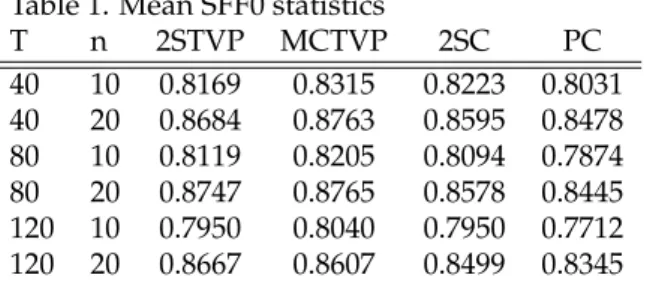
First we implement a simulation exercise with small T and n, in order to assess both the fast two-step estimator and the computationally more demanding Monte Carlo estima-tor. Table 1 presents mean SFF0 statistics when generating combinations of small DFMs with

9_{Basically, the results presented here do not change qualitatively if we instead generate diagonal covariance}

matrices following geometric random walks (stochastic volatility model).

10_{We have found that time-variation in the persistence of the factors (}

β_t) is not of paramount importance for

factor estimation, at least compared to time-variation in the loadings (λt). This finding is in-line with the Monte Carlo results of Banerjee, Marcellino and Masten (2008, Section 3.4).

(11)

T = 40, 80, 120 and n = 10, 20. The columns present results for our two-step estimator with known covariance matrices (2STVP), the Monte Carlo estimator (MCTVP), the 2-step estima-tor of Doz et al. (2011) for the constant parameter DFM (2SC), and the principal components nonparametric estimator (PC).

Table 1. Mean SFF0 statistics

T n 2STVP MCTVP 2SC PC 40 10 0.8169 0.8315 0.8223 0.8031 40 20 0.8684 0.8763 0.8595 0.8478 80 10 0.8119 0.8205 0.8094 0.7874 80 20 0.8747 0.8765 0.8578 0.8445 120 10 0.7950 0.8040 0.7950 0.7712 120 20 0.8667 0.8607 0.8499 0.8345

In Table 2 we generate a set of models with larger time-series and cross-sectional dimen-sions, using combinations of T = 50, 100, 200, 500 andn = 50, 100, 200, 500. Here we only assess the 2STVP estimator versus Doz et al. (2011) and the principal components.

(12)

T able 2. Mean SFF0 statistics c = 5 T 3 / 4 c = 3.5 T 3 / 4 c = 2 T 3 / 4 T N 2STVP 2SC PC 2STVP 2SC PC 2STVP 2SC PC 50 50 0.9085 0.8820 0.87 82 0.8971 0.8880 0.8795 0.8870 0.8915 0.8784 50 100 0.8905 0.8553 0.85 15 0.9089 0.8992 0.8875 0.8992 0.9057 0.8885 50 200 0.8678 0.8372 0.83 27 0.9056 0.9002 0.8856 0.9257 0.9314 0.9137 50 500 0.8447 0.8255 0.82 13 0.9254 0.9225 0.9053 0.9350 0.9403 0.9199 100 50 0.9157 0.8889 0.88 70 0.9155 0.9020 0.8962 0.9085 0.9088 0.9003 100 100 0.8965 0.8621 0.859 8 0.9204 0.9068 0.8992 0.9362 0.9368 0.9262 100 200 0.8755 0.8436 0.841 5 0.9285 0.9211 0.9108 0.9469 0.9506 0.9384 100 500 0.8514 0.8301 0.828 4 0.9399 0.9396 0.9269 0.9651 0.9686 0.9551 200 50 0.9191 0.8909 0.88 98 0.9282 0.9128 0.9095 0.9346 0.9316 0.9262 200 100 0.9008 0.8651 0.864 2 0.9336 0.9189 0.9135 0.9468 0.9463 0.9384 200 200 0.8793 0.8462 0.845 1 0.9418 0.9346 0.9271 0.9622 0.9638 0.9546 200 500 0.8551 0.8338 0.832 6 0.9535 0.9537 0.9437 0.9713 0.9741 0.9651 500 50 0.9192 0.8914 0.89 09 0.9293 0.9140 0.9120 0.9393 0.9324 0.9292 500 100 0.9023 0.8675 0.867 1 0.9363 0.9202 0.9162 0.9575 0.9544 0.9494 500 200 0.8799 0.8480 0.847 7 0.9465 0.9389 0.9330 0.9651 0.9651 0.9589 500 500 0.8544 0.8343 0.833 8 0.9591 0.9594 0.9518 0.9801 0.9823 0.9763 Note: Results ar e based on 2000 generated d atasets fr om the homoskedas tic DFM with time-varying p arameters described in the m ain text. The two-step estim ator of the DFM with time-varyin g parameters is denoted as 2S TVP . Results fr om the two-st ep estimator of the constant parameter DFM (Giannone, R eichlin and Sala, 2005) ar e in the columns labelled 2SC. Fin aly , SFF0 statistics based on p rincipal components ar e in the columns labelled PC.

(13)

5 Assessment based on real data

In this section we evaluate empirically the performance of each of the two algorithms using two datasets which are quite different in nature and call for a different treatment using factor methods. The first one is a typical forecasting exercise where the target is to forecast GDP using a large macroeconomic panel of hundreds of stationary variables. In the second empir-ical analysis we use factor methods to extract a common component from a small number of nonstationary financial variables (bond yields), and our purpose is to forecast the variables themselves. We show that there are potential forecasting benefits for considering a nonlinear factor specification versus using principal components, and we also provide solid evidence that our estimation methodology is more stable than Markov Chain Monte Carlo (MCMC) estimation of the TVP-DFM.

5.1 Forecasting using large panels

The first empirical exercise evaluates factor forecasts for German GDP growth with recent data including the Great Recession. The recursive forecast simulation is in the spirit of Stock and Watson (2002). The large data set consists of quarterly observations on 123 variables ob-served over the period 1978Q2-2013Q3. The data is taken from Pirschel and Wolters (2014) and represents an updated version of the data used in Schumacher (2007), where PC factor forecasts have been addressed. The time series used here are described in detail in the appen-dix of Schumacher (2007).

The initial sample period starts in 1978Q2 and ends in 2002Q2. Given that sample, the factor models are estimated, forecasts derived and stored. Then, the end of the sample period is expanded by one quarter, and the forecasts are repeatedly computed. We end up with a sequence of forecasts and forecast errors. As a summary statistic, we compute the mean-squared forecast error (MSE). In the Tables below, we report the MSE of a factor model relative to the MSE of a benchmark AR model. The key competitor to the TVP-DFM is the diffusion index ARDL model by Stock and Watson (2002). We use forecast equations with up to four factors. The AR and lag order of the factors is specified using the BIC, which is applied recursively with a maximum lag order of four.

To estimate the TVP-DFM, we employ the two-step algorithm from Section 2.1 given the large size of the data set. To estimate drifting volatilities we em,ploy both EWMA and WMD. To specify the model, we consider up to four factors. Initial conditions are diffuse:

f0 N(0k 1, 4 Ik), vec(λ0) N(0nk 1, 4 Ink),V = In,Q = cov(f_tPC)for volatilities, and

β₀has a Minnesota prior as in Koop and Korobilis (2013). Note that the covariances ofλ0and β₀also initialize Rt andWt, respectively, in (5) and (6). We also have to specify the variance discounting parameters: The forgetting factorsµ₁andµ₂reflect the different degrees of time

variation in the loadings and VAR polynomial parameters, respectively. δ1andδ2 determine

the time variation in the volatility of idiosyncratic components and factor VAR residuals. Thus, we can choose between different combinations of time variation and volatility. To ex-plore which of these potentially different sources of time variation matter most with respect to forecasting accuracy, we choose a large grid of the discounting factors and the number of factors. In particular, we compare 900 model specifications, whereµrange from 0.96 to 1.00,

(14)

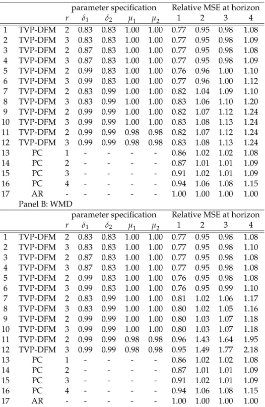
The forecast results for a subset of good models are summarized in Table 2 with EWMA drifting volatilities in Panel A and with Wishart matrix discounting in Panel B. We report forecasts for horizons up to four.

(15)

Table 2: Relative MSE for forecasting German GDP growth Panel A: EWMA

parameter specification Relative MSE at horizon

r δ1 δ2 µ₁ µ₂ 1 2 3 4 1 TVP-DFM 2 0.83 0.83 1.00 1.00 0.77 0.95 0.98 1.08 2 TVP-DFM 3 0.83 0.83 1.00 1.00 0.77 0.95 0.98 1.09 3 TVP-DFM 2 0.87 0.83 1.00 1.00 0.77 0.95 0.98 1.08 4 TVP-DFM 3 0.87 0.83 1.00 1.00 0.77 0.95 0.98 1.09 5 TVP-DFM 2 0.99 0.83 1.00 1.00 0.76 0.96 1.00 1.10 6 TVP-DFM 3 0.99 0.83 1.00 1.00 0.77 0.96 1.00 1.12 7 TVP-DFM 2 0.83 0.99 1.00 1.00 0.82 1.04 1.09 1.10 8 TVP-DFM 3 0.83 0.99 1.00 1.00 0.83 1.06 1.10 1.20 9 TVP-DFM 2 0.99 0.99 1.00 1.00 0.82 1.07 1.12 1.24 10 TVP-DFM 3 0.99 0.99 1.00 1.00 0.83 1.08 1.13 1.24 11 TVP-DFM 2 0.99 0.99 0.98 0.98 0.82 1.07 1.12 1.24 12 TVP-DFM 3 0.99 0.99 0.98 0.98 0.83 1.08 1.13 1.24 13 PC 1 - - - - 0.86 1.02 1.02 1.08 14 PC 2 - - - - 0.87 1.01 1.01 1.09 15 PC 3 - - - - 0.91 1.02 1.01 1.09 16 PC 4 - - - - 0.94 1.06 1.08 1.15 17 AR - - - 1.00 1.00 1.00 1.00 Panel B: WMD

parameter specification Relative MSE at horizon

r δ1 δ2 µ₁ µ₂ 1 2 3 4 1 TVP-DFM 2 0.83 0.83 1.00 1.00 0.77 0.95 0.98 1.08 2 TVP-DFM 3 0.83 0.83 1.00 1.00 0.77 0.95 0.98 1.10 3 TVP-DFM 2 0.87 0.83 1.00 1.00 0.77 0.95 0.98 1.08 4 TVP-DFM 3 0.87 0.83 1.00 1.00 0.77 0.95 0.98 1.08 5 TVP-DFM 2 0.99 0.83 1.00 1.00 0.76 0.95 0.98 1.08 6 TVP-DFM 3 0.99 0.83 1.00 1.00 0.76 0.95 0.99 1.10 7 TVP-DFM 2 0.83 0.99 1.00 1.00 0.81 1.02 1.06 1.17 8 TVP-DFM 3 0.83 0.99 1.00 1.00 0.80 1.02 1.05 1.16 9 TVP-DFM 2 0.99 0.99 1.00 1.00 0.80 1.03 1.07 1.18 10 TVP-DFM 3 0.99 0.99 1.00 1.00 0.80 1.03 1.07 1.18 11 TVP-DFM 2 0.99 0.99 0.98 0.98 0.96 1.43 1.64 1.95 12 TVP-DFM 3 0.99 0.99 0.98 0.98 0.95 1.49 1.77 2.18 13 PC 1 - - - - 0.86 1.02 1.02 1.08 14 PC 2 - - - - 0.87 1.01 1.01 1.09 15 PC 3 - - - - 0.91 1.02 1.01 1.09 16 PC 4 - - - - 0.94 1.06 1.08 1.15 17 AR - - - 1.00 1.00 1.00 1.00

(16)

(rows 13-16) can outperform the AR benchmark (row 17) forh = 1, but not at longer hori-zons. The best TVP-DFM can outperform the benchmark up to three quarters, complementing existing results on the limits of GDP growth forecastability in Germany in Schumacher (2007). Generally, TVP-DFM with two or three factors do best. Compared to PC factor forecasts, most of the displayed TVP-DFM perform better at all horizons in terms of relative MSE (rows 1-6). In particular, TVP-DFM do best mainly due to the volatility in the factor VAR residuals, as

δ2=0.83 leads to better forecast compared toδ2=0.99, (compare rows 1-6 to 7-12) . Volatility

in the idiosyncratic components does not seem to have a huge impact given the factor VAR residual volatility withδ2=0.83 (compare rows 1-6): settingδ1=0.83,δ1 =0.87 orδ1 =0.99

yields quite similar forecast results. Setting very slow moving volatilititesδ1 = δ2 = 0.99

(rows 9-10) leads to a decline in forecast accuracy at all horizons, such that the forecasts are uninformative compared to the benchmark forh=2, 3. Time-varying loadings or VAR para-meters cannot improve the forecasts. Specifying very slow moving volatilititesδ1 =δ2 =0.99

and moderate timne variation in the loadings and VAR parametersµ₁ = µ₂ = 1.00 worsens

the forecast performance considerably (rows 11-12). The best models haveµ₁ = µ₂ = 1.00,

implying no time variation at all. But overall, we find that variations in the volatility seems to matter most for forecasting, see also Eickmeier, Marcellino and Lemke (2013).

If we compare results between Panel A with EWMA volatilities and Panel B with WMD, we see no sharp differences. The best models with WMD seem to perform slightly better than the corresponding EWMA models.

5.2 Forecasting sovereign bond yields

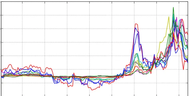
Another dataset which has an evident factor structure, is subject to structural changes, and which has attracted much attention during the post-2009 Eurozone debt crisis, involves 10-year sovereign bond yields as spreads from the 10-10-year yield of the German bund. We collect data for ten Eurozone countries, namely Austria, Belgium, Finland, France, Greece, Ireland, Italy, Netherlands, Portugal, and Spain, for the period 1999m1-2012m12. This is a small panel of countries, and we have relatively short time series dimension for being in the monthly fre-quency. However, there are evident breaks in these data as shown in Figure XXXX: around the end of 2008 there is an explosion of volatility due to the Global financial crisis. The Eurozone crisis starts around the end of 2009, exacerbates in mid-2010 with Greece being on the verge of a default, and abruptly peaks around mid 2011 and early 2012 (depending on the country).

(17)

2000M09 2002M05 2004M01 2005M09 2007M05 2009M01 2010M09 2012M05 -2 -1 0 1 2 3 4 5

Figure 1. Returns on 10-year bond for 10 Eurozone countries, 1999m1-2012m12. The data are expressed as spreads from the 10-year yield of the German bund, and then standardized

(mean zero, variance one) in order to be of comparable scale.

While the relevant literature either identifies one factor or two factors, i.e. a so-called “core” factor (Austria, Belgium, Finland, France, Netherlands) and a “periphery” factor (GI-IPS), we prefer to adopt a single-factor approach in order to focus on the properties of dif-ferent estimators without having to worry for the moment about uncertainty regarding the number of factors11. What is more important here is that we are dealing with a nonstationary dataset. Despite having a variable expressed as a spread, the time-series process is explosive. Interestingly this implies that simple principal component analysis in nonstationary data is equivalent to estimating a sample mean: indeed, with few exceptions, the loadings of the first principal component from this dataset, degenerate to 1, thus implying that the PC is an equally weighted average. Maximum likelihood estimation of the factor model can provide a possibly more accurate solution in this case, and assign varying weights to the estimate of the factor.

Therefore, we estimate the TVP-DFM using the two recursive estimators we have pro-posed in this paper, and we contrast these to MCMC estimation of the TVP-DFM with ran-dom walk stochastic volatility of the form introduced in Kim, Shephard and Chib (1998). For the purpose of forecasting we are also estimating using MCMC a time-invariant DFM with diffuse priors. The reader is referred to the Appendix for details regarding specification and estimation of the TVP-DFM with stochastic volatility, and the simple, constant parameter DFM. In the Appendix we also make an additional empirical assessment of the accuracy of the different methods in recovering the time-varying volatilities and the factors. What we present here analytically is the settings we have used for each model. We do that in Table XX,

11_{While the tradition is to choose the number of factors using some criterion, the Bayesian forecaster can simply}

use a model selection prior (e.g. SSVS), a shrinkage priors (e.g. Bayesian LASSO), or a model averaging prior (Zellner’s g-prior); see Koop and Korobilis (2010) for more details of priors and acronyms.

(18)

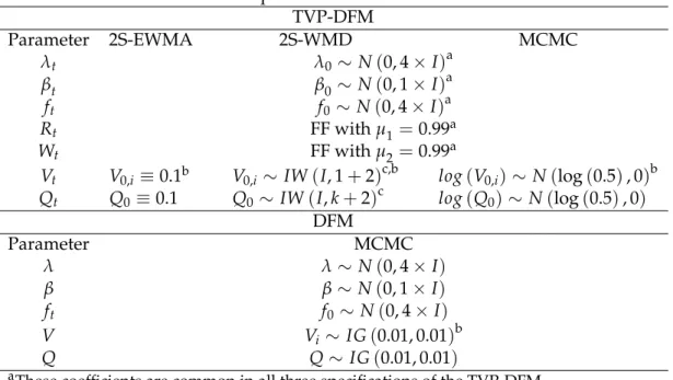
where the reader can see that wherever possible we are using diffuse priors, plus we are us-ing the same priors (initial conditions) for all parameters which are common among different model specifications.

Table XX. Initial conditions and priors used in different models TVP-DFM Parameter 2S-EWMA 2S-WMD MCMC λt λ0 N(0, 4 I)a β_t β₀ N(0, 1 I)a ft f0 N(0, 4 I)a Rt FF withµ₁ =0.99a Wt FF withµ₂ =0.99a Vt V0,i 0.1b V0,i IW(I, 1+2)c,b log(V0,i) N(log(0.5), 0)b Qt Q0 0.1 Q0 IW(I,k+2)c log(Q0) N(log(0.5), 0) DFM Parameter MCMC λ λ N(0, 4 I) β β N(0, 1 I) ft f0 N(0, 4 I) V Vi IG(0.01, 0.01)b Q Q IG(0.01, 0.01)

a_{These coefficients are common in all three specifications of the TVP-DFM}

b_V

0,i(similarly,Vi) denotes thei-th diagonal element ofVt(similarly,V),i=1, ..., 10.

c_{The IW for a univariate variable is equivalent to the Inverse Gamma (IG) distribution.}

What we need to keep from this Table is that the major differences in the three estimators of the TVP-DFM occur in the specification of the volatility. For these parameters we can be fairly noninformative when using the Wishart matrix discounting method (2S-WMD), but we have to be very informative for the other two methods. For the EWMA specification ofVt and Qt our prior (initial condition) is informative, since it is just a scalar initial value. For the MCMC estimation we can define a starting value from the Normal distribution, however, for identification reasons we have to normalize12 the volatilities to start from a fixed point which explains why our prior variance is zero. We need also to note that for identification of the factors we normalize the first element of λt to be 1 (and, hence, not time-varying); see Del Negro and Otrok (2008) for an explanation why such restrictions are needed. In the 2S-EWMA and 2S-WMD specifications, according to our discussion in Section XX, we need not use any normalization or identification restrictions to obtain the common factor so that estimation and numerical converegence is always guaranteed.

Regarding the forecast evaluation using the three estimation methods of the TVP-DFM, we calculate posterior predictive likelihoods13 which means that we need to use posterior

12_{For forecasting we presumably can ignore identification issues (at least, when we are referring to}

identi-fication of the factors), however, allowing less informative priors for the log-volatilities can have catastrophic consequences for forecast uncertainty.

13_{The posterior predictive likelihood is obtained by evaluating the whole predictive density obtained from}

(19)

simulation (Monte Carlo) to obtain samples from the predictive density. Note that with the MCMC we have by definition Monte Carlo samples from the posterior of all parameters, and eventually the predictive density. The esitmated predictive likelihoods are presented in Table X below. These are quoted relative to the predictive likelihood of a Bayesian time-invariant DFM estimated using diffuse (noninformative) priors.

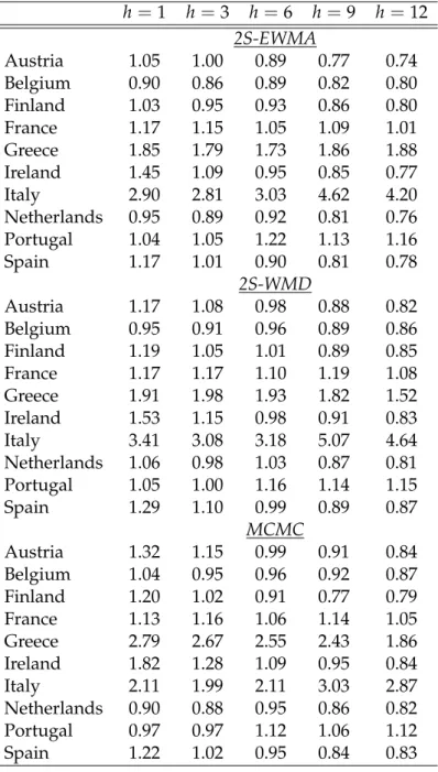
Table X. Relative PL’s for the bond yield data

h=1 h=3 h=6 h=9 h=12 2S-EWMA Austria 1.05 1.00 0.89 0.77 0.74 Belgium 0.90 0.86 0.89 0.82 0.80 Finland 1.03 0.95 0.93 0.86 0.80 France 1.17 1.15 1.05 1.09 1.01 Greece 1.85 1.79 1.73 1.86 1.88 Ireland 1.45 1.09 0.95 0.85 0.77 Italy 2.90 2.81 3.03 4.62 4.20 Netherlands 0.95 0.89 0.92 0.81 0.76 Portugal 1.04 1.05 1.22 1.13 1.16 Spain 1.17 1.01 0.90 0.81 0.78 2S-WMD Austria 1.17 1.08 0.98 0.88 0.82 Belgium 0.95 0.91 0.96 0.89 0.86 Finland 1.19 1.05 1.01 0.89 0.85 France 1.17 1.17 1.10 1.19 1.08 Greece 1.91 1.98 1.93 1.82 1.52 Ireland 1.53 1.15 0.98 0.91 0.83 Italy 3.41 3.08 3.18 5.07 4.64 Netherlands 1.06 0.98 1.03 0.87 0.81 Portugal 1.05 1.00 1.16 1.14 1.15 Spain 1.29 1.10 0.99 0.89 0.87 MCMC Austria 1.32 1.15 0.99 0.91 0.84 Belgium 1.04 0.95 0.96 0.92 0.87 Finland 1.20 1.02 0.91 0.77 0.79 France 1.13 1.16 1.06 1.14 1.05 Greece 2.79 2.67 2.55 2.43 1.86 Ireland 1.82 1.28 1.09 0.95 0.84 Italy 2.11 1.99 2.11 3.03 2.87 Netherlands 0.90 0.88 0.95 0.86 0.82 Portugal 0.97 0.97 1.12 1.06 1.12 Spain 1.22 1.02 0.95 0.84 0.83

From the table above we can make the following observations

(20)

1. There is a strong case for using a DFM with structural instabilities for the Eurozone data, compared to a constant parameter DFM. Short-run predictability is greatly improved by the presence of stochastic volatility and time-variation in loadings and VAR coefficients. This is more evident, as one would expect, for countries in the periphery such as Italy and Greece.

2. Our proposed estimation methods compare as well in achieving similar predictive like-lihoods to MCMC. In some cases the TVP-DFMs we have estimated with the two-step algorithms have lower PLs than MCMC, but in a several cases they improve the fit of the model a lot (e.g. in the case of Italy for the 2S-WMD algorithm).

3. We should also consider in this evaluation that the Monte Carlo versions of our two-step algorithms are several times faster than MCMC.14 Additionally, we haven’t imposed any identification restrictions to obtain our results. This is not the case for the MCMC algorithm, where identification is far more challenging. More discussion on this is pro-vided in Appendix B.

4. Our algorithms can also be extended in several directions. For example, the results above suggest that for some countries (e.g. Belgium) a TVP-DFM might not be appro-priate, and one might be better-off with a constant parameter DFM. Similar results have been found in the macro-finance literature, e.g. Sims and Zha (2006) show that the op-timal specification for a monetary VAR is one that allows coefficients to change only in the interest rate equation (and be constant in the other equations in their system). If we allow each DFM equation to have a different forgetting factor forλt, that is, if we make

µ₁a diagonal matrix instead of a scalar, we can allow some countries to have constant

loadings while others to have time-varying.

5. In a similar spirit, one can optimize the model in terms of all the forgetting and decay factors used. Windle and Carvalho (2013) use a Metropolis-Hastings step to optimize the respective decay factors in their model, however, adopting such an approach means that we lose the simplicitly of using our two-step approach and we instead have to adopt a more complex MCMC scheme in order to obtain the EWMA and WMD estimates. Koop and Korobilis (2013) and Dangl and Halling (2012) use an alternative method where they define a grid of values for their decay/forgetting factors, and they chose as the optimal model the one that maximizes the timetpredictive likelihood.

There several such extensions along the lines of points 4 and 5 above, which could be exciting ideas for future research. In this paper we avoid to go in such depths, as our purpose is to establish that the proposed algorithms work with a minimal amount of tunning. For example, if we optimize with respect to the forgetting/decay factors, then it is not clear if the benefits of our estimation approach come from the simplicity of the algorithm or because of the fact that we are taking into account uncertainty about the amount of time variation in the DFM system.

14_{Exact times depends on the programming language, machine hardware, and number of Monte Carlo}

itera-tions. Indicatively we mention here that it takes exactly 1/5 of the time to obtain 5,000 iterations from the 2S-WMD algorithm compared to the MCMC algorithm (in a PC with “typical” specifications, i.e. a Core i7 4770K machine, running Windows 7 with MATLAB 2013a 64-bit installed).

(21)

6 Conclusions

In this paper, we develop fast and efficient Bayesian estimation algorithms for dynamic factor models with time-varying coefficients and stochastic volatilities. The models can be estimated on large macroeconomic datasets and are well-suited for real-time monitoring and forecast-ing. We propose two variants of the estimation procedure: One algorithm can approximate the posterior mean and tackle very large data sets, and the second algorithm samples from the full joint parameter posteriors, is therefore computationally a bit more demanding and thus suited for medium-sized data sets.

In simulations, we show that our proposed algorithms are fast and accurate in the pres-ence of structural breaks. We also carry out two forecasting exercises to illustrate the prop-erties of the estiamtors further: The first exercise aims at forecasting German GDP growth recursively given a dataset of more than hundred time series. The other exercise addresses the predictablity of government bond spreads in the Euro area countries. Both exercises cover the recent period as evaluation period, a period which was subject to severe financial turbu-lences and a an unprecedented break-down in real economic activity. In these periods, we can show considerable advantages of the time-varying model in forecast performance over models, which do not allow for structural instabilities.

(22)

References

[1] Aguilar, O. and West, M. (2000). “Bayesian dynamic factor models and portfolio alloca-tion,”Journal of Business & Economic Statistics, 18, 338-357.

[2] Bai, J. and Ng, S. (2013). “Principal components estimation and identification of static factors,”Journal of Econometrics, 176, 18-29.

[3] Banerjee, A., Marcellino, M. and Masten, I. (2008). Forecasting macroeconomic variables using diffusion indexes in short samples with structural change. CEPR Discussion Pa-pers 6706, C.E.P.R. Discussion PaPa-pers.

[4] Bates, B. J., Plagborg-Møller, M., Stock, J. H. and Watson, M. W. (2013). “Consistent factor estimation in dynamic factor models with structural instability,”Journal of Econometrics, Available online 17 April 2013, doi: 10.1016/j.jeconom.2013.04.014

[5] Brauning, F. and Koopman, S. J. (2012). “Forecasting macroeconomic variables using col-lapsed dynamic factor analysis,” Tinbergen Institute Discussion Papers 12-042/4, Tin-bergen Institute.

[6] Breitung, J. and Eickmeier, S. (2011). “Testing for structural breaks in dynamic factor models,”Journal of Econometrics163(1), 71-84

[7] Cheng, X., Liao, Z. and Schorfheide, F. (2013). “Shrinkage estimation of dynamic factor models with structural instabilities,” University of Pennsylvania.

[8] Corradi, V. and Swanson, N. R. (2013). “Testing for structural stability of factor aug-mented forecasting models,”Journal of Econometrics, forthcoming.

[9] Cogley, T. and Sargent, T. J. (2005). “Drift and volatilities: Monetary policies and out-comes in the post WWII U.S,”Review of Economic Dynamics, 8(2), 262-302.

[10] Dangl and Halling (2012). “Predictive regressions with time-varying coefficients,” Jour-nal of Financial Economics106(1), 157–181.

[11] Del Negro, M. and Otrok, C. (2008). “Dynamic factor models with time-varying para-meters: measuring changes in international business cycles,” Staff Reports 326, Federal Reserve Bank of New York.

[12] Doz, C., Giannone, D. and Reichlin, L. (2011). “A two-step estimator for large approx-imate dynamic factor models based on Kalman filtering,” Journal of Econometrics, 164, 188-205.

[13] Doz, C., Giannone, D. and Reichlin, L. (2012). “A quasi–maximum likelihood approach for large, approximate dynamic factor models,” Review of Economics and Statistics, 94, 1014-1024.

[14] Eickmeier, S., Lemke, W. and Marcellino, M. (2011). “The changing international trans-mission of financial shocks: evidence from a classical time-varying FAVAR,” Deutsche Bundesbank, Discussion Paper Series 1: Economic Studies, No 05/2011

(23)

[15] Frale, C. , Marcellino, M., Mazzi, G. L. and Proietti, T. (2011). “EUROMIND: a monthly indicator of the euro area economic conditions.” Journal of the Royal Statistical Society Series A, 174, 439-470.

[16] Gelman, A., Carlin, J. B., Stern, H. S. and Rubin, D. B. (2004).Bayesian Data Analysis(2nd ed.). Chapman & Hall/CRC: New York.

[17] Geweke, J. and Zhou, G. (1996). “Measuring the pricing error of the arbitrage pricing theory.”The Review of Financial Studies, 9, 557-587.

[18] Granger, C. W. J. (2008). “Non-Linear Models: Where Do We Go Next - Time Varying Parameter Models?,”Studies in Nonlinear Dynamics & Econometrics, 12, Article 1.

[19] Han, X. and Inoue, A. (2012). “Tests for parameter instability in dynamic factor models,” manuscript North Carolina State University.

[20] Jungbacker, B. and Koopman, S. J. (2008). “Likelihood-based analysis for dynamic factor models,” Tinbergen Institute Discussion Papers 08-007/4, Tinbergen Institute.

[21] Kapetanios, G. and Marcellino, M. (2009). “A parametric estimation method for dynamic factor models of large dimensions,”Journal of Time Series Analysis, 30, 208-238.

[22] Koop, G. and Korobilis, D. (2012). “Forecasting inflation using dynamic model averag-ing,”International Economic Review, 53, 867-886.

[23] Koop, G. and Korobilis, D. (2013). “Large time-varying parameter VARs,” Journal of Econometrics, 177, 185-198.

[24] Koop, G. and Korobilis, D. (2014). “A new index of financial condtions,”European Eco-nomic Review, .

[25] Koopman, S.J., Mallee, M.I.P. and van der Wel, M. (2010). Analyzing the Term Structure of Interest Rates using the Dynamic Nelson-Siegel Model with Time-Varying Parameters.

Journal of Business and Economic Statistics28, 329-343.

[26] Korobilis, D. (2013), “Assessing the transmission of monetary policy using time-varying parameter dynamic factor models”.Oxford Bulletin of Economics and Statistics, 75, 157-179. [27] Kulhavý, R. and Zarrop, M. B. (1993). On a general concept of forgetting.International

Journal of Control58, 905-924.

[28] Nelson, L. and Stear, E. (1976). “The simultaneous on-line estimation of parameters and states in linear systems,”IEEE Transactions on Automatic Control21, 94 - 98.

[29] Prado, R. and West, M. (2010).Time Series: Modeling, Computation, and Inference. Chapman & Hall/CRC: Boca Raton.

[30] Quintana J. M. and West M. (1987). “An analysis of international exchange rates using multivariate DLMs,”Statistician36, 275–281.

(24)

[31] Sentana, E. and Fiorentini, G. (2001). “Identification, estimation and testing of condition-ally heteroskedastic factor models,”Journal of Econometrics, 102, 149-170.

[32] Schumacher, C. (2007). “Forecasting German GDP using alternative factor models based on large datasets,”Journal of Forecasting, 26, 271-302.

[33] Shumway, R. H. and Stoffer, D. S. (1982), “An approach to time series smoothing and forecasting using the EM algorithm,”Journal of Time Series Analysis, 3, 253–264.

[34] Stock, J. and Watson, M. W. (2002). “Macroeconomic forecasting using diffusion in-dexes,”Journal of Business & Economic Statistics, 20,147-162

[35] Stock, J. and Watson, M. W. (2006). “Forecasting using many predictors,” In: Graham Elliott, Clive Granger and Allan Timmerman (Eds), Handbook of Economic Forecasting, North Holland: Elsevier.

[36] Stock, J. and Watson, M. W. (2009). “Forecasting in dynamic factor models subject to structural instability,” In: Jennifer Castle and Neil Shephard (Eds),The Methodology and Practice of Econometrics: A Festschrift in Honour of Professor David Hendry, Oxford: Oxford University Press.

[37] Triantafyllopoulos, K. (2007). “Covariance estimation for multivariate conditionally Gaussian dynamic linear models”,Journal of Forecasting26, 551-569.

[38] West, M. and Harrison, P. J. (1997). Bayesian Forecasting and Dynamic Models(2nd ed.). Springer: New York.

[39] Windle, J. and Carvalho, C. M.(2013). “Forecasting high-dimensional, time varying co-variance matrices for portfolio selection”. manuscript, University of Texas at Austin. [40] Wolff (1987). “Time-varying parameters and the out-of-sample forecasting performance

(25)

A. Technical Appendix

Consider the state space model of the form

yt = Htxt+vt,

xt = xt 1+wt,

where the noise processesvtandwtare white, zero-mean, uncorrelated, and have covariance matricesΣtandΩt, respectively. Here we use a notation where the discount (forgetting) factor ofΩtisλ, and the discount (decay) factor ofΣtisδ. In the next two subsections we show how

to obtain an estimate the statextwhenΣtis known (EWMA estimator) or unknown (inverse Wishart process estimator). Therefore, the filters/smoothers presented below can be used to compute the first step of both algorithms suggested in the text, that is for estimation of the time-varying parameters ofλt andβ_t. The second step in both algorithms (estimation of the

factors ft) is always based on the typical Kalman filter/smoother recursions; see for example Durbin and Koopman (2001).

A.1 Kalman filter and smoother with covariance discounting

For chosen initial conditionsx0,P0,Σ0and discounting factorsλ,δ, and given fixed values for

the system matrices Ht for allt, the algorithm for updating the unkown statext along with the unknown covariancesΣt,Ωt, is as follows

Kalman-EWMA filter

Fort =1, ...,Trun the following recursions

x_t_j_t ₁= x_t _1j_t ₁, predicted mean

Ωt = λ 1 1 P_t ₁_j_t _1, forgetting step P_t_j_t ₁ =P_t ₁_j_t ₁+Ωt, predicted covariance

e

vt = yt Htxtjt 1 , measurement innovation Σtjt =δΣt 1jt 1+ (1 δ)vetev0t, EWMA covariance estimate

Kt =Ptjt 1x0t Σt+xtPtjt 1x0t

1

, Kalman gain

x_t_j_t= x_t_j_t ₁+Ktevt, updated mean

P_t_j_t =P_t_j_t ₁ KtxtPtjt 1. updated covariance Fixed interval smoother

Given xT andPTjT from the last run of the Kalman filter, the fixed interval smoother for

x_t_j_t₊₁,t =T 1, ..., 1, is as follows

x_t_j_t₊₁ = x_t_j_t+U_tx x_t₊₁_j_t₊₁ x_t₊₁_j_t ,

Ptjt+1 = Ptjt+Utx Pt+_1jt+1 Pt+_1jt Utx0,

(26)

A.2 Sequential Bayes learning with covariance discounting Given the initial conditions

x0 N(x0,P0), Σ0 iW(S0,n0),

the timetpriors ofxt,Σtare

xtjyt 1 N xtjt 1,Ptjt 1 , Σtjyt 1 iW Stjt 1,ntjt 1 ,

wherex_t_j_t ₁ =x_t ₁_j_t ₁,P_t_j_t ₁= P_t ₁_j_t ₁+Ωt,Ωt = λ 1 1 P_t ₁_j_t _1,,S_t_j_t ₁ =S_t ₁_j_t ₁, and n_t_j_t ₁=δn_t _1j_t ₁.

Given these priors, the joint timetposterior ofxt,Σtis of the form

xt,Σtjyt N IW xtjt,Ptλjt,Stjt,ntjt ,

where x_t_j_t = x_t_j_t ₁+ P_t_j_t ₁HtΞt 1eεt and Ptjt = Ptjt 1 Ptjt 1Ht0Ξt 1HtPtjt 1, witheεt = yt

Htxtjt 1the innovation error of the Kalman filter andΞt = HtPtjt 1Ht0+Σtits covariance ma-trix. Additionally, we have thatn_t_j_t =δn_t ₁_j_t ₁+1 andS_t_j_t= (1 at)St 1jt 1+at

h S1/2_t ₁ jt 1Ξ 1/2 t 1 (εtε0t)Ξt 1/21 S1/2t 1jt 1 i , withat =nt 1andΞt 1=Σt 1+Ht 1Pt 1jt 1Ht0 1; see also Triantafyllopoulos (2007).

In order to sample fromxt andΣtwe use a Monte Carlo scheme that allows us to sample sequentially fromΣtjytandxtjΣt,yt. However, as we iterate forward over time we also need to iterate backwards to obtain smoothed estimates. Therefore, we first get a draw fromΣtjyt by running the filtering and smoothing recursions, and then we obtain xtjΣt,yt using also filtering and smoothing recursions. In particular, fors =1, ...,Ssamples from the posterior of the parameters of interest, we iterate over the following equations

Obtain a sampleΣtby generating a draw from Σ(s)

t jyt iW StjT,ntjT . (A.1)

In order to obtainS_t_j_T,n_t_j_Twhere we first run the forward recursions fort=1, ...,Tand estimate i) n_t_j_t=δn_t ₁_j_t ₁+1 andS_t_j_t = (1 at)St 1jt 1+at h S1/2_t _1j_t ₁Ξ_t 1/2₁ εtε0_tΞ_t1/2₁ S1/2_t _1j_t ₁ i . and then run the backward recursions fort =T 1, ..., 1 and estimate

ii) n_t_j_T = (1 δ)n_t_j_t+δn_t₊₁_j_T andS_t_j_T1 = (1 δ)S_t_j_t1+δS_t₊1_1j_T

Obtain a samplextby generating a draw from

x(_ts)_jΣ(_ts),ys N x_t_j_T,P_t_j_T . (A.2) In a similar fashion, we first run the forward Kalman filter iterations fort= 1, ...,Tand obtain

(27)

i) x_t_j_t = x_t_j_t ₁+ P_t_j_t ₁Ht Ξ (s) t 1 eεt and Ptjt = Ptjt 1 Ptjt 1Ht0 Ξ (s) t 1 HtPtjt 1 where nowΞ(_ts)= HtPtjt 1Ht0+Σ (s) t .

Subsequently we can run the backward Kalman filter recursions to obtain

ii) x_t_j_t₊₁ =x_t_j_t+U_tx x_t₊₁_j_t₊₁ x_t₊₁_j_t andP_t_j_t₊₁= P_t_j_t+U_tx P_t₊₁_j_t₊₁ P_t₊₁_j_t U_tx0,where

U_tx= P_t_j_t P_t+_1jt

1

.

This sampling procedure makes it trivial to analyze (nonlinear) features of the parameter posteriors (e.g. impulse response functions, or posterior predictive likelihoods), since we can simply then use Monte Carlo Integration; see Koop (2003) for details.

Subseuently, in our second algorithm we use equation (A.1) to sample Vt and Qt, and equation (A.2) to sampleλt andβ_t, given their conditional state-space forms. Note thatVtis diagonal so one can either use the posterior expression (A.1) using the restriction thatStjtand

S_t_j_Tare diagonal matrices, or sample each diagonal element ofVtfrom equivalent univariate inverse Gamma posterior; see West and Harrison (1997) for more details.

B. Additional results

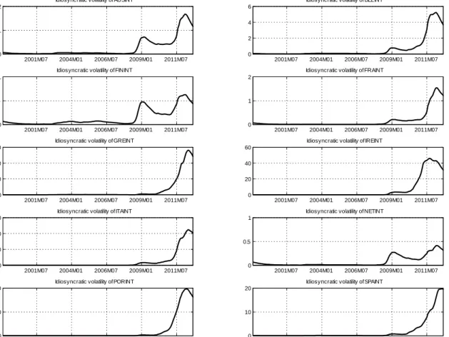
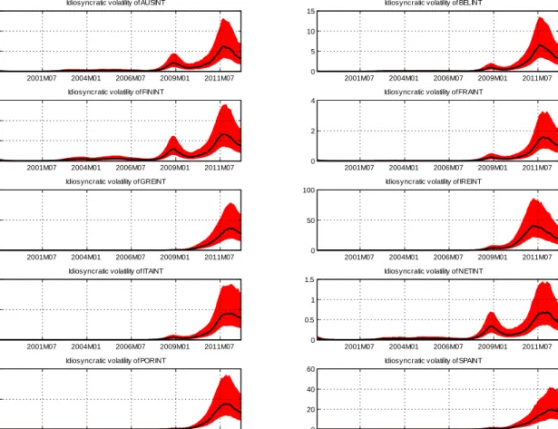
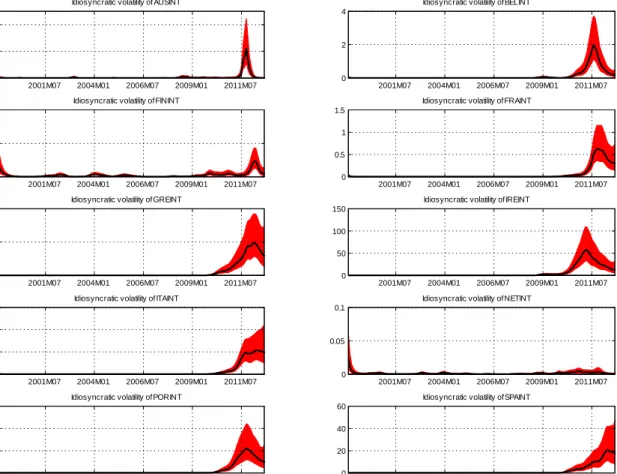
In this section we present evidence on the way our estimation algorithms fit patterns in the data. For the Eurozone bond spreads data we present estimates of the volatilities and factors that pertain to the full sample 1999:M1-2012:M12. Figures B1-B3 present estimates of the idiosyncratic volatilities for each of the 10 countries in the data, which can be found along the main diagonal of the time-varying covariance matrix Vt. Figure B1 corresponds to EWMA point estimates, while Figures B2 and B3 correspond to WMD and MCMC (Gibbs sampler - see Del Negro and Otrok, 2008, for computational details) where posterior medians (solid line) with the 16th and 84th quantile are plotted. These plots of the volatilities show the part of our model which is not due to comovents captured in the common componentλtft, rather they are attributed to the individual characteristics of each country (in the error termεt). This explains why for the peripheral countries (Greece, Italy, Ireland, Portugal, Spain) there is a large part of unexplained volatility15 during the Eurozone crisis 2010-2012, while for core countries (Austria, Belgium, Finland, France, Netherlands) the major spikes in their volatility occurs both during the Eurozone crisis and during the Global crisis 2007-2009

15_{This “unexplained volatility” could potentially be explained by macroeconomic fundamentals such as the}

(28)

Idiosyncratic volatility of AUSINT