Full Terms & Conditions of access and use can be found at
https://www.tandfonline.com/action/journalInformation?journalCode=rero20
ISSN: 1331-677X (Print) 1848-9664 (Online) Journal homepage: https://www.tandfonline.com/loi/rero20
Tangible investment and labour productivity:
Evidence from European manufacturing
Alina Stundziene & Asta Saboniene
To cite this article: Alina Stundziene & Asta Saboniene (2019) Tangible investment and labour productivity: Evidence from European manufacturing, Economic Research-Ekonomska Istraživanja, 32:1, 3519-3537, DOI: 10.1080/1331677X.2019.1666024
To link to this article: https://doi.org/10.1080/1331677X.2019.1666024
© 2019 The Author(s). Published by Informa UK Limited, trading as Taylor & Francis Group
Published online: 25 Sep 2019.
Submit your article to this journal
Article views: 116
View related articles
Tangible investment and labour productivity: Evidence
from European manufacturing
Alina Stundziene and Asta Saboniene
School of Economics and Business, Kaunas University of Technology, Kaunas, Lithuania
ABSTRACT
Labour productivity is one of the key drivers for higher earnings and welfare standards in every economy. The problem of how to ensure the growth of labour productivity is especially relevant to less developed economies and forces justification of the factors affecting sustainable productivity growth. The purpose of this research is to test if the investment in tangible assets improves labour productivity in the European manufacturing industry and to reveal the countries with inefficient investment. The results show that with consideration of all European countries, a 1% increase in gross investment in tangible goods (G.I.T.G.) per per-son employed (P.E.) has a 0.0373% long-run effect on apparent labour productivity (A.L.P.). Considering various types of invest-ments in tangibles, only an increase in gross investment in exist-ing buildexist-ings and structures (G.I.E.B.S.) per P.E. and gross investment in machinery and equipment (G.I.M.E.) per P.E. caused growth of A.L.P. However, the impact of investment in assets on A.L.P. significantly differs among the countries and it is revealed that many European countries, which are characterised by low productivity, use investment inefficiently.
ARTICLE HISTORY Received 14 February 2019 Accepted 29 July 2019 KEYWORDS productivity; labour productivity; investment; tangible investment; manufacturing indus-try; Europe JEL CLASSIFICATIONS D24; D92; J24; L60 1. Introduction
The growth of productivity, which is closely related to sustainable development and eco-nomic prosperity, remains a topical issue in any developed or developing economy. Productivity reflects the efficiency of production, and higher productivity represents the improved competitiveness at both micro and macro levels. Natural resources, techno-logical knowledge, physical and human capital affect the indicators of productivity (Mankiw & Taylor, 2008). The impact of investment in tangibles on productivity remains a relevant problem for scholars and practitioners. This empirical study focuses on the analysis of labour productivity with consideration of the availability of this meas-ure in statistics. Higher labour productivity ensmeas-ures a higher level of wages conditioned by higher outputs gained. The problem of productivity growth has earned much
CONTACTAlina Stundziene alina.stundziene@ktu.lt
ß2019 The Author(s). Published by Informa UK Limited, trading as Taylor & Francis Group.
This is an Open Access article distributed under the terms of the Creative Commons Attribution License (http://creativecommons.org/ licenses/by/4.0/), which permits unrestricted use, distribution, and reproduction in any medium, provided the original work is properly cited.
–
scientific attention, in particular, in terms of the key growth drivers. Considering the indicators of labour productivity in the E.U., a gap between the countries is visible, i.e., lower indicators belong to E.U. countries that are catching up.
The impact of investment on labour productivity is analysed in various theoretical and empirical studies. The common neoclassical approach, which conceptually explains the changes in labour productivity that occur due to the technological progress and the changes in the capital–labour ratio, was suggested by Solow (1956). The Solow model argues that technological change makes labour and capital more productive, and the main assumptions of this neoclassical growth model are an exogenous nature of technological change and labour growth combined with the diminishing marginal product of capital. Some new growth models expanded the analysis of investment by emphasising its endogenous effects on growth and productivity. Baily (1981) research confirmed that labour productivity in the U.S. is correlated with a capital investment in the aggregate, but at the same time revealed some puzzling discrepancies at the industrial level. Stiroh (2000) pointed out that various components of investment are highly correlated in prac-tice, and any attempt to measure the impact of any type of investment on productivity must consider a broad specification with appropriate quality adjustments. According to Ding and Knight (2009), changing technology requires investment, and investment inevit-ably involves technological change.
This article seeks to expand the empirical research on labour productivity factors by focusing on the analysis of the impact of tangible investment on the manufacturing industry. Manufacturing plays a significant role in lots of European countries, and the investment in tangibles is essential to industry. Considering the positive links between investment in tangibles and labour productivity, the policy implications, directed to remove the factors that reduce a company’s willingness and possibility to invest in both the tangible and intangible, to adopt the newest technologies, and maintain significant role to labour productivity growth. If the investment in tangible goods does not contrib-ute to labour productivity, then the growth of tangible investment is groundless and can reflect insufficient utilisation of the investment. It is especially relevant for new members of the E.U., as an obvious gap in their labour productivity can be observed.
The purpose of this research is to test if the investment in tangible goods – such as land, construction and alteration of buildings, machinery and equipment – improves labour productivity in the European manufacturing industry. The research also aims to reveal the countries with inefficient investment. The interdependencies between labour productivity and investments in tangibles have been extensively approached in the litera-ture, but this research views it from a different angle in its aim to expand the empirical literature on this subject. Our contribution to the issue is based on performing a detailed analysis of the impact of different types of tangible investment on labour productivity in E.U. countries and to provide deeper insights on the different effects in countries employing recent data. The emphasis of this research is to find out if the impact of investment in tangibles on labour productivity differ among countries and identify the countries where investment in tangible goods is inefficient.
The research employs the panel data of the European manufacturing industry for 2005–2016. The methods of comparative analysis, correlation analysis, Granger
causality test, vector autoregression (V.A.R.) and panel regression analysis are also employed in the research.
The remainder of this article is organised as follows: the first section covers the theoretical background on apparent labour productivity (A.L.P.) and tangible invest-ment; the second section introduces the methodology of the empirical study; the third section of the article covers the results and findings of the analysis; the final section provides a summary of the results and our main conclusions.
2. Theoretical background
The impact of investment on physical assets, advanced technologies and technological innovations, as well as improvement of human knowledge, skills and abilities, is substan-tiated in previous and recent scholarly literature where the key drivers of efficient pro-duction, high economic value and labour productivity are considered (Black & Lynch, 2001; Shaw,2004). A company’s productivity is assumed to be an increasing function of the cumulative aggregate investment for an industry, while increasing returns rise because new knowledge is considered as investment (Arrow, 1962). According to Stiroh (2000), two common approaches can be discussed when considering the role of invest-ment and productivity in explaining the exogenous and endogenous variables of eco-nomic growth. The first of them is the neoclassical theory suggested by Solow (1956). In the Solow model, technological change is an exogenous variable. Solow argues that an economy with an initially low capital–labour ratio will have a high marginal product of capital, and the gross investment in new capital goods may exceed the amount needed to equip new employees. Capital per employee will rise, and this will generate a decline in the marginal product of capital if returns to scale are constant and a technology is fixed. Solow assumed an aggregate production function as a linearly homogeneous func-tion: Y¼Af(K, L), where Y indicates output, L and K – tangible inputs of labour and capital, and A – a measure of technical change. Following the Solow model, accumula-tion of resources largely depends on productive tangible investment and formaaccumula-tion of gross fixed capital. The expression Y/L¼Af(K/L, 1) means that output per hour worked, that is labour productivity, depends on the rate of per hour capital accumula-tion. The Solow model is based on several assumptions, according to which the growth of an economy would converge to a steady state, and less developed countries would catch up with rich countries. According to Chen et al. (2014), the Solow model’s assumptions of the exogenous technological progress and the decreasing returns to cap-ital remain a controversial issue, and the factors that plausibly affect economic growth are left out (Ding & Knight,2009). Mankiw, Romer, and Weil (1992) suggested a modi-fied model whereby the differences among countries in per capita income should be explained by the variability in physical and human capital investments and labour growth. According to Acemoglu (2008), the Solow model has enough substance to take it to data in total factor productivity accounting, regression analysis and calibration in order to analyse the sources of economic growth over time and of income differences across countries. Acemoglu, however, thinks that no single approach is entirely convinc-ing, and the conclusion, driven from Solow’s accounting framework and proposing that technology is the main source of economic growth, is disputable. Acemoglu (2008) also
points out that sufficient adjustments to the quality of physical and human capital sub-stantially reduce or even totally eliminate residual productivity growth.
The second approach is known as the endogenous growth theory, developed by Romer (1990), Lucas (1988), Rebelo (1991). According to the new concept of endogenous growth, economic growth is primarily the result of endogenous factors. In the long run, the economy that has developed science, capital and human resour-ces will have a larger economic growth rate, while higher investment in human cap-ital, innovation, and knowledge will lead to a larger income per capita growth rate. The contributors to this approach extended the theory of investment by arguing the impact of any accumulated input on labour productivity, while productivity growth was recognised to be encouraged by investment in the factors that could be expanded and improved.
Arguing the manifold effect of investment, Grifell-Tatje and Lovell (2015) noted that the impact of new technologies on productivity depends on the presence of com-plementary inputs (including organisational capital and skilled staff), and stressed that adoption of new technologies may increase both– productivity and competition. New technologies may cut general or specific labour costs. They may also reduce cap-ital needs through, for example, increased utilisation of equipment and reduction in inventories or space requirements. New technologies may also lead to higher product quality or contribute to better product development conditions.
The research on the relations between investment and labour productivity provide different findings. By applying a multilevel regression model, Bini, Nascia, and Zeli (2014) analysed the links between the current level of labour productivity and a set of indicators (including tangible investment) in Italian companies. Their empirical study confirmed that a lag-distributed positive impact of tangible investment on labour productivity really exists. Empirical research ofSwierczynska (2017) justify the role of technology progress to labour productivity in developing countries by implementing institutional policies facilitating investments. Nilsen et al. (2008) argue that productiv-ity improvements are not related to instantaneous technological change through investment spikes. Fare, Grosskopf, and Margaritis (2006) found the evidence that aggregate productivity in different economic sectors may diverge due to the diver-gence of technical change. The economies with access to the same technologies, simi-lar volumes of investment, trade and other rates may differ in their ability to innovate and adopt new technologies. Salinas-Jimenez, Alvarez-Ayuso, and Delgado-Rodriguez (2006), who analysed E.U. data between 1980 and 1997, found that capital accumulation seems to have contributed positively to labour productivity conver-gence. Physical and human capital accumulation appears to be the key driver of labour productivity convergence since a strong inverse link between capital deepening and the initial levels of output per worker is not observed. Salinas-Jimenez et al. (2006) also note that the positive regression slope between output per worker and technological change suggests that advanced economies gain greater benefits from technological progress than less productive economies. Thus, technological progress tends to contribute to the divergence of labour productivity in different countries.
Strobel (2011) examined the sources of labour productivity growth in selected industri-alised countries and showed that the investment in information and communication
technology (I.C.T.) was indeed one of the driving factors. Strobel revealed that the inter-action between I.C.T. and skills spurred the growth of labour productivity, although it was quite heterogeneous within the E.U. Member States. Cette et al. (2016) also note that the use of I.C.T. leads to capital deepening, which, in its turn, boosts labour productivity. Falling I.C.T. prices induce firms to increase their desired capital stock.
Some authors tested the opposite relation, i.e., they analysed how investment depends on productivity. For example, Chaudhuri et al. (2010) developed a model, based on a standard production function of a firm, to test the hypothesis that firms with higher labour productivity were associated with higher investment growth in several manufacturing industries in India. They found that the factors related to cap-ital or labour productivity explain a large amount of variation within the firms. Improved capital and labour productivity can also provide the necessary impetus required for future investment and growth.
In concluding the literature review, it can be stated that the impact of tangible investment on labour productivity is a controversial and not conclusive issue. The results vary due to the different level of economic development, dissimilar rates of tangible investment in different industries, environmental factors and corporate behaviour. This article is designed to provide detailed empirical analysis on which to base the links of investment in tangibles on labour productivity. It also helps us to recognise the differences of effects by employing the manufacturing data of European countries in order to draw the conclusions about the effects of tangible investment on labour productivity in the region.
3. Data and methodology
The standard Solow model is considered and output Ytis defined by the equation:
Yt¼ KtaðAtLtÞ1a, (1)
where Ktis physical capital, At represents the level of technology, Ltis labour, and a
is the capital share in production which is bounded between zero and one. This equa-tion can also be written as follows:
Yt Lt ¼ At Kt AtLt a ¼A1ta Kt Lt a : (2)
Calculation of logarithms respectively allows coming up to the linear regression: ln Yt Lt ¼ð1aÞlnAtþaln Kt Lt : (3)
Equation (3) indicates that A.L.P. increases when capital rises. So the purpose of this research is to find out how the investment in capital per person employed (P.E.) affects A.L.P. in the European manufacturing industry. Various types of investment are under investigation in order to find out which of them have the greatest impact on A.L.P. The types of investment under investigation include gross investment in
tangible goods (G.I.T.G.), gross investment in land (G.I.L.), gross investment in exist-ing buildexist-ings and structures (G.I.E.B.S.), gross investment in construction and alter-ation of buildings (G.I.C.B.), gross investment in machinery and equipment (G.I.M.E.), and net investment in tangible goods (N.I.T.G.).
Several influential factors are also added into the analyses as exogenous variables to gauge the robustness of the baseline correlations and to potentially address further misspecification issues. These include macro and industry related factors, i.e.:
gross domestic product (G.D.P.) at current market prices, euro per capita;
exports of all products, million E.C.U./euro;
turnover per P.E. in manufacturing industries, thousand euro;
average personnel costs (personnel costs per employee) in manufacturing indus-tries, thousand euro.
This empirical study employs the data of the manufacturing industries in 29 European countries for the period 2005–2016. Since the data for 2016 is unavailable for many countries, the data for 2015 is often taken as the latest data for comparative analysis. The data are an unbalanced annual frequency panel, which is balanced between the start and end. The data are obtained from Eurostat.
The research employs the following methods:
correlation analysis which shows how strong the relationship is between A.L.P. and the investment in capital per P.E.;
Granger causality test which defines the delayed effect (lags) and the direction of the relation between labour productivity and investment in capital per P.E.;
panel regression analysis and V.A.R. which give the expression of the relationship between the indicators. V.A.R. can capture the linear interdependencies among multiple variables, so it is useful if the reciprocal relation between variables is observed. Panel regression analysis is employed to test if this relationship between variables varies among the countries.
Granger causality test reveals if x causes y or how much of the current y can be explained by past values of y. This research examines the effect of five previous years (five lags of the variables). Granger causality test is performed assuming that all coef-ficients are the same across all cross-sections.
The relation between A.L.P. and investment in capital per P.E. can also be described by V.A.R. and panel regression models. The models are created according to the results of Granger-causality test, i.e., the significant lags of endogenous and exogenous variables are included into the model. The lag length for the V.A.R. model is determined by using model selection criteria. A sufficiently large number of lags is used when estimating a V.A.R. model. Then the lag length selection test, based on likelihood ratio (L.R.), the Hannan-Quinn criterion (H.Q.), Akaike Information Criterion (A.I.C.) and Schwarz Bayesian Information Criterion (B.I.C.) information criteria, is performed to verify if the same model can be estimated with fewer lags of the variables included. The lag associ-ated with the minimum value of a criterion is selected.
Once a V.A.R. model has been developed, the next step is to determine if the selected model provides an adequate description of the data. Autocorrelation of the residual values based on the Lagrange Multiplier (L.M.) test is used to determine the goodness of fit of the model. Stability refers to checking whether the model is a good representation of how the time series evolved over the sampling period. The esti-mated V.A.R. is stable (stationary) if all the roots have modulus less than one and lie inside the unit circle. If the V.A.R. is not stable, certain results (such as impulse response standard errors) are not valid.
Testing for the existence of any cross-section (individual) or time effects is import-ant in panel regression settings since accounting for the presence of these effects is necessary for the correct specification of the regression and proper inference. Evaluation of cross-section effects shows if there exist any significant changes among countries, while evaluation of time effects reveals whether the relation between A.L.P. and investment in capital per P.E. is influenced by time.
The significance level of 0.05 is employed for all the tests of the hypothesis. Calculations are made by employing Eviews software.
4. Results
4.1. Descriptive statistics of the data
The average A.L.P. of the manufacturing industries in 29 European countries for the period 2005–2016 amounted to e55,000 and varied over a comparatively large inter-val, i.e., from 5 to 442 thousand euro (Table 1). The highest A.L.P. was reached in Ireland where it increased twice during 2015. A.L.P. was also high in Switzerland and Norway. Meanwhile, Bulgaria, Romania, Latvia and Lithuania were distinguished by the lowest A.L.P. with relatively slow improvements. The ratio of A.L.P. in these countries increased twice during the last 10 years.
Although A.L.P. in Germany was not so far from the mean of Europe, Germany was one of the leaders in various types of investment. In 2015 Germany had the high-est values of G.I.T.G., G.I.C.B., G.I.M.E., and N.I.T.G. G.I.T.G. was also high in
Table 1. Summary statistics for the variables.
Variable Mean Median Minimum Maximum Std. Dev. IQ range
Apparent labour productivity (thousand euro)
54.5 48.4 5.0 441.7 47.7 53.7
Gross investment in tangible goods per person employed (thousand euro)
8.3 7.2 2.1 149.3 9.0 4.9
Gross investment in land per person employed (thousand euro)
0.2 0.1 0.0 1.0 0.2 0.1
Gross investment in existing buildings and structures per person employed (thousand euro)
0.5 0.2 0.0 10.5 1.2 0.2
Gross investment in construction and alteration of buildings per person employed (thousand euro)
1.3 1.2 0.0 4.2 0.6 0.7
Gross investment in machinery and equipment per person employed (thousand euro)
5.6 5.1 1.1 18.8 2.9 4.4
Net investment in tangible goods per person employed (thousand euro)
France, Ireland and the U.K. G.I.C.B. as well as G.I.M.E. were also high in the U.K. and Italy. N.I.T.G. was high in Ireland and the U.K., meanwhile it was negative in Italy in 2013.
Switzerland was the leader in G.I.E.B.S. G.I.L. in 2015 was the highest in Italy, Spain and the U.K. Meanwhile, Cyprus, Luxembourg, Estonia and Latvia were among the smallest investors in all types of assets.
As the amount of investment partly depends on the size of the economy, it is use-ful to analyse the relative indicators. Gross (and net) investment in tangible goods per P.E. in 2015 was the highest in Ireland, Belgium and Switzerland. These countries were also the leaders in G.I.E.B.S. per P.E.. Belgium and Switzerland were also the leaders in G.I.M.E. per P.E. A high rate of G.I.M.E. per P.E. in 2015 was observed in Sweden, the Netherlands and Luxembourg.
Luxembourg, as well as Norway and Finland, had the highest G.I.C.B. per P.E. in 2015. Meanwhile, Denmark was the leader in G.I.L. per P.E. It was also high in Belgium, Portugal and Spain.
Cyprus, Croatia and Lithuania had the lowest G.I.T.G. per P.E. as well as low N.I.T.G. per P.E. in 2015, but N.I.T.G. per P.E. was the lowest in Italy. Cyprus, Croatia and Lithuania were also at the bottom of the list by G.I.M.E. per P.E. in 2015, but G.I.M.E. per P.E. in Ireland was even lower. Spain, Cyprus and Croatia had the lowest G.I.C.B. per P.E., while G.I.E.B.S. per P.E. was the lowest in Cyprus, the Czech Republic and Hungary. Hungary, as well as Lithuania and Luxembourg, also had the lowest G.I.L. per P.E.
The main statistics of all the variables under investigation are presented inTable 1. Summarising the tendencies of the indicators researched, the following preliminary conclusion can be made: there exists a positive relation between A.L.P. and various types of investment ( G.I.T.G., G.I.L., G.I.E.B.S., G.I.C.B., G.I.M.E., N.I.T.G) per P.E.
The analysis shows that A.L.P. is a strongly autoregressive process. A.L.P. at time moment t can be forecasted by its previous value using the following equation with the precision of 98.52% (R2¼0.9852): ln Yt Lt ¼0:10226þ0:98267 ln Yt1 Lt1 or Yt Lt ¼1:10767 Yt1 Lt1 0:98267 : (4)
Although model (4) has errors, it can serve as a benchmark that helps to identify the countries with insufficient progress, especially if the countries with low A.L.P. are considered. Table 2 represents the percentage difference between the real A.L.P. in 2015 and its value forecasted by model (4), when the value of A.L.P. in 2005 is treated as a base.
The results show that many countries, characterised by low A.L.P., i.e., Bulgaria, Romania and the Baltic States, acquire a higher real growth of A.L.P. than that esti-mated by the model, but the growth of A.L.P. in Croatia, Poland, Portugal and, espe-cially, Cyprus and Greece, is very small, so these countries should pay more attention to this problem. A.L.P. in Greece has even been decreasing since 2010. Meanwhile, Ireland, Switzerland, the U.K. and some other European countries demonstrate a fur-ther rapid growth of A.L.P. despite its currently high values.
4.2. Correlation and causality analysis
As A.L.P. is highly correlated with its value of previous period, it is important to find out what effect investment has on productivity. The relation between these indicators is described by the Solow model andequation (3). If the analysis of the manufactur-ing data in 29 European countries shows that this relation is weak, it will tend to the conclusion that investment is not efficient.
The correlation analysis is conducted in order to quantify the strength of the rela-tion between A.L.P. and investment per P.E. As none of the variables is distributed by normal distribution because of the strong outlier effect, Spearman rank-order cor-relation coefficient is employed. The results are presented inTable 3(note: the correl-ation coefficients are presented in the first row, while probabilities of H0 are
presented in the second row; for H0, the correlation coefficient is equal to zero). The
general presumption that investment helps to improve productivity has been con-firmed. The strongest correlation is captured between A.L.P. and G.I.T.G. per P.E. (0.88), G.I.M.E. per P.E. (0.83), as well as N.I.T.G. per P.E. (0.80). Although all of the correlation coefficients are found to be significant, the relation between A.L.P. and other types of investment is found to be weak or moderate.
The results of the correlation analysis indicate that there exists a simultaneous rela-tion between A.L.P. and investment per P.E. To test the impact of the delayed effect, Granger causality test was performed. The results of the stacked test (common coeffi-cients) are presented in Table 4. The calculations, when a lag varied in the interval from 1 to 5, were performed.
The results indicate that G.I.T.G. per P.E. and G.I.E.B.S. per P.E. Granger-cause A.L.P. and vice versus. The causality is also found between A.L.P. and other types of investment when a certain lag length is set, but this evidence is not so strong.
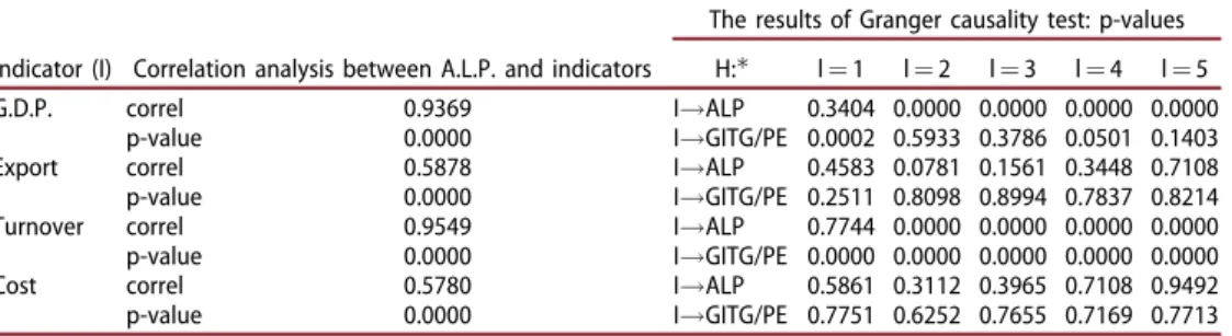
Since exogenous variables will also be included into model (3), the correlation and causality analyses are made upon these variables as well. Although Spearman’s correl-ation coefficient shows a comparatively strong correlcorrel-ation between A.L.P. and all exogenous variables, Granger causality test indicates that only G.D.P. and turnover Granger-cause A.L.P. (seeTable 5). G.I.T.G. per P.E. is also caused by these two vari-ables. As export and cost do not have any impact on A.L.P., they will not be included
Table 2. The difference between the real A.L.P. and its forecast.
Country Real ALP in 2015 Difference Country Real ALP in 2015 Difference
Bulgaria 11.40 15.4% Italy 58.84 8.1% Romania 12.76 16.7% France 71.70 5.9% Latvia 17.36 9.0% Germany 73.55 7.3% Lithuania 19.06 10.3% Finland 74.03 22.9% Croatia 19.22 18.3% Luxembourg 78.06 18.0% Estonia 24.59 17.8% Austria 82.62 6.1% Poland 24.83 20.5% U.K. 88.96 17.5% Slovakia 27.25 3.7% Denmark 89.32 9.5%
Czech Republic 28.31 2.3% Sweden 90.07 12.7%
Portugal 28.69 16.3% Netherlands 93.10 2.8% Hungary 30.56 8.4% Norway 96.62 11.0% Cyprus 31.40 28.4% Belgium 103.51 3.6% Greece 35.28 30.9% Switzerland 150.86 38.5% Slovenia 37.33 1.8% Ireland 441.73 207.5% Spain 57.62 12.5%
into the model as exogenous variables in order to minimise the number of the inde-pendent variables and maximise the degree of freedom.
The unit root test shows that all the indicators under research are stationary (see Table 6). A.L.P., G.I.M.E. per P.E. and G.D.P. are stationary when an intercept and a trend are included (in both of the following cases: a common unit root process and an individual unit root process), while all other indicators are stationary when an intercept is included (in both of the following cases: a common unit root process and an individ-ual unit root process). The stationary processes let avoid the spurious regression.
4.3. Vector autoregression
Granger causality test reveals the reciprocal relation between A.L.P. and G.I.T.G. per P.E. Thus, the relation between these indicators is found to be determined by V.A.R. with two endogenous variables (A.L.P. and G.I.T.G. per P.E.) and two exogenous var-iables (G.D.P. and turnover). The equations are solved by employing the ordinary least squares estimation.
Table 3. The results of the correlation analysis.
Indicator G.I.T.G./P.E. G.I.L./P.E. G.I.E.B.S./P.E. G.I.C.B./P.E. G.I.M.E./P.E. N.I.T.G./P.E.
Correlation 0.8815 0.2337 0.4675 0.3321 0.8326 0.7961
p-value 0.0000 0.0009 0.0000 0.0000 0.0000 0.0000
Table 4. The results of Granger causality test: p-values.
Indicator (I) H: l¼1 l¼2 l¼3 l¼4 l¼5 G.I.T.G./P.E. I!ALP 0.4861 0.0000 0.0000 0.0000 0.0000 ALP!I 0.0000 0.0000 0.0000 0.0000 0.0000 G.I.L./P.E. I!ALP 0.4631 0.1474 0.7686 0.1466 0.0141 ALP!I 0.0327 0.4530 0.1097 0.1736 0.1299 G.I.E.B.S./P.E. I!ALP 0.0005 0.0030 0.0000 0.0000 0.0000 ALP!I 0.1756 0.0225 0.0015 0.0338 0.0012 G.I.C.B./P.E. I!ALP 0.6302 0.5431 0.9581 0.0431 0.0702 ALP!I 0.0222 0.0204 0.0251 0.6063 0.1068 G.I.M.E./P.E. I!ALP 0.0236 0.0755 0.0389 0.4535 0.0091 ALP!I 0.1598 0.1916 0.3143 0.2229 0.0606 N.I.T.G./P.E. I!ALP 0.0000 0.1818 0.1130 0.7654 0.0172 ALP!I 0.0000 0.2050 0.0277 0.0201 0.2787
Note:the hypothesis that I does not Granger-cause A.L.P. (I!ALP) is tested in the first row, while the hypothesis that A.L.P. does not Granger-cause I (A.L.P.!I) is tested in the second row.
Table 5. The results of the correlation and causality analyses upon exogenous variables. Indicator (I) Correlation analysis between A.L.P. and indicators
The results of Granger causality test: p-values H: l¼1 l¼2 l¼3 l¼4 l¼5
G.D.P. correl 0.9369 I!ALP 0.3404 0.0000 0.0000 0.0000 0.0000
p-value 0.0000 I!GITG/PE 0.0002 0.5933 0.3786 0.0501 0.1403
Export correl 0.5878 I!ALP 0.4583 0.0781 0.1561 0.3448 0.7108
p-value 0.0000 I!GITG/PE 0.2511 0.8098 0.8994 0.7837 0.8214
Turnover correl 0.9549 I!ALP 0.7744 0.0000 0.0000 0.0000 0.0000
p-value 0.0000 I!GITG/PE 0.0000 0.0000 0.0000 0.0000 0.0000
Cost correl 0.5780 I!ALP 0.5861 0.3112 0.3965 0.7108 0.9492
p-value 0.0000 I!GITG/PE 0.7751 0.6252 0.7655 0.7169 0.7713
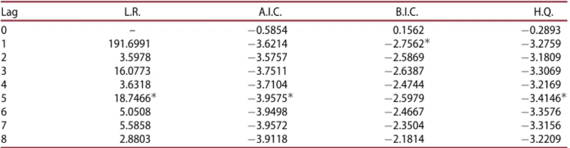
The sequential modified L.R. test statistic, the A.I.C., B.I.C., and the H.Q. are used for lag length selection. Most of the criteria advises the lag of 5 as the most appropri-ate, except B.I.C. which gets its minimum value when lag is 1 (seeTable 7).
The V.A.R. model is estimated starting with five lags of endogenous and exogen-ous variables. The results of such model are provided in Table 8. The models with smaller number of lags are also developed, but as none of them improves the charac-teristics of the model, their results are not provided in this article.
The estimated V.A.R. residual Portmanteau tests of autocorrelations and correlograms indicate that the residuals do not show any autocorrelation. However, the normality of the residuals is rejected (joint Jargue-Bera¼ 168.55 and p-value ¼0.0000), and the het-eroscedasticity test is not satisfactory (joint test Chi-sq.¼260.99, p-value¼0.0000).
Summarising, the V.A.R. confirms a positive impact of investment in tangibles on productivity, but this impact is not strong. Thus, it is useful to test if this effect varies among the countries. Moreover, the V.A.R. model has a limitation that endogenous vari-ables of periodt cannot be included into the model (only lag values are evaluated). As correlation analysis indicates that G.I.T.G. per P.E (endogenous variable) has strong sig-nificant simultaneous relationship with A.L.P. its value of the current period should also be evaluated. Therefore, the testing is performed by employing panel regression analysis.
4.4. Panel regression analysis
As A.L.P. is caused by the delayed effect of investment per P.E., equation (3) is expanded by its lag values. The previous analysis revealed that A.L.P. is a strongly autoregressive process, which, in its turn, proposes that the lag values of the depend-ent variable can increase the precision of the model. A time trend is also included in panel regressions as a proxy for multifactor productivity. In this way, the following model is developed: ln Yt Lt ¼b0þb1tþb2ln Yt1 Lt1 þ:::þb6ln Yt5 Lt5 þb7ln Kt Lt þb8ln Kt1 Lt1 þ:::þb12ln Kt5 Lt5 þb13ln GDPð tÞ þb14ln GDPð t1Þ þ:::þb18ln GDPð t5Þ þb19ln Turnoverð tÞ þb20ln Turnoverð t1Þ þ:::þb24ln Turnoverð t5Þ (5)
Table 6. Probabilities of unit root test (H0: process has a unit root). Indicator
Assumes common unit root process (Levin, Lin & Chu) Assumes individual unit root process (A.D.F.)
None With intercept
With trend
and intercept None With intercept
With trend and intercept A.L.P. 1.0000 0.1362 0.0000 1.0000 0.9993 0.0005 G.I.T.G./P.E. 0.9139 0.0000 0.0000 0.9935 0.0028 0.0003 G.I.L./P.E. 1.0000 0.0000 0.0000 0.7714 0.0006 0.0001 G.I.E.B.S./P.E. 0.0155 0.0000 0.0000 0.2171 0.0004 0.0036 G.I.C.B./P.E. 0.7329 0.0000 0.0000 0.8918 0.0051 0.0003 G.I.M.E./P.E. 0.3871 0.0168 0.0000 0.9557 0.6294 0.0273 N.I.T.G./P.E. 0.9866 0.0000 0.0000 0.9956 0.0399 0.0017 G.D.P. 1.0000 0.0000 0.0000 1.0000 0.2300 0.0000 Turnover 1.0000 0.0000 0.0000 1.0000 0.0023 0.0179
herebi are the parameters of the panel regression model. The parameters of model (5) are estimated by employing the panel least squares method.
Firstly, the impact of G.I.T.G. per P.E. (Kt
Lt ¼ ðGITG=PEÞt) on A.L.P. (
Yt
Lt ¼ALPtÞ
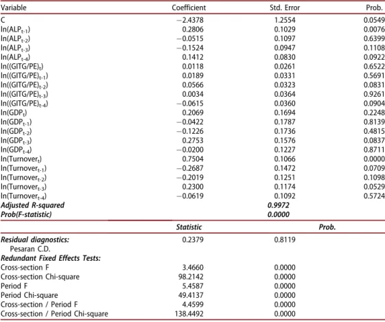
is analysed. After the parameters of model (5) have been estimated, the redundant variable test is performed. It shows that all five period lagged variables and the trend component are redundant. This test reveals that some other variables are also redun-dant, but they are not eliminated as this can cause the correlation in the residuals. The purpose is to find the model with the smallest number of the variables with no cross-section dependence in the residuals. Since tis relatively small, the focus falls on the results of the asymptotically standard normal Pesaran C.D. test. The results of such model with time and cross-section fixed effects are presented inTable 9.
The precision of the model is very high (adjusted R2is 0.9972), and the model is sig-nificant, although most of the independent variables are not significant at the significance level of 0.05. Pesaran C.D. test indicates that there is no cross-section dependence in the
Table 7. V.A.R. lag order selection criteria.
Lag L.R. A.I.C. B.I.C. H.Q.
0 – 0.5854 0.1562 0.2893 1 191.6991 3.6214 2.7562 3.2759 2 3.5978 3.5757 2.5869 3.1809 3 16.0773 3.7511 2.6387 3.3069 4 3.6318 3.7104 2.4744 3.2169 5 18.7466 3.9575 2.5979 3.4146 6 5.0508 3.9498 2.4667 3.3576 7 5.5858 3.9572 2.3504 3.3156 8 2.8803 3.9118 2.1814 3.2209
Table 8. The results of the V.A.R. model. Variable
ln(ALPt) ln((GITG/PE)t)
Coefficient Std. Error t-statistics Coefficient Std. Error t-statistics
C 0.0732 0.1772 0.4129 0.8157 0.6327 1.2892 ln(ALPt-1) 0.8051 0.1102 7.3056 1.1887 0.3935 3.0212 ln(ALPt-2) 0.2382 0.1324 1.7984 3.2291 0.4728 6.8295 ln(ALPt-3) 0.2076 0.1240 1.6733 1.4988 0.4429 3.3845 ln(ALPt-4) 0.1077 0.1108 0.9721 0.0746 0.3956 0.1887 ln(ALPt-5) 0.0158 0.0926 0.1708 0.6097 0.3306 1.8443 ln((GITG/PE)t-1) 0.0763 0.0385 1.9845 0.4600 0.1373 3.3499 ln((GITG/PE)t-2) 0.0112 0.0450 0.2490 0.1900 0.1608 1.1817 ln((GITG/PE)t-3) 0.0335 0.0452 0.7410 0.0468 0.1612 0.2902 ln((GITG/PE)t-4) 0.0133 0.0518 0.2563 0.4071 0.1849 2.2015 ln((GITG/PE)t-5) 0.0605 0.0430 1.4086 0.4265 0.1534 2.7804 ln(GDPt) 0.3952 0.2077 1.9034 3.2284 0.7414 4.3545 ln(GDPt-1) 0.4499 0.3023 1.4885 3.0825 1.0791 2.8564 ln(GDPt-2) 0.1184 0.2254 0.5251 1.3632 0.8048 1.6938 ln(GDPt-3) 0.0831 0.2275 0.3655 0.9274 0.8122 1.1419 ln(GDPt-4) 0.2475 0.2121 1.1670 0.9034 0.7571 1.1933 ln(GDPt-5) 0.1112 0.1317 0.8443 0.6356 0.4701 1.3521 ln(Turnovert) 0.6192 0.1146 5.4039 0.0855 0.4091 0.2091 ln(Turnovert-1) 0.6765 0.1876 3.6066 0.0767 0.6697 0.1146 ln(Turnovert-2) 0.1201 0.1706 0.7040 1.3598 0.6091 2.2323 ln(Turnovert-3) 0.2437 0.1455 1.6755 1.0918 0.5193 2.1025 ln(Turnovert-4) 0.0116 0.1290 0.0901 0.3829 0.4607 0.8310 ln(Turnovert-5) 0.0202 0.0939 0.2147 0.2888 0.3353 0.8615 Adjusted R-squared 0.9951 0.8826 Determinant resid covariance 8.17E-05
residuals. The probabilities of ‘F’ and ‘Chi-square’ statistics strongly reject the null hypothesis proposing that time and cross-section effects are redundant.
Labour productivity persistence can be captured by the sum of the autoregressive coefficients. The sum of the autoregressive coefficients remains positive and equal to 0.2179 (standard error is 0.1194). The long-run multiplier is given by the sum of the contemporaneous and lag investment coefficient estimates (it equals to 0.0292 and standard error is 0.0531) divided by 1 minus the sum of the productivity coefficient estimates (autoregressive parameters), given that the key stability condition holds. Thus, the long-run effect of G.I.T.G. per P.E. on A.L.P. amounts to 0.0373 with a standard error of 0.0667. This means that a 1% increase in G.I.T.G. per P.E. has a 0.0373% long-run effect on A.L.P. The Wald test accepts the null hypothesis about its equality to zero (prob(t-statistic) ¼ 0.5766; prob(F-statistic) ¼ 0.5766; prob(chi-square)¼0.5754). This shows that the effect is not significant.
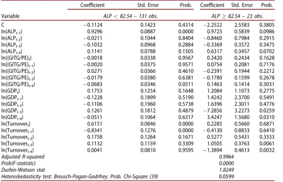
The multiple threshold test (Bai-Perron tests of Lþ1 vs. L sequentially determined thresholds) determines four A.L.P. thresholds which are significant at the 0.05 level. Table 10 presents the results of the threshold regression with one threshold. In the case of more thresholds, the coefficient of one period lagged A.L.P. is higher than 1, thus the stability condition is not satisfied.
The sum of the productivity coefficient estimates (contemporaneous and lag) is negative and equals to 0.0630 when A.L.P.<82.54, meanwhile in the case of
Table 9. The results of the panel regression analysis considering the impact of G.I.T.G./P.E.
Variable Coefficient Std. Error Prob.
C 2.4378 1.2554 0.0549 ln(ALPt-1) 0.2806 0.1029 0.0076 ln(ALPt-2) 0.0515 0.1097 0.6399 ln(ALPt-3) 0.1524 0.0947 0.1108 ln(ALPt-4) 0.1412 0.0830 0.0922 ln((GITG/PE)t) 0.0118 0.0261 0.6522 ln((GITG/PE)t-1) 0.0189 0.0331 0.5691 ln((GITG/PE)t-2) 0.0566 0.0323 0.0831 ln((GITG/PE)t-3) 0.0034 0.0364 0.9261 ln((GITG/PE)t-4) 0.0615 0.0360 0.0904 ln(GDPt) 0.2069 0.1694 0.2248 ln(GDPt-1) 0.0422 0.1787 0.8139 ln(GDPt-2) 0.1226 0.1736 0.4815 ln(GDPt-3) 0.2753 0.1576 0.0837 ln(GDPt-4) 0.0200 0.1227 0.8711 ln(Turnovert) 0.7504 0.1066 0.0000 ln(Turnovert-1) 0.2687 0.1472 0.0709 ln(Turnovert-2) 0.2019 0.1251 0.1098 ln(Turnovert-3) 0.2300 0.1174 0.0529 ln(Turnovert-4) 0.0619 0.1092 0.5724 Adjusted R-squared 0.9972 Prob(F-statistic) 0.0000 Statistic Prob. Residual diagnostics: Pesaran C.D. 0.2379 0.8119
Redundant Fixed Effects Tests:
Cross-section F 3.4660 0.0000
Cross-section Chi-square 98.2142 0.0000
Period F 5.4587 0.0000
Period Chi-square 49.4137 0.0000
Cross-section / Period F 4.4599 0.0000
higher A.L.P., the sum of the coefficient estimates is positive and equals to 0.1465. The long-run multiplier is 0.7808 when A.L.P.<82.54, and 0.2531 when A.L.P.82.54. Thus, a 1% increase in G.I.T.G. per P.E. has a 0.2531% long-run effect on A.L.P. in the countries with high productivity, such as Switzerland (since 2009), Norway (since 2007, except 2009), the U.K. (since 2015), Sweden (since 2013), Austria (since 2015), the Netherlands (since 2010), Ireland (since 2005), Denmark (since 2010, except 2011–2012), Luxembourg (only in 2007–2008) and Belgium (since 2006, except 2009). At the same time, the negative effect of invest-ment in tangible goods on productivity is observed in all other European coun-tries, i.e., it is found that a 1% increase in G.I.T.G. per P.E. has a 0.7808% long-run effect on A.L.P.
G.I.T.G. consists of four components: G.I.L., G.I.E.B.S., G.I.C.B., and G.I.M.E.. Therefore, it is useful to find out how A.L.P. depends on these components. The Granger causality test shows that only G.I.E.B.S. per P.E. and G.I.M.E. per P.E. cause A.L.P. That is why equations (3) and (5) will be estimated including the two types of investment.
Model (5) parameters, which consist of four independent variables (G.I.E.B.S./P.E., G.I.M.E./P.E., G.D.P. and turnover) and their lags, are estimated by panel least squares. Then, the redundant variable test is performed in order to reduce the num-ber of the independent variables and increase the degree of freedom. It shows that from three to five period lagged variables and trend component are redundant. The purpose is to find the model with the smallest number of variables with no cross-sec-tion dependence (correlacross-sec-tion) in the residuals. The results of such model with the time and cross-section fixed effects are presented inTable 11.
Table 10. The results of the threshold regression. Variable
Coefficient Std. Error Prob. Coefficient Std. Error Prob.
ALP<82.54–131 obs. ALP82.54–23 obs.
C 0.1124 0.1423 0.4314 2.2522 2.5583 0.3805 ln(ALPt-1) 0.9296 0.0887 0.0000 0.9723 0.5839 0.0986 ln(ALPt-2) 0.0211 0.1044 0.8404 0.8460 0.7984 0.2915 ln(ALPt-3) 0.1032 0.0968 0.2884 0.3369 0.3572 0.3475 ln(ALPt-4) 0.1141 0.0788 0.1505 0.6317 0.3457 0.0702 ln((GITG/PE)t) 0.0018 0.0338 0.9567 0.3420 0.2434 0.1628 ln((GITG/PE)t-1) 0.0020 0.0375 0.9571 0.0754 0.2081 0.7176 ln((GITG/PE)t-2) 0.0271 0.0366 0.4610 0.2391 0.1944 0.2212 ln((GITG/PE)t-3) 0.0179 0.0380 0.6381 0.1780 0.1599 0.2678 ln((GITG/PE)t-4) 0.0683 0.0346 0.0511 0.1463 0.1414 0.3031 ln(GDPt) 0.1753 0.1254 0.1648 1.2084 1.1073 0.2775 ln(GDPt-1) 0.1228 0.1899 0.5190 1.4242 2.3700 0.5491 ln(GDPt-2) 0.1106 0.1960 0.5738 1.6396 2.3011 0.4776 ln(GDPt-3) 0.1261 0.1812 0.4879 7.2856 3.2273 0.0259 ln(GDPt-4) 0.0511 0.1064 0.6317 3.4247 1.5680 0.0310 ln(Turnovert) 0.6151 0.0846 0.0000 0.2285 0.5660 0.6871 ln(Turnovert-1) 0.8341 0.1276 0.0000 0.4130 0.8833 0.6410 ln(Turnovert-2) 0.1758 0.1264 0.1671 0.5277 0.5431 0.3333 ln(Turnovert-3) 0.1132 0.1159 0.3309 1.0505 0.3763 0.0061 ln(Turnovert-4) 0.0041 0.0810 0.9595 1.3894 0.4613 0.0032 Adjusted R-squared 0.9964 Prob(F-statistic) 0.0000 Durbin-Watson stat 1.8249 Heteroskedasticity test: Breusch-Pagan-Godrfrey: Prob. Chi-Square (39) 0.0599
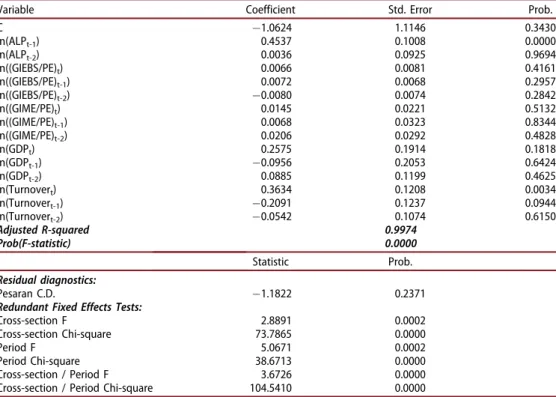
The precision of the model is very high (adjusted R2 is 0.9974) and the model is significant, although most of the independent variables are not significant at the sig-nificance level of 0.05. Pesaran C.D. test indicates that there exists no cross-section dependence in the residuals. The redundant fixed effects test rejects the null hypoth-esis that the time and cross-section effects are redundant.
The sum of the autoregressive coefficients of A.L.P. remains positive and equal to 0.4573 (standard error is 0.1238). The sum of the contemporaneous and lag G.I.E.B.S. per P.E. coefficient equals to 0.0058 (standard error is 0.0129), and the sum of the con-temporaneous and lag G.I.M.E. per P.E. coefficient equals to 0.0419 (standard error is 0.0489). The long-run effect of G.I.E.B.S. per P.E. on A.L.P. amounts to 0.0106 with a standard error of 0.0242. Thus, a 1% increase in G.I.E.B.S. per P.E. has a 0.0106% long-run effect on A.L.P. The Wald test accepts the null hypothesis about its equality to zero (prob(t-statistic) ¼ 0.6618; prob(F-statistic) ¼ 0.6618; prob(chi-square) ¼ 0.6608). The long-run effect of G.I.M.E. per P.E. on A.L.P. amounts to 0.0771 with a standard error of 0.0872. This means that a 1% increase in G.I.M.E. per P.E. has a 0.0771% long-run effect on A.L.P. The Wald test accepts the null hypothesis about its equality to zero (prob(t-statistic)¼0.3787; prob(F-statistic)¼0.3787; prob(chi-square)¼0.3765).
The multiple threshold test (Bai-Perron tests of Lþ1 vs. L sequentially determined thresholds) determines one A.L.P. threshold which is significant at the 0.05 level, but the coefficient of one period lagged A.L.P. is higher than 1, which means that the stability condition is not satisfied. For this reason, the results of the multiple threshold regression are not presented in the article.
Table 11. The results of the panel regression analysis with consideration of the impact of G.I.E.B.S./P.E. and G.I.M.E./P.E.
Variable Coefficient Std. Error Prob.
C 1.0624 1.1146 0.3430 ln(ALPt-1) 0.4537 0.1008 0.0000 ln(ALPt-2) 0.0036 0.0925 0.9694 ln((GIEBS/PE)t) 0.0066 0.0081 0.4161 ln((GIEBS/PE)t-1) 0.0072 0.0068 0.2957 ln((GIEBS/PE)t-2) 0.0080 0.0074 0.2842 ln((GIME/PE)t) 0.0145 0.0221 0.5132 ln((GIME/PE)t-1) 0.0068 0.0323 0.8344 ln((GIME/PE)t-2) 0.0206 0.0292 0.4828 ln(GDPt) 0.2575 0.1914 0.1818 ln(GDPt-1) 0.0956 0.2053 0.6424 ln(GDPt-2) 0.0885 0.1199 0.4625 ln(Turnovert) 0.3634 0.1208 0.0034 ln(Turnovert-1) 0.2091 0.1237 0.0944 ln(Turnovert-2) 0.0542 0.1074 0.6150 Adjusted R-squared 0.9974 Prob(F-statistic) 0.0000 Statistic Prob. Residual diagnostics: Pesaran C.D. 1.1822 0.2371
Redundant Fixed Effects Tests:
Cross-section F 2.8891 0.0002
Cross-section Chi-square 73.7865 0.0000
Period F 5.0671 0.0002
Period Chi-square 38.6713 0.0000
Cross-section / Period F 3.6726 0.0000
Considering the results, it is clear that the impact of investment in asset per P.E. on A.L.P. in European manufacturing industry differs among the countries. For this reason, the analysis of the correlation between A.L.P. and various types of investment per P.E. for each of the countries is performed. The results are presented inTable 12.
The results indicate that A.L.P. significantly (at a significance level of 0.1 at least) correlates with all of the types of investment only in the Netherlands. Nevertheless, A.L.P. has a high or moderate correlation with most types of investment in the U.K., Switzerland, Sweden and Belgium which are characterised by high A.L.P. (lower than median values of A.L.P. in 2015 are marked in red in Table 12). However, three countries, i.e., Croatia, Hungary and Cyprus, where A.L.P. is low, also have a positive and significant correlation between productivity and many types of investment. It means that a significant increase in investment in asset per P.E. (especially investment in machinery and equipment per P.E.) in these countries lets improve the A.L.P. An increase in G.I.M.E. per P.E. also improves the A.L.P. in Estonia, Poland, the Czech Republic, Slovakia and Lithuania. Meanwhile, the A.L.P. in Greece and Portugal cor-relates mostly with G.I.C.B., while the correlation with G.I.E.B.S. per P.E. as well as G.I.M.E. per P.E. is negative. The most problematic countries are Romania and Latvia where the coefficients of the correlation between A.L.P. and all of the types of invest-ment per P.E. are low and many of them are even negative. A low or even negative correlation between productivity and various types of investment is observed even in
Table 12. The coefficients of the correlation between A.L.P. and various types of investment per P.E.
Country G.I.T.G./P.E. G.I.L./P.E. G.I.E.B.S./P.E. G.I.C.B./P.E. G.I.M.E./P.E. N.I.T.G./P.E. A.L.P. U.K. 0.92 0.75 0.54 0.91 0.96 0.94 88.96 Switzerland 0.83 0.72 0.74 1.00 0.90 0.71 150.86 Sweden 0.82 – – 0.73 0.77 0.82 90.07 Croatia 0.81 0.13 0.70 0.40 0.94 0.83 19.22 Hungary 0.81 0.15 0.16 0.68 0.90 0.81 30.56 Cyprus 0.80 0.73 0.49 0.81 0.90 0.88 31.40 Belgium 0.78 0.43 0.79 0.37 0.67 0.72 103.51 Netherlands 0.76 0.66 0.64 0.70 0.59 0.65 93.10 Germany 0.71 0.46 0.12 0.53 0.64 0.58 73.55 Estonia 0.70 0.48 0.37 0.28 0.86 0.89 24.59 Luxembourg 0.68 0.14 0.42 0.02 0.71 0.75 78.06 Poland 0.67 0.78 0.13 0.46 0.72 0.63 24.83 France 0.64 – – – – 0.69 71.70 Ireland 0.61 0.41 0.59 0.04 0.79 0.66 441.73 Czech Republic 0.59 0.18 0.32 0.08 0.68 0.59 28.31 Finland 0.59 0.83 0.15 0.11 0.40 0.30 74.03 Greece 0.54 0.26 0.21 0.75 0.06 0.46 35.28 Austria 0.53 0.02 0.52 0.44 0.62 0.41 82.62 Bulgaria 0.47 0.14 0.40 0.01 0.46 0.39 11.40 Romania 0.35 0.48 – 0.05 0.18 0.20 12.76 Spain 0.29 0.01 0.67 0.49 0.41 0.28 57.62 Portugal 0.20 0.18 0.63 0.79 0.10 0.26 28.69 Slovenia 0.07 0.15 0.54 0.13 0.59 0.42 37.33 Slovakia 0.07 0.36 0.51 0.60 0.62 0.70 27.25 Norway 0.02 0.94 – 0.04 0.13 0.01 96.62 Denmark 0.05 0.12 0.36 0.11 0.23 0.21 89.32 Lithuania 0.08 0.23 0.36 0.23 0.65 0.27 19.06 Latvia 0.11 0.33 0.08 0.57 0.11 0.14 17.36 Italy 0.19 0.34 0.17 0.69 0.23 0.39 58.84 Note:p<0.1,p<0.05,p<0.01.
a few more countries with higher than median A.L.P. These countries are Italy and Denmark. Since A.L.P. in Romania, Latvia, Italy and Denmark is growing, it means that it is affected by some other factors rather than investment in tangible assets, and the latter investment is used inefficiently.
5. Conclusion
Researchers have been investigating the effects of tangible assets on the growth of labour productivity for more than five decades. The relation between these indicators is commonly described by the Solow model, which states that the changes in labour productivity occur due to technical change and the changes in the capital–labour ratio. It means that the growth of capital causes an increase in labour productivity.
This research conditionally confirms a positive relation between A.L.P. and invest-ment in tangible assets divided by persons for the European manufacturing industry. The Granger causality test reveals the reciprocal causality between A.L.P. and G.I.T.G. per P.E. as well as G.I.E.B.S. per P.E. The causality is also found between A.L.P. and other types of investment when a certain lag length is set, but this evidence is not strong.
The V.A.R. model indicate that G.I.T.G. per P.E. has a positive impact on A.L.P. for five years, although this effect is not strong. The panel regression analysis shows that the differences in the relationship between productivity and investment exist among the countries, i.e., the significant cross-section as well as time fixed effects could be observed. If all European countries are considered, a 1% increase in G.I.T.G. per P.E. has a 0.0373% long-run effect on A.L.P. Considering various types of investment, a 1% increase in G.I.E.B.S. per P.E. has only a 0.0106% long-run effect on A.L.P. Meanwhile, a 1% increase in G.I.M.E. per P.E. has a 0.0771% long-run effect on A.L.P.
The multiple threshold test, however, distinguishes a significant threshold of A.L.P. at the level of e82.54,000 and reveals that a positive effect of investment in tangibles on productivity could be observed only in several countries. A 1% increase in G.I.T.G. per P.E. has a 0.2531% long-run effect on A.L.P. in the countries with high productivity, such as Switzerland, Norway, the U.K., Sweden, Austria, the Netherlands, Ireland, Denmark, and Belgium. Meanwhile, a negative effect of invest-ment in tangible goods on productivity is observed in all other European countries, i.e., a 1% increase in G.I.T.G. per P.E. has a -0.7808% long-run effect on A.L.P.
The analysis of the correlation between A.L.P. and various types of investment per P.E. for each country shows that A.L.P. significantly correlates with all of the types of investment only in the Netherlands. A.L.P. could be improved by increasing most types of investment in the U.K., Switzerland, Sweden and Belgium, which are characterised by high A.L.P., as well as in three other countries where productivity is low, i.e., Croatia, Hungary, and Cyprus. An increase in investment in machinery and equipment per P.E. also improves A.L.P. in Estonia, Poland, the Czech Republic, Slovakia and Lithuania. Meanwhile, A.L.P. in Greece and Portugal correlates mostly with G.I.C.B., while the cor-relation with G.I.E.B.S. per P.E. and G.I.M.E. per P.E. is negative.
The research reveals that many European countries use investment inefficiently. The most problematic countries in this regard are Romania and Latvia where the
coefficients of the correlation between A.L.P. and all of the types of investment per P.E. are low and many of them are even negative. A low or even negative correlation between productivity and various types of investment is observed even in Italy and Denmark where A.L.P. is higher than median. Since A.L.P. in these countries is grow-ing, it means that the growth is affected by other factors rather than investment in tangible assets, and investment in tangible assets is used inefficiently.
References
Acemoglu, D. (2008). Introduction to Modern economic growth. Princeton, NJ: Princeton University Press. ISBN 9781400835775.
Arrow, K. J. (1962). The economic implications of learning by doing. The Review of Economic Studies,29(3), 155–173. doi:10.2307/2295952
Baily, M. N. (1981). The Productivity Growth Slowdown and Capital Accumulation. The American Economic Review,71(2), 326–331.
Bini, M., Nascia, L., & Zeli, A. (2014). Industry profiles and economic performances: A firm-data-based study for Italian industries. Statistica Applicata – Italian Journal of Applied Statistics,23(3), 331–345.
Black, S., & Lynch, L. (2001). How to compete: The impact of workplace practices and infor-mation technology on productivity.Review of Economics and Statistics, 83(3), 434–445. doi: 10.1162/00346530152480081
Cette, G., Fernald, J., & Mojon, B. (2016). The pre-Great Recession slowdown in productivity. European Economic Review,88, 3–20. doi:10.1016/j.euroecorev.2016.03.012.
Chaudhuri, A., Koudal, P., & Seshadri, S. (2010). Productivity and capital investments: An empirical study of three manufacturing industries in India. IIMB Management Review, 22(3), 65–79. doi:10.1016/j.iimb.2010.04.012.
Chen, K., Gong, X., & Marcus, R. D. (2014). The New Evidence to Tendency of Convergence in Solow model.Economic Modelling,41, 263–266.
Ding, S., & Knight, J. (2009). Can the augmented Solow model explain China’s remarkable economic growth? A cross-country panel data analysis.Journal of Comparative Economics, 37(3), 432–452. doi:10.1016/j.jce.2009.04.006
Fare, R., Grosskopf, S., & Margaritis, D. (2006). Productivity growth and convergence in the European Union.Journal of Productivity Analysis,25(1-2), 111–141. doi: 10.1007/s11123-006-7134-x
Grifell-Tatje, E. & Lovell, C. A. K. (2015). Productivity Accounting: the Economics of Business Performance. New York, United States: Cambridge University Press. doi:10.1017/ CBO9781139021418.
Lucas, R. E. Jr.(1988). On the mechanics of economic development. Journal of Monetary Economics,22(1), 3–42. doi:10.1016/0304-3932(88)90168-7
Mankiw, G. N., Romer, D., & Weil, D. N. (1992). A contribution to the empirics of economic growth.The Quarterly Journal of Economics,107(2), 407–437. doi:10.2307/2118477
Mankiw, G. N., & Taylor, M. P. (2008).Macroeconomics. New York: Worth Publishers. Nilsen, O. A., Raknerud, A., Rybalka, M., & Skjerpen, T. (2008). Lumpy investments, factor
adjustments, and labour productivity.Oxford Economic Papers,61(1), 104–127. doi:10.1093/ oep/gpn026
Rebelo, S. (1991). Long-run policy analysis and long-run growth.Journal of Political Economy, 99(3), 500–521. doi:10.1086/261764
Romer, P. M. (1990). Endogenous technological change. Journal of Political Economy, 98(5, Part 2), S71–S101. doi:10.1086/261725
Salinas-Jimenez, M., Alvarez-Ayuso, I., & Delgado-Rodriguez, J. (2006). Capital accumulation and TFP growth in the EU: A production frontier approach.Journal of Policy Modeling,28, 195–205. doi:10.1016/j.jpolmod.2005.07.008
Shaw, K. (2004). The human resources revolution: is it a productivity driver? In A B. Jaffe, J Lerner and S Stern (Eds.). NBER book innovation policy and the economy (Vol. 4, pp. 69–114). Cambridge: The MIT Press. doi:10.1086/ipe.4.25056162
Solow, R. (1956). A contribution to the theory of economic growth. Quarterly Journal of Economics,70(1), 56–94.
Stiroh, K. J. ( (2000). ). Investment and productivity growth: A survey from the neoclassical and new growth perspectives. Industry Canada Research Publications Program. Occasional Paper Number 24.
Strobel, T. (2011). The economic impact of capital-skill complementarities on sectoral product-ivity growth- new evidence from industrialized industries during the new economy. 17th International Panel Data Conference[Montreal. July 2011].
Swierczynska, K. (2017). Structural transformation and economic development in the best per-forming sub-Saharan African states. Equilibrium.Equilibrium, 12(4), 547–571. doi:10.24136/ eq.v12i4.29