BEEF CATTLE PRODUCTION PRACTICES: WHAT ARE THEY WORTH?
A Dissertation by
MYRIAH DAWN JOHNSON
Submitted to the Office of Graduate and Professional Studies of Texas A&M University
in partial fulfillment of the requirements for the degree of DOCTOR OF PHILOSOPHY
Chair of Committee, Jason E. Sawyer Co-Chair of Committee, James W. Richardson Committee Members, Tryon A. Wickersham
David P. Anderson Head of Department, H. Russell Cross
May 2016
Major Subject: Animal Science
ii ABSTRACT
Multiple investigations were undertaken to evaluate the value of three facets of beef cattle production. In the first study, price and quantity effects of β-adrenergic agonists removal from beef cattle production were estimated using a stochastic equilibrium displacement model. In the long run, beef consumers, packer/processors, and feedlots face reduced prices and increased quantities. Price and quantity of feeder calves increases. Even with reduced prices for consumers, there are also reduced prices for other market sectors, making them less profitable and threatening their economic sustainability. It also increases the number of animals needed to meet demand and increases the demand on environmental resources. β-adrenergic agonists improve both environmental and economic sustainability.
In the second study, fatty acid composition and shear force analysis, along with a discrete choice experiment were conducted to evaluate consumer preferences for sirloin steaks from steers fed post-extraction algal residue (PEAR) or conventional (grain-based) feeding systems, tenderness, quality grade, origin, use of growth technologies, and price of beef. Ninety six consumers participated in a sensory tasting panel before completing a choice set survey; 127 consumers completed only the choice set survey. Sensory tasting of the products was observed to alter the preferences of consumers. Consumers completing only the survey perceived beef from PEAR-fed cattle negatively compared to beef from grainfed cattle, with a willingness to pay (WTP) discount of -$1.17/kg. With sensory tasting the WTP for beef from PEAR-fed cattle was not
iii
discounted relative to beef from grain-fed cattle (P = 0.21). No tasting consumers had much higher stated WTP values for credence attributes. Factors that influence the eating experience (tenderness, quality grade) dominated as the most influential attributes on WTP among the tasting group.
In the final study, variables influencing the mortality of feedlot cattle during their last 48 days on feed (DOF) were determined. A predictive model of mortality in the feedlot for the upcoming week was also built. Ordinary least squares, Poisson, and Negative Binomial regressions were estimated. Factors identified as influencing mortality in cattle during their last 48 DOF include weight, time of year placed in the feedyard, weather, number of animals not receiving β-AAs, feeder cattle price, DOF, and previous mortality within the population, along with combinations of several of these factors.
Results from these studies suggest there is value in each practice evaluated. Ultimately, each practice can improve economic and/or environmental sustainability. Production elements must be carefully evaluated from many angles before decisions on whether to implement or remove the practices can be decided.
iv
DEDICATION
Jeremiah 29:11
“For I know the plans I have for you…”
This doctoral work is dedicated to God. His plans are far better than my own. When I began I thought I knew the plan, but I didn’t. God used this as a way to draw me closer to Him, allowing me to grow spiritually. He revealed to me a path for my education and career that was far better than one I could have ever imagined, allowing me to pursue my
v
ACKNOWLEDGEMENTS
Chris, we first started dating when I began this Ph.D. I don’t know how or why you decided to remain with me through the turbulence of the first year when you hardly knew me. God placed you in my life at exactly the right time though. He knew I needed your love, support, and encouragement. After the first year I knew that if we had made it through that, then we would be together for a very long time. Today I am thankful to be your wife and that you are my husband. Your love does not fail even when I am relentlessly stubborn, tired, and cranky. I am excited to see what lies ahead of us. No matter the ups and downs I want to be right by your side. I love you so much.
Mom, Dad, & Dakota, my original support team. I would have never made it down this path if you had not helped me get the best start so many years ago. You have given me a lifetime of love and support. Thank you for being there for EVERYTHING, whether it was my first steps, dance recital, cross-country meets, band performances, the bad days and the good days, and never giving up on me. When I wanted to quit you didn’t allow it. You pushed me to be more than I thought I could, telling me that my education is the one thing that can never be taken away from me. I don’t ever intend to stop learning because you have inspired me to question, understand, investigate, and learn more. Lastly, thank you for giving me my love for agriculture.
To all of my committee, thank you for the countless times you allowed me to come by your office and badger you. I count the hours you spent teaching me as invaluable.
vi
Dr. Richardson, I don’t even know where to begin. When I look back and think of all the knowledge and experience I have gained in working for you I am blown away. You taught me how to write journal articles (why write one when two will do), juggle multiple projects while continuing to take classes and getting those papers published. Not only that, you gave me the opportunity to learn from the best when it comes to simulation and forecasting. I am fortunate to have studied under you. Your work ethic and promptness are something I will never take for granted. I hope to have gained at least a fraction of your characteristics.
Dr. Sawyer, although I may not be deep in the forest I at least wander in the edges of the forest now. Sometimes I wondered when our conversations were going to get to the point, but you showed me that it’s not always about the endpoint, but the process in getting there. Thank you for always being willing to take time for me and teaching me how to think. I enjoyed our many long conversations and laughing together.
Dr. Anderson, you are the reason I originally decided to come to Texas A&M. I came here to learn how to be you. Now, six years later, I’m not quite you, but probably an odd combination of all of my advisors given the significant role each have played in my education and career. Thank you for taking me on as a master’s student and again, in being part of my Ph.D. committee. You have gone far above what many others would do. I have appreciated the balance and laid-back attitude you have contributed. When I would get bogged down in the stress of it all, I only had to visit you to remember that it’s really not so bad.
vii
Dr. Wickersham, it only took traveling to Phoenix for some algae meetings to meet you, but I am certainly glad that the Lord caused our paths to cross. I enjoyed our many long talks and am thankful for the guidance you gave me. More importantly, I am thankful for the times that we prayed together. Having an advisor who was rooted in the Lord made a huge impact on my view of the program, our work, and my career.
Alex, my AGLS officemate. Our own language and inside jokes made me laugh every day. The hours would’ve passed by much more slowly without you. People may think we’re a little crazy, but if only they knew. I am thankful for the friendship you have given me and all that you have taught me. Hopefully someday when you are back in Georgia (the country) I can come visit and you will give me a tour.
To all my Kleberg comrades, life is a lot more fun with y’all around. Alyssa, my first animal science friend. As I was tentative stepping into a new program you offered a hand of friendship that I was so thankful for. I certainly miss our desks being five feet apart whether in College Station or Amarillo and our long talks that went with it. Jessie, I would probably have never gotten my algae beef project done without you. I am indebted for all of your help. Natasha, my fellow Ph.D. friend and other mother hen to the lab. Thank you for being there to lend a listening ear on days of frustration. I also greatly appreciate the office chair you passed down to me. It is quite comfy! To all of my labmates over these past few years, Baber (Jessica), Levi, Nessie, Lauren, Amelia, Courtney, Vinicius, Marcia, Shelby, Caleb, and Cassidy, thank you. Thank you for the laughter, whether rumen fluid was shooting out at us or if we were just hanging out
viii
together. I am grateful to have spent time with each of you and for the hours you gave helping with my project.
This degree has been far from being accomplished alone. To everyone that has played a part, words are not enough. I can only say thank you, from the bottom of my heart.
ix TABLE OF CONTENTS Page ABSTRACT……….. DEDICATION……….. ACKNOWLEDGEMENTS……….. TABLE OF CONTENTS………... CHAPTER I INTRODUCTION………...…………..………... CHAPTER II LITERATURE REVIEW……….………..
β-Adrenergic Agonist Removal from Beef Cattle Production... Sirloin Steaks from Post-Extracted Algal Residue Fed Cattle... Late Term Feedlot Mortality……….………. CHAPTER III β-ADRENERGIC AGONIST REMOVAL: WHAT’S THE COST?………
Overview……… Introduction……… Materials and Methods………..…. Results and Discussion...……… CHAPTER IV THE INFLUENCE OF TASTE IN WILLINGNESS-TO-PAY (WTP) VALUATIONS OF SIRLOIN STEAKS FROM POST-EXTRACTION ALGAL RESIDUE (PEAR) FED CATTLE………..…..…..…
Overview……… Introduction……… Materials and Methods………..…. Results and Discussion...……… CHAPTER V INFLUENCERS OF LATE DAY MORTALITY IN FEEDLOT CATTLE: A PREDICTION MODEL………..……...
Overview……… Introduction……… Materials and Methods………..…. Results and Discussion………...…
ii iv v ix 1 3 3 9 13 20 20 21 22 30 39 39 40 42 49 64 64 65 66 68
x
Conclusion………...…………...… CHAPTER VI SUMMARY AND CONCLUSIONS………... REFERENCES………..………..………... APPENDIX A CHAPTER III FIGURES AND TABLES….………... APPENDIX B CHAPTER III SUPPLEMENTAL MATERIAL.………. APPENDIX C CHAPTER IV FIGURES AND TABLES……....………. APPENDIX D CHAPTER IV SUPPLEMENTAL MATERIAL.…...….……… APPENDIX E CHAPTER V FIGURES AND TABLES.……….…...….………
93 95 98 115 134 137 144 147
1 CHAPTER I INTRODUCTION
In the United States, beef is one of the main protein sources, with 10.9 billion kilograms of it being consumed in 2014 (USDA ERS, 2015). Even with this level of consumption, consumers are becoming increasingly more curious about their food and the production practices associated with it (National Cattlemen’s Beef Association {NCBA}, 2015). This lack of knowledge, however, can also create fear among consumers regarding the production practices they know nothing about. The NCBA (2015) notes that 73% of cow-calf producers believe U.S. farms and ranches provide appropriate overall care to their cattle, while only 39% of the public believe this to be true. In 2012, the incident of “pink slime,” or lean finely textured beef (LFTB), in ground beef production made national headlines due to consumer fear, even though it was an established and approved production process. The controversy surrounding LFTB demonstrated that consumers’ perceptions and understanding of modern food production can quickly affect markets and/or a company’s business (Greene, 2012). For this reason, producers also have concerns, knowing that their business can change in a moment due to perception.
Balanced with concern of the beef product and production practices is the price of the product. Consumers seek healthful proteins as a portion of their diet, but are limited by their budget. In 2014, the retail equivalent value of the U.S. beef industry was $95 billion (USDA ERS, 2015). Relative to other meat products, though, beef is the
2
highest priced on a per unit basis (NCBA, 2015). Producers, on the other hand, strive to produce a quality product that will generate profit for their business. Beef is a
commodity, and as such, the producers in the beef industry work with a margin product. With this, producers want to use every available technology and tool that will enhance their business.
In the economy, production and prices ultimately collide in the retail market. The concerns of the producers and consumers eventually meet here and are
communicated through the economics (prices) of the products. Production inefficiencies are translated to higher prices, while disapproval from consumers places downward pressure on prices. To address concerns held by both consumers and producers, both science and economics must be drawn upon. Neither the questions regarding the concerns nor the answers to them are simple. They draw on information in each discipline, just as the businesses surrounding them do.
This research was used to address concerns about production practices and the economics of beef, held by consumers and producers by drawing together the two disciplines of animal science and agricultural economics. The things that are feared, by both producers and consumers, are probably based in both some amount of fiction and reality. Only with analysis and study can we take a step closer to the truth. Combining both fields allows these concerns to be addressed more robustly and in a more powerful way than what can be achieved by each individual discipline. The objective of this research was to examine three different facets of beef cattle production by examining the value of the given practices and the implications to producers and consumers.
3
CHAPTER II LITERATURE REVIEW
β-Adrenergic Agonist Removal from Beef Cattle Production
In 2013, concerns arose in the beef cattle industry about the growth enhancing technology β-adrenergic agonists (β-AAs). There are two U.S. Food and Drug
Administration (FDA) approved β-AAs feed additives, ractopamine hydrochloride (RH) and zilpaterol hydrochloride (ZH). The concerns regarding animal mobility ultimately led to announcements from major packers that they would stop accepting cattle for slaughter that had been fed ZH. This led the manufacturer of the feed additive to withdraw the product from the U.S. and Canadian markets (Centner et al., 2014).
β-adrenergic agonists
Zilpaterol hydrochloride is a β-adrenergic receptor (β-AR) subtype β2, like clenbuterol and cimaterol. Even though ZH is strikingly different in structure compared to RH, clenbuterol, and cimaterol, ZH still faces the stigma of being more potent than RH. Early research studies indicated that clenbuterol was very potent in cattle and it is not approved for use in meat animal production in the United States (Johnson et al., 2014). So even though ZH has been studied extensively, there is still opposition for it.
Aside from animal welfare concerns, there have been several studies showing that meat from cattle fed RH and ZH is less tender. Quinn et al. (2008) found minimal effects on carcass characteristics when RH is fed to heifers. Brooks et al. (2009) observed that feeding ZH increased Warner-Bratzler shear force (WBSF) of the
4
longissimus lumboum (LL), triceps brachi (TB), and gluteus medius (GM) muscles, but with increased postmortem aging WBSF of steaks from ZH-zupplemented beef cattle could be reduced. In 2012, Rathmann et al. also found that feeding ZH to heifers tended to decrease marbling scores and increase WBSF.
Even with concerns, β-AA still offer several benefits to producers. Multiple studies have shown that feeding β-AAs increases HCW and ADG while decreasing DMI. Avendano-Reyes et al. (2006) evaluated the effects of two β-AA on finishing performance, carcass characteristics and meat quality of feedlot steers (45 crossbred Charolais and 9 Brangus). Three treatments were administered: 1) control (no β-AA added), 2) ZH (60 mg · steer-1 · d-1), and 3) RH (300 mg · steer-1 · d-1), with β-AAs added to the diets for the final 33 days of the experiment. Steers fed ZH and RH had 26% and 24% greater ADG versus the control steers, respectively. Steers fed RH had a lower dry matter intake (DMI; kg/d) than control steers, but DMI did not differ between ZH and control steers. ZH and RH use also influenced hot carcass weight (HCW), increasing HCW by 7% and 5%, as compared to control steers, respectively. Avendano-Reyes et al. concluded that ZH and RH inclusion improved feedlot performance of steers based on ADG and G:F. Additionally, HCW and dressing percentage were also increased by β-AA inclusion.
In 2007, Quinn et al. reported the effects of RH on live animal performance, carcass characteristics, and meat quality of finishing crossbred heifers (n = 302). Heifers were implanted with Revalor2-H and received treatments of 200 mg · animal-1 · d-1 of RH or no RH supplement (control) 28 days prior to slaughter. Heifers receiving RH had an
5
improved feed efficiency for the 28 day feeding period prior to slaughter. Similar measurements were obtained for the two treatments for dressing percent; HCW;
marbling score; fat thickness; ribeye area; kidney, pelvic and heart fat; and United States Department of Agriculture (USDA) yield and quality grades. The authors concluded that RH added to the diets of finishing beef heifers improved gain efficiency by 8.7% during the 28 day feeding period with no effect on carcass quality or meat
characteristics.
Baxa et al. (2010) investigated the effects of ZH administration in combination with a steroidal implant, Revalor-S, on steer performance and the mRNA abundance for
-AR; -AR; calpastatin; and myosin heavy chain (MHC) types I, IIA, and IIX in 2,279 English × Continental yearling steers. A 2 × 2 factorial design was used for four treatments evaluating ZH fed for the last 30 days on feed with a 3 day withdrawal and a terminal implant of Revalor-S (RS). The treatments were as follows, 1) no RS or ZH, 2) only ZH, 3) only RS, and 4) RS and ZH (RS+ZH). The RS treatment increased ADG by 8.3%, the gain to feed ratio (G:F) by 5.7%, and increased DMI by 2.2%. Zilpaterol hydrochloride increased ADG, G:F, HCW, dressing percentage, and LM area while
decreasing 12th-rib fat depth and marbling scores. With ZH, there was no effect on DMI. Cattle receiving both RS and ZH had the greatest increase in ADG (14.4%) and G:F (12.5%). According to the authors the effects of hormonal implant and β-AA appeared to be additive when compared with the individual treatments of ZH or RS.
Additionally, Stackhouse et al. (2012) and Cooprider et al. (2011) found that removing β-AA from beef cattle production would make the industry less sustainable
6
because of increased greenhouse gas (GHG) emissions. White and Capper (2013) report that an increase in ADG or the finishing weight of animal increases sustainability
through decreases in resources. So not only from an economic standpoint, but from the environment as well, β-AAs increase sustainability.
There is much evidence for and against β-AA. While consumers may have misgivings about the product they also do not know how removing this growth enhancing technology would affect their pocketbook. Alternatively, producers have realized efficiency increases in their operations with the β-AA products. Because of that, even though they may have misgivings themselves, they fear losing a technology that they believe has helped their business. To better understand what the loss of this product would mean for producers and consumers the effects of removal must be determined.
Equilibrium displacement models
Previously, equilibrium displacement models (EDMs) have been used to evaluate systems of supply and demand equations for multistage industries. Wohlgenant was the first to apply the term EDM to the system of equations and extend them to multistage industries (USDA ERS). Wohlgenant (1993) used an EDM to evaluate the distribution of gains from research and promotion in multi-stage production systems; both beef and pork industries were evaluated. The beef industry was divided into four segments (retail, wholesale, slaughter, and farm). Similarly, the pork industry was divided into three segments (in this case slaughter and farm were combined). Segmenting the industries allowed Wohlegenant to determine the gains for each sector. The farm level benefited
7
more from research induced decreases in production costs and promotion than from research induced decreases in marketing costs. In Wohlgenant’s 1989 paper he developed an empirical framework for retail-to-farm demand linkages. The modeling approach allowed estimation of the food marketing sector’s supply/demand structure without direct information on retail food quantities. The model was applied to several commodities including beef, pork, and chicken.
In 1998, Davis and Espinoza pointed out that a major shortcoming of EDMs is the methodology used in conducting the sensitivity analysis. Equilibrium displacement models rely on elasticities, which can come from one of three places: 1) arbitrarily assumed, 2) borrowed from other studies, or 3) estimated by the authors. The first problem is the assumption that the structural elasticities are assumed known with
certainty. To overcome this, authors present of table alternative elasticities; which often confuses readers and creates uncertainty as to the actual values. Second, providing only a few points can be misleading. Third, there is no way to determine if the final results are significantly different from zero. Lastly, the most serious concern is that elasticities can be judiciously chosen to generate “desired” results. When conducting an EDM the researcher forces the elasticity estimates and theory to be compatible, limiting the ability to validate the results based on actual observations. Widely different elasticity estimates lead to widely different model estimates. The potential range of likely outcomes
highlights the need to estimate a probabilistic set of outcomes.
Brester, Marsh, and Atwood (2004) used an EDM to estimate short-run and long-run changes in equilibrium prices and quantities of meat and livestock in the beef, pork,
8
and poultry sectors resulting from the implementation of country-of-origin labeling (COOL). In their EDM they included estimated COOL costs, accounting for interrelationships along the marketing chain in each meat sector, and allowing
substitution to occur between meat products at the consumer level. They broke the beef industry into four sectors: 1) retail (consumer), 2) wholesale (processor), 3) slaughter (cattle feeding), and farm (feeder cattle). Similarly the pork and poultry markets were divided into sectors, although due to integration they had fewer sectors. For pork the sectors were: 1) retail, 2) wholesale, and 3) slaughter (hog feeding). Poultry had two sectors: retail and wholesale. All elasticity estimates were taken from the literature. Following Davis and Espinoza (1998), they conducted Monte Carlo simulations of the equilibrium displacement model by selecting prior distributions for each of the
elasticities used in the EDM. The authors conclude that the poultry industry is the only unequivocal winner of the implementation of COOL. Their conclusion is based on increased COOL marketing costs in the beef and pork sectors, which increase retail beef and pork prices, and ultimately encourage consumers to substitute beef and pork
products for poultry.
Schroeder and Tonsor (2011) reported the economic impacts of ZH adoption by the beef industry. They determined the overall market impacts and distribution of impacts across industry sectors using an EDM. This EDM model divided the beef industry into four sectors: 1) retail (consumer), 2) wholesale (processor/packer), 3) slaughter (cattle in feedlots), and 4) farm (feeder cattle from cow-calf producers). They also included dynamics of the pork and poultry markets to capture interactions between
9
retail meat substitution for beef. Schroeder and Tonsor estimated a net return for cattle fed Zilmax® of $24.24/animal for steers and $15.69 for heifers in 2009. Net return benefits for packers slaughtering Zilmax-fed cattle were estimated to be $32.92/animal for steers and $29.57/animal for heifers. Schroeder and Tonsor’s long-term market effects analysis revealed the ultimate beneficiaries to be the cow-calf producers and consumers as the benefit from feedlots and packers are transmitted through the rest of the market system. Cow-calf producers received higher prices for their cattle and consumers benefited from lower prices for beef at retail stores.
Thus, the question of the effects of β-AA removal is well suited to be addressed by a stochastic EDM. This application will describe the effects for producers and consumers in the livestock and meat industry of removing β-AA from beef cattle production.
Sirloin Steaks from Post-Extracted Algal Residue Fed Cattle
When algae is produced for biofuels only the lipid portion (approximately 20% of overall algae) is used (Richardson and Johnson, 2014). This leaves the remaining portion, post-extracted algal residue (PEAR), available for another use. However, because the production of algae for biofuels is currently unprofitable (Richardson et al., 2012), PEAR needs to bring in as much revenue as possible. One potential use of PEAR is in cattle feeding. Currently, there are only a few studies that have evaluated PEAR in cattle feeding.
10 PEAR feeding
Drewery et al. (2014) looked at PEAR as an alternative to cottonseed meal (CSM) as a protein supplement in cattle diets. Their objective was to determine the optimal level of PEAR supplementation to steers consuming straw. Post-extracted algal residue treatments were 50, 100, and 150 mg N/kg BW, with CSM at 100 mg N/kg BW. They found that straw utilization was maximized when PEAR was provided at 100 mg N/kg BW. Their observations suggested that cattle provided PEAR utilize straw in a manner similar to those supplemented CSM, indicating PEAR has potential to substitute for CSM as a protein supplement in forage based operations.
In 2014, McCann et al. evaluated the effect of PEAR supplementation on the ruminal microbiome of steers. Like Drewery et al. (2014), steers were supplemented at the 50, 100, or 150 mg N/kg BW levels or CSM at 100 mg N/kg BW. Relative
abundance of Firmicutes increased with PEAR supplementation n the liquid fraction the samples. Results suggested that PEAR supplementation increased forage utilization though the increased members of Firmicutes within the liquid fraction of the
microbiome.
Lastly, Morrill et al. (2015) studied the effects of PEAR on nutrient utilization and carcass characteristics in finishing steers. The effects of PEAR were compared to steers receiving glucose infused ruminally (GR) or abomasally (GA). Greater DMI was observed for PEAR than GR, but DMI for steers receiving GA was intermediate and not different from either PEAR or GR. Steers fed PEAR had greater marbling scores than
11
GA and GR. Subsequently, USDA Quality Grade was greater for PEAR than GA and GR. Finally, there was no difference in USDA Yield Grade or HCW between
treatments.
Even though it has been shown that PEAR can be effectively fed to cattle, the unknown of consumer acceptance of the product remains. If consumers are not willing to purchase or eat meat from PEAR-fed cattle, then there will be no value in feeding it.
It is unknown how the use of PEAR in cattle diets will influence sensory characteristics of the meat. Differences in fatty acid levels in PEAR, relative to other feed ingredients, can affect the flavor profile. Morrill et al. (2015) observed greater marbling scores from steers fed PEAR. Smith and Johnson (2014) notes that any
production method that increases marbling deposition also increases the concentration of oleic acid in beef. Oleic acid is associated with juiciness and the buttery flavor, in addition to being positively correlated with overall palatability. Thus, it will be important to evaluate the fatty acid profile of the beef samples.
Consumer acceptance
Throughout the literature, there are numerous studies regarding the elicitation of consumer preferences and willingness to pay (WTP) for food attributes. In 2003, Lusk et al. found choice experiments accurately predict the likely success of new products in the marketplace. This method is appropriate to apply in this research because while the product is still steak, it could be substantially different since it is derived from PEAR-fed cattle. The drawback, however, is that there is evidence in the literature that WTP
12
values elicited from hypothetical methods are commonly overstated compared to non-hypothetical methods (List and Gallet, 2001; Murphy et al., 2005).
As Adamowicz et al. (1998) explains, choice experiments arose from conjoint analysis. Although, choice experiments differ from typical conjoint methods in that individuals are asked to choose from alternative bundles of attributes instead of ranking or rating them.
In 2003, Lusk et al. used a choice experiment to determine demand for beef from cattle given growth hormones or fed genetically modified (GM) corn. They mailed the survey to consumers in France, Germany, the United Kingdon, and the United States. Consumers made choices between ribeye steaks with varying levels of price, marbling, tenderness, and use/non-use of growth hormones and GM corn in livestock production. Across all four countries, preferences for steaks from cattle administered growth
hormones were similar. The results of the WTP calculations indicated French
consumers were willing to pay more for hormone free beef and that European consumers were willing to pay significantly more for beef not fed GM corn compared to U.S. consumers.
Ortega et al. (2012) used a choice experiment to assess Chinese consumer preferences for food safety verification attributes in ultra-high temperature (UHT) pasturized fluid milk. They selected five, two-level attributes for evaluation: price, shelf-life, government certification, third-party (private) certification and brand. Ortega et al. (2012) found that consumers have the highest WTP for government certification,
13
followed by product brand, and third-party certification. Additionally, there was a negative WTP for UHT milk with a shelf-life longer than three months.
Chammoun (2012) used a choice experiment to estimate Texas consumers’ WTP for pecan attributes. Pecans were evaluated for five different attributes with either two or three levels. The online survey was distributed to 501 consumers (Texas residents). Results from the choice experiment indicated that consumers preferred large size pecans, pecans of the native variety, pecan halves, U.S. grown pecans, and specifically, Texas grown pecans. These studies from the literature demonstrate that the use of a choice experiment would be appropriate in determining consumer preferences for sirloin steak from cattle with different production methods.
Late Term Feedlot Mortality
In U.S. beef cattle production there are four predominate sectors: cow-calf, feedlot, packing/wholesale, and retail. The cow-calf and feedlot sectors are the live animal sectors. The feedlot sector is the finishing phase of beef cattle production and the final stage before slaughter. Mortality is inevitable in beef cattle production, but
producers try to minimize this. Currently, the mortality rate is low (~1.5%) among feedlot cattle.
No matter how low the mortality rate is, producers will always want it to be lower, not only for animal welfare reasons, but for economic reasons as well. When producers observe morbid animals they monitor and doctor them. They do this because they are responsible for the welfare of the animal. Even if the death rate is low, if a
14
feedlot has 1,000,000 head of cattle on feed throughout the course of a year that means 15,000 animals died. Even if cattle happened to cost a miniscule $1/animal that would translate into a loss of $15,000/yr for the feedyard, not including the expense that was put into the animal for feed, water, labor, medicine, etc. before it died. If mortality can be reduced at all, it has a major impact on the feedyard’s profitability.
In 1986, Kelly and Janzen conducted a review of morbidity and mortality rates and disease occurrence in North American feedlot cattle. They point out that many descriptive epidemiological studies have reported morbidity and mortality rates in North American feedlots, but they are not well standardized and considerable variation occurs in the definition of rates. Kelly and Janzen state that when cattle enter feedlots there is a period of considerably increased disease occurrence, largely consisting of respiratory infections. In their review, the incidence of morbidity ranged from 0% to 69% with most reports between 15% and 45%. For mortality, the rate ranged from 0% to 15% with most reports between 1% and 5%. Few other epidemiological descriptions (season, day of the week, geographical, age, sex, or breed) had been objectively described in the literature they reviewed. The most common clinical and necropsy diagnoses were respiratory infections, often described as shipping fever.
In 2001, Loneragan et al. evaluated trends in feedlot mortality ratios over the January 1994 through December 1999 time period, by primary body system affected, and by type of animal. Data on feedlot cattle submitted to the National Animal Health Monitoring System (NAHMS) sentinel feedlot monitorying program through feedlot veterinary consultants was used. Month-end data submitted for the feedlots included
15
total number of cattle that entered the feedlot, cattle inventory, and number of deaths attributable to respiratory tract, digestive tract, and other disorders for the preceding month. Relative risks of body system-specific deaths for each year, compared with 1994, were estimated using Poisson regression techniques. When averaged over time, the mortality ratio was 12.6 deaths/1,000 cattle entering the feedlots. The mortality ratio increased from 10.3 deaths/1,000 cattle in 1994 to 14.2 deaths/1,000 cattle in 1999, but this difference was not statistically significant (P = 0.09). Cattle entering the feedlots during 1999 had a significantly increased risk of dying of respiratory tract disorders, compared with cattle that entered during 1994. Respiratory tract disorders accounted for 57.1% of all deaths.
Cernicchiaro et al. (2012) quantified how different weather variables during corresponding lag period (considering up to 7 d before the day of disease measure) were associated with daily bovine respiratory disease (BRD) incidence during the first 45 d of the feeding period for autumn-placed feedlot cattle. Data were analyzed with a
multivariable mixed-effects binomial regression model. Their results indicated that several weather factors (maximum wind speed, average wind chill temperature, and temperature change in different lag periods) were significantly (P < 0.05) associated with increased daily BRD incidence, but that their effects depended on several cattle demographic factors (month of arrival, BRD risk code, BW class, and cohort size). The authors believe their results demonstrate that weather conditions are significantly associated with BRD risk in populations of feedlot cattle, pointing out that estimates of effects may contribute to the development of quantitative predictive models.
16
As pointed out in the literature, the greatest spike in feedlot mortality is within the first few weeks of the cattle entering the feedlot. Even though the mortality
decreases after the first few weeks it does not become zero. Cattle will continue to die throughout the feeding period all the way until slaughter. When cattle die right before slaughter it is more costly to the feedyard than if they had died immediately after arrival. As each day passes, the cattle accrue more costs from consuming feed and water,
requiring labor to care for them, and potentially veterinary costs along with many other capital and operating expenditures. Even though it is more costly when these cattle die, there is very little literature evaluating mortality in this specific subset of cattle in the feedyard. As Cernicchiaro et al. (2012) pointed out, estimates of effects of mortality may contribute to the development of quantitative predictive models. Not only would predicting mortality be useful in improving animal welfare, but would hopefully reduce the cost from cattle dying.
Babcock et al. (2013) used a multivariable negative binomial regression model to quantify effects of cohort (lot)-level factors associated with combined mortality and culling risk in cohorts of U.S. commercial feedlot cattle. Their objective was to evaluate combined mortality and culling losses in feedlot cattle cohorts and quantify effects of commonly measured cohort-level risk factors (weight at feedlot arrival, gender, and month of feedlot arrival). Retrospective data representing 8,904,965 animals in 54,416 cohorts from 16 U.S. feedlots from 2000 to 2007 was used. Babcock et al. (2013) found mean arrival weight of the cohort, gender, and arrival month, and a three-way interaction (and corresponding two-way interactions) among arrival weight, gender, and arrival
17
month to be significantly (P < 0.05) associated with the outcome. Their results
illustrated the importance of utilizing multi-variable approaches when quantifying risk factors in heterogeneous feedlot populations.
In 1994, McDermott and Schukken reviewed explanatory studies in the veterinary epidemiology literature, in which clusters (herds) were sampled and individual responses were measured. Their primary objective was to describe the
statistical methods used to adjust for cluster effects. Of the 67 papers in their sample, 36 (54%), used some form of adjustment for clustering. They found that including a fixed effect for herd was employed most frequently. This was done by including a dummy variable in linear models, using Mantel-Haenszel statistics, or by adjusting for mean herd production. Without using cluster effects, inferences may be made that are not actually significant. In the other 31 (46%) of the papers evaluated, changes in inference were predicted when cluster effects were correctly used.
Also in 1994, McDermott et al. outlined a variety of study design and statistical methods to account for the clustering of animal health and production outcomes. For normally distributed data they recommended using weighted least squares, post-hoc adjustment of variance estimates, and fixed or random effects models. The methods suggested for categorical responses were fixed-effect logistic regression, post-hoc adjustment to test statistics, the use of over dispersion parameters, or compound random-effect models. Lastly, with count data, fixed random-effect models, Poisson distribution with over dispersion, and compound Poisson distributions are suggested. Most importantly, they state that the choice of method(s) to account for clustering in studies of animal
18
populations will depend on two main considerations: the objectives of the study and the assumptions that can be made about the nature of the correlation structure.
Most recently in 2014, Loneragan et al. quantified the association between β-AA administration and mortality in feedlot cattle and explored variables that confounded or modified that association. Their primary variable of interest was the number of animals that died in each group during the at-risk period. Similar to Babcock et al. (2013), they used a multivariable Poisson regression model. They also used a group-level term, forced into the model, to account for potential over dispersion of the data. Loneragan et al. (2014) found the cumulative risk and incidence rate of death to be 75% to 90% greater in animals administered β-AA compared to contemporaneous controls.
Additionally, they observed that during the exposure period, 40%-50% of deaths among groups administered β-AA were attributed to administration of the drug. As seen in the literature, regression models are appropriate in quantifying multivariable effects on mortality in cattle. Care must be taken to assure the data is modeled correctly, however.
Predominately, studies evaluating mortality in beef cattle production at the feedlot level focus on mortality during the first several weeks after arrival into the feedyard. Additionally, a larger set of potential variables needs to be evaluated. If only a few variables are evaluated, it may be the case that a variable that is seemingly
influencing mortality is instead correlated and is acting as a proxy for a different variable that is actually influencing mortality, but has been left out of the dataset. Due to the increased value of the animal near the end of the feeding period, further research is
19
needed to determine what factors are influencing the mortality rate. This study will evaluate several potential factors and determine which are the most influential.
20 CHAPTER III
β-ADRENERGIC AGONIST REMOVAL: WHAT’S THE COST?
Overview
Price and quantity effects of β-adrenergic agonists (β-AA) removal from beef cattle production were estimated using a stochastic equilibrium displacement model (EDM). In this analysis, zilpaterol hydrochloride (ZH) and ractopamine hydrochloride (RH) were removed from beef production. Profitability changes from the removal of the β-AA technology for a feedlot and packer/processor were used as exogenous shocks to the EDM. An enterprise budget was used to estimate the change in profitability. Enterprise budget variables influenced by the use of β-AA were estimated with a
production growth model. Cattle not consuming β-AA had an average DMI of 9.46 kg/d (6.99-13.16 kg/d range) and an average ADG of 1.62 kg/d (1.22-2.03), while in the β -AA scenario, DMI averaged 9.50 kg/d (6.93-12.29) and ADG averaged 1.78 kg/d (1.36-2.75). For the feedlot, change in profitability ranged from -$23.11 to $100.28/animal with β-AA. Initially, percentage change in quantity produced decreases in the retail (-2.68%), packer/processor (-(-2.68%), and feedlot (-4.26%) market levels, relative to a base of no β-AA removal. After market signals (price) are realized, quantity of feeder cattle changes. Because of the initial decrease in quantity, price of beef increases in the retail (3.77%), packer/processor (5.18%), and feedlot (11.94%) markets. Quantity and price changes in pork and poultry markets are minimal in the beginning, but increase as the market adjusts. Over six years, as the market moves towards equilibrium, beef quantities
21
at all market levels, except feedlot, increase (0.56% retail, 1.17% packer/processor, -0.12% feedlot cattle, and 0.48% feeder cattle). Beef price decreases by 6.68% in retail, 6.32% in packer/processor, and 7.06% at feedlot. Feeder cattle price increases by 15.46%. Quantities increase in all pork market levels (4.12% retail, 11.11% wholesale, and 2.48% slaughter). Pork price decreases at the retail and wholesale levels, but increases at the feeder level (-18.61% retail, -19.00% packer/processor, and 25.69% feeder). For poultry, quantity decreases at retail (-2.94%) and price increases slightly (0.46%). Generally beef consumers, packer/processors, and feedlots face reduced prices and increased quantities. Price and quantity of feeder calves increases. Pork consumers, packer/processors, and growers face increased quantities, with decreased prices for consumers and packers and increased prices for growers. Poultry consumers see decreased quantities and increased prices.
Introduction
β-adrenergic agonists (β-AA), feed additives used to increase beef and pork production efficiency, have come under increasing scrutiny by meat companies,
importing countries, and some consumers. While approved for use by the international standards body, Codex Alimentarius, United States trading partners, in 2013, banned imports of beef not certified as having been produced without β-AAs. Additionally, a domestic beef packer, stated in 2013 that they would no longer purchase cattle fed zilpaterol hydrochloride (ZH; Zilmax, Merck Animal Health, Summit, NJ), based on animal welfare concerns as they attributed the feeding of Zilmax to an increase in
non-22
ambulatory or lame cattle (Roybal, 2013). β-adrenergic agonists (ZH and ractopamine hydrochloride [RH; Optaflexx, Elanco Animal Health, Indianapolis, IN]) allow feed to be converted more efficiently generating more lean muscle mass and less fat, resulting in increased meat production (Baxa et al., 2010; Quinn et al., 2007). Additionally, the use of β-AA improves environmental sustainability by decreasing greenhouse gas (GHG) emissions, consumption of natural resources, and nitrogen and phosphorous excretion (Stackhouse et al., 2012; Cooprider et al., 2011; White and Capper, 2013). Firm level economic sustainability has been investigated by Lawrence and Ibarburu (2007), Schroeder and Tonsor (2011), White and Capper (2013), and Cooprider et al. (2011). Each have found that the use of β-AA improves economic sustainability. However, because of continued scrutiny and discrimination, β-AA may be removed from the market. The objective of this research is to examine economic sustainability, not only on a firm level, but on the United States markets, by determining price and quantity effects on livestock and meat markets due to removal of both β-AA feed additives (RH and ZH) from the U.S. beef production process. In this analysis β-AA feed additives (RH) is assumed to continue to be used in pork production.
Materials and Methods
To estimate domestic price and quantity effects, the literature was first reviewed to determine the effects of β-AA inclusion on live animal ADG and DMI, along with carcass weight and yield changes (Avendano-Reyes et al., 2006; Baxa et al., 2010; Quinn et al., 2007). This information from the literature was used to build a production
23
growth model, based on the Nutrient Requirements of Beef Cattle (NRC) model (NRC, 2000), which estimated change in animal level production due to the removal of β-AA. Subsequently, the information from the production growth model was combined with price and quantity information to create a feedlot enterprise budget. Annual average 2012 U.S. price and quantity data from the USDA, compiled by the Livestock Marketing Information Center was employed in the enterprise budget. Additionally, changes in packer/processor costs were estimated.
Change in production and profitability of feedlots and packer/processors were used as input information, as well as the annual average 2012 U.S. price and quantity data, to the equilibrium displacement model (EDM). Price and quantity effects of β-AA removal from beef was estimated by a Monte Carlo simulation EDM at four market levels (retail, packer/processor, feedlot, and farm) for beef, pork, and poultry markets. The EDM simulation model, programmed in Microsoft Excel, used the Simetar add-in (Simetar 2011; College Station, TX), used for simulation and econometric risk analysis, to incorporate risk via Monte Carlo simulation. The processes are summarized in Figure 1.1.
The production growth model draws from the from Nutrient Requirements of Beef Cattle (NRC) model (NRC, 2000). The NRC does not currently include an adjustment factor for β-AA use in their DMI or ADG equations. Thus, a factor similar to the implant factor was created using data from the literature (Baxa et al., 2010; Quinn et al., 2007) and incorporated into the NRC equations. The β-AA adjustment factor for DMI was calculated as:
24 1 % ∆ ∗ % % ∆ ∗ % % % where: % ∆ % ∆ and % ∆
Similarly, the β-AA adjustment factor for ADG was calculated as:
1 % ∆ ∗ % % ∆ ∗ % % % where: % ∆ % ∆ and % ∆
In the scenario where β-AA were not used, the adjustment factor was equal to 1, thus having no influence on the DMI or ADG equations. To make the no β-AA scenario stochastic, the standard deviations of observations from cattle fed β-AA, as reported by Baxa et al. (2009) and Quinn et al. (2007) were used to simulate DMI and ADG values from the NRC equations as normally distributed. Cattle in both scenarios were
considered to have implants. Dry matter intake and ADG were calculated using the equations in the NRC for both scenarios with the calculated adjustment factor for β-AA use. Dry matter intake for growing yearlings (cattle in feedlots) is calculated as:
25
. ∗ 0.2435 0.0466 0.1128
∗ ∗ ∗ ∗ 1 ∗ 1 ∗
Where:
SBW = Shrunk Body Weight (kg)
NEm = Net Energy of Maintenance (Mcal/d)
NEma = Net Energy Value of Diet for Maintenance (Mcal/kg) BFAF = Body Fat Adjustment Factor
BI = Breed Adjustment Factor
ADTV = Feed Additive Adjustment Factor
TEMP1 = Temperature Adjustment Factor for DMI MUD1 = Mud Adjustment Factor for DMI
BADMI = β-AA Adjustment Factor for DMI
Average Daily Gain was calculated as:
13.91 ∗ . ∗ .
Where:
SWG = Shrunk Weight Gain (kg) RE = Retained Energy (Mcal/d)
EQSBW = Equivalent Shrunk Body Weight (kg) RE was calculated as:
∗ Where:
26 Im = Intake for Maintenance (kg/d)
NEga = Net Energy Value of Diet for Gain (Mcal/kg)
Im was calculated as:
∗ ∗
Where:
BAADG = β-AA Adjustment Factor for ADG
The calculated DMI and ADG for each scenario was used in the feedlot enterprise budget.
Change in profitability due to the removal of β-AA must be specified at the feedlot level in the EDM. Change in profitability is derived from an enterprise budget for a typical large-scale U.S. cattle feedlot (40,000 animal capacity). Variables in a feedlot budget that would change with the removal of β-AA include days on feed (DOF), DMI, and ADG. These variables are used in the enterprise budget to determine feed costs, final weight of the animal, and other variable costs, as well as total revenues and expenses. Each of the feedlot budget variables specified above is related to the growth of the animal, which is altered by β-AA.
Two enterprise budgets were constructed, one for each scenario, to determine the effects of β-AA removal on profitability. For each scenario the cattle were assumed to start on feed at 340 kg. The DMI and ADG predictions with no β-AA adjustment were used for the entire DOF for the baseline scenario and for all but the last 30 DOF in the β -AA scenario. During the last 30 DOF the β-AA scenario used the aforementioned
27
adjusted NRC prediction equation to calculate DMI and ADG. Average daily gain and DOF were used to calculate the final live weights of the cattle.
The 2012 U.S. average price for feeder cattle was used to calculate the purchase cost as a function of placement weight. Yardage, vet, and other variable costs were based on a feedlot enterprise budget reported by the University of Wisconsin (2011). β -adrenergic agonist cost was calculated as a weighted average of ZH and RH prices, and was only included in the β-AA scenario. Feed cost was estimated using 2012 U.S. commodity ingredient prices, DOF, and DMI approximated for each scenario in the NRC. Costs were added together on a $/animal basis to obtain total expenses ($/animal). Total revenues ($/animal) and total expenses ($/animal) were used to calculate Net Cash Income (NCI; $/animal). The difference in profitability between the two scenarios was used in the EDM for the feedlot sector.
The change in profitability for the packer/processor is calculated using the reported processing and slaughter cost from the USDA Agricultural Marketing Service (AMS) Beef Carcass Price Equivalent Index Value report NW-LS410 (2014) and the final carcass weights of the cattle in each scenario. Slaughter and processing costs per animal are converted to a per hundredweight basis. Difference in slaughter and
processing costs per hundredweight between the two scenarios is used as the change in profitability for the packer/processor in the EDM.
These changes in profitability, in addition to the one-time initial decrease in production, were used as the shocks, or input, to the EDM model. The EDM was composed of four sectors in the beef industry: 1) retail (consumer), 2) packer/processor,
28
3) feedlots, and 4) farm (feeder cattle from cow-calf producers). Three sectors were included for the pork industry: 1) retail (consumer), 2) processor/packer and 3) hog feeding. The poultry industry had one sector: 1) retail (consumer). Having retail sectors for beef, pork, and poultry allowed interactions between retail markets to be captured. International trade was also explicitly included in the model at the wholesale level for beef and pork. The framework was consistent with previous studies (Wohlgenant, 1989; Brester, Marsh, and Atwood, 2004; Schroeder and Tonsor, 2011). The packer/processor and feedlot/hog feeding sectors are analogous to the wholesale and slaughter market levels, respectively, found in the Gardner (1975), Wohlegenant (1989), Brester, Marsh, and Atwood (2004), and Schroeder and Tonsor (2011) studies.
Following standard EDM protocol, elasticity estimates reported in the published literature were used. Elasticities are used to estimate price and quantity changes and cannot be estimated in the same model. To estimate elasticities, prices and quantities must be given and not simultaneously estimated. Additionally, in 1998, Davis and Espinoza demonstrated the importance of examining the sensitivity of price and quantity changes relative to selected elasticity estimates. Often time’s structural elasticities are assumed to be known with certainty and then utilized in models. This assumption is made because it is difficult to find complete sets of elasticity estimates for multiple meats and species at varying market levels in the same modeling exercise. Elasticity estimates primarily exist for the retail market level and are demand elasticity estimates. Very few supply elasticity estimates exist at any market level for any meat or livestock
29
product. For demand elasticities, moving from the retail level to the farm level there are increasingly fewer elasticity estimates available to draw from.
All elasticity estimates, from the literature that were used by Schroeder and Tonsor (2011), were used as the foundation for the EDM. Additionally, the retail beef demand elasticity literature was reviewed to determine the distribution of that particular elasticity (Stanton, 1961; Tomek, 1965; Purcell and Raunikar, 1971; Huang, 1985; Menkhaus et al., 1985; Wohlgenant, 1985; Dahlgran, 1987; Lemieux and Wohlgenant, 1989; Moschini and Meilke, 1989; Huang, 1994; Brester and Schroeder, 1995; Kinnucan et al, 1997; Huang and Lin, 2000; Bryant and Davis, 2001; Hahn, 2001; Piggott et al., 2007). A GRKS1 distribution, based on the results of this review, was used in simulation to generate the stochastic retail beef elasticity of demand. The GRKS distribution
requires minimal parameters (minimum, middle, and maximum) for estimation and provides a 2.28% probability of outliers beyond the minimum and maximum parameters. Relational multipliers, based on the estimates from Schroeder and Tonsor (2011), were used to fix the relationship between the retail beef elasticity of demand and all other elasticities utilized in the model. During simulation, with each stochastic draw from the GRKS distribution of the retail beef elasticity of demand, all other elasticity estimates are subsequently calculated based on the relational multipliers and retail beef elasticity of demand draw. By using a fixed relationship (or correlation) between elasticities
1The GRKS distribution assumes 50% of the observations are greater than the model value. Also, the distribution draws 2.28% of the values from above the maximum and 2.28% from below the minimum. Random values from outside the minimum and maximum values account for low frequency, rare observations, i.e., Black Swans.
30
(within sectors and across products) is assumed. Elasticity estimates and summary statistics are listed in the supplemental material, Tables 2.1 and 2.2.
The EDM was simulated recursively for 6 yr. Model output prices and quantities for yr 1 were used as the beginning prices in yr 2, and so on. The 6 yr EDM is simulated 500 times (iterations) using different stochastic elasticities and DMI and ADG values. Simulating the EDM for 500 iterations is sufficient for defining the distribution of the outcomes, by allowing opportunity for combinations from extremes (i.e., the best and worst cases and those in between) in the underlying distributions of input variables to be effectively represented. The resulting values for the key output variables (KOVs) from each iteration are used to define the empirical probability distributions of the KOV; e.g., prices and quantities produced at each level in each market (Richardson, Johnson, and Outlaw, 2012). The estimated probability distributions for the KOVs were used to define the 95% confidence interval about the estimated prices and quantities, and the skewness associated with prices.
Results and Discussion
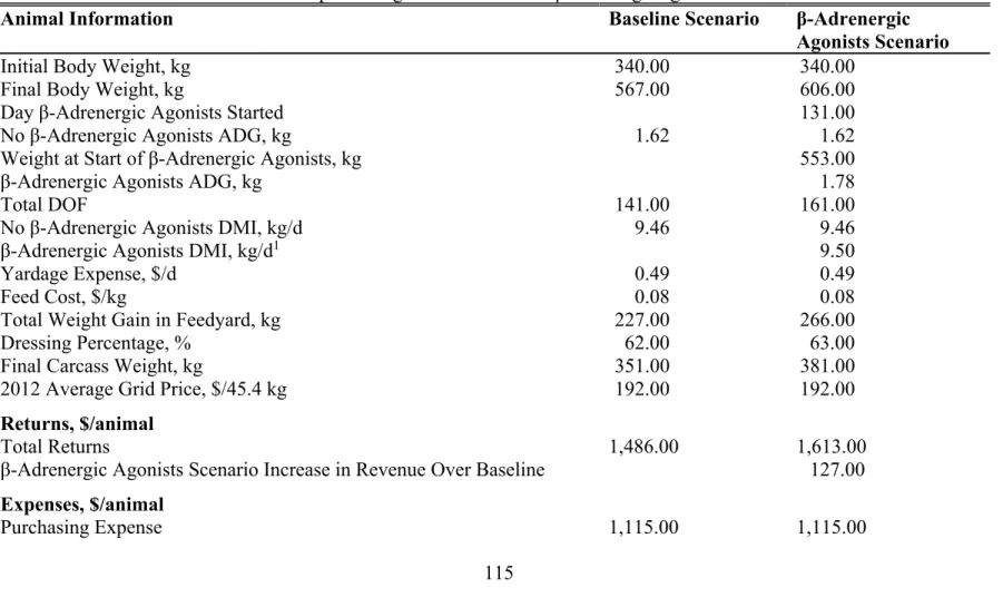
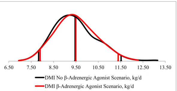
Cattle not consuming β-AA had a mean predicted DMI of 9.46 kg/d (ranging from 6.99 kg/d to 13.16 kg/d) and a mean predicted ADG of 1.62 kg/d (ranging from 1.22 kg/d to 2.03 kg/d). In the β-AA scenario, predicted DMI ranged from 6.93 to 12.29 kg/d with a mean of 9.50 kg/d. These figures represent an increase in DMI of 0.33% on average. Predicted ADG in the last 30 DOF in the BAA scenario was 1.78 kg/d and ranged from 1.36 to 2.75 kg/d, a predicted increase of 9.7% above baseline. Figure 1.2
31
shows the probability density functions (PDF) for DMI in both scenarios. Figure 1.3 displays the ADG PDFs for both scenarios. The PDFs are a visual representation of the distributions. The ADG PDF for the β-AA scenario in Figure 1.3 is shifted to the right compared to the no β-AA scenario ADG PDF. This indicates that for all probable outcomes, β-AA will increase ADG.
The estimated DMI and ADG values were subsequently used in the enterprise budgets. Table 1.1 contains the basic animal information as well as calculated values used to calculate the total returns and expenses, and ultimately, the difference in
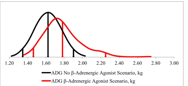
profitability between the baseline (no β-AA) and β-AA scenarios. The values presented in Table 1.1 are the average values from the simulation. Change in profitability ranges from a decrease of $-23.11/animal to $100.28/animal (Figure 1.4) with β-AA. A cumulative distribution function (CDF; Figure 1.5) of change in profitability for β-AA presents the probabilities on the Y-axis and the $/animal change in profitability on the X-axis. By tracing the line on the CDF graph the probabilities and $/animal change in profitability at the feedlot can be linked. For example, there is an 11.3% chance that the $/animal change in profitability will result in a decrease from using β-AA. Conversely, there is an 88.7% probability that the $/animal change in profitability will be positive when using β-AA.
The reduction in cost for the packer ranges from $0.12-$1.12/45.4 kg with an average of $0.63/45.4 kg (Figure 1.6).
The increase in profitability for the feedlot and reduction in cost for the packer are expected results, at the given price levels. While on β-AA, the animals have a
32
relatively unchanged DMI and increased ADG. So even though the animal may be on feed longer, the increase in revenues outweighs the increase in expenses. For the packer, their cost is reduced because the animal fed β-AA has a heavier HCW. Thus, it takes fewer animals to achieve the same number of total pounds as it would have with animals not fed β-AA. This reduces the fixed costs for the packer and environmental
consequences. For both the feedlot and packer, β-AA are a profitable technology. When β-AA are removed from beef cattle production there is a loss of a profitable technology. Additionally, HCW and dressing percentages decrease. These are shocks to the EDM, which disrupt the system. These shocks affect both the supply and demand at all market levels, for each meat product (beef, pork, poultry) because each market is interrelated. The ensuing results from the EDM represent the market system working back toward an equilibrium.
Initially, the removal of a profitable technology results in a higher cost of production. This reduces feedyard profit margin. If profit margins are to remain the same, then feeder cattle prices must go down (this represents a decrease in costs) and/or prices for slaughter cattle must increase (increase in revenue). Additionally, the removal of β-AA results in an immediate decrease in production (kg of beef), ceteris paribus, due to decreases in HCW and dressing percentage.
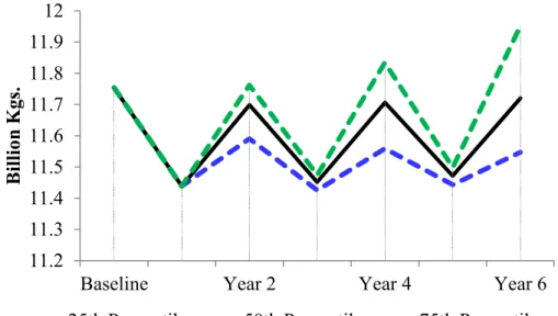
Fan graphs (Figures 1.7-1.14) start at the initial time point (baseline use) and continue outwards for six years. Lines on the fan graphs represent the twenty-fifth, fiftieth, and seventy-fifth percentiles and are the confidence intervals for the estimated means.
33
At the outset, quantity produced decreases in the retail, packer/processor, and feedlot market levels (Table 1.2). Feedlot cattle quantity differs from retail and
packer/processor quantity because feedlot quantity is calculated on a live animal basis. Feeder cattle quantity remains constant because the β-AA technology are employed after this phase. It is not until after market signals (price) are realized that the quantity of feeder cattle changes. Price of beef in the retail, packer/processor, and feedlot market levels initially increases because of the decrease in beef production. Quantity and price changes in pork and poultry markets are minimal in the beginning (because they have not yet had time to respond), but both variables increase as the market has time to adjust. Thus, when the response comes in the second period it is large, but generally declines in the following periods as the markets move towards equilibrium.
Generally, the largest percentage changes in prices and quantities are within the first two years because of the markets responses and biological nature of animals. Percentage changes in livestock and meat prices and quantities are presented in Table 1.3. These results are relative to a base of no β-AA removal. More meat (animals) cannot be produced instantly. Depending on the reproductive cycle of the animal it can take from a few months (poultry) to a few years (beef) for production to respond with more (or fewer) total animals produced (Stillman, Haley, and Mathews, 2009). This is seen in the feedlot and feeder cattle quantity fan graphs (Figures 1.11 and 1.13). Feedlot cattle quantity decreases in the first three years as a result of market price influences, the loss of a production increasing technology, and the fact that heifers must be retained as replacements to grow the beef cattle herd (Figure 1.11). Because more feeder cattle
34
cannot be immediately produced, the quantity produced is constant until the market is able to respond, but similarly heifers must be retained initially so the herd can be
expanded. Even as the price and quantity percent change diminishes year over year, the confidence intervals around these estimates widen. As estimates build out in time, error compounds, thus widening the confidence intervals.
As each year passes, the markets work toward equilibrium and the movements within the markets become smaller. Overall, beef quantities at all market levels, except feedlot, increase. Retail increases by 0.56%, packer/processor by 1.17%, feedlot cattle by -0.12%, and feeder cattle by 0.48%. Price decreases by 6.68% in retail, 6.32% in packer/processor, and 7.06% at feedlot. Feeder cattle price increases by 15.46% though. In the pork market quantities increase in all three market levels (4.12% in retail, 11.11% in packer/processor, and 2.48% in feeder). Price decreases at the retail and
packer/processor levels, but increases at the feeder level (-18.61% in retail, -19.00% in packer/processor, and 25.69% in feeder). For poultry quantity decreases at retail (-2.94%) and price increases slightly (0.46%). From the results, some economic welfare impacts can be inferred. The welfare impacts of β-AA removal were calculated for the initial time period. As prices increase and quantity decreases, consumer surplus
decreases by $0.910 billion at the beef retail level. Pork consumer surplus decreases by $0.019 billion at the retail level and poultry consumer surplus decreases by $0.373 billion at the retail level. Collectively, this results in a decrease of $1.302 billion in consumer surplus at the retail market level. Consumer surplus decreases for all three meat markets initially because the producers have not yet been able to respond to the
35
shock in the market. Initially, producer surplus will increase by these respective levels in each meat market. However, as the market works to expand and move towards equilibrium, producer surplus decreases and consumer surplus increases.
β-adrenergic agonists are a proven technology for increasing weight gain and decreasing feed intake in cattle. Depending on the market setting, β-AA are a profitable technology for feedlots and packing houses. However; animal welfare and consumer perception concerns resulted in ZH removal from the market in August 2013. This analysis examined the impact of the removal of all β-AA from beef cattle production. Removing β-AA from beef cattle production causes DMI to remain relatively unchanged (-0.33% on average), ADG to decrease (9.7% on average), and dressing percentage to decrease. This means that the cattle are less efficient at converting their feed, thus requiring more feed and time to reach the same weight. If time remains constant, then there is less meat produced when β-AA are not used. The implication is that the system is less sustainable because it requires more resources to produce less product. White and Capper (2013) report any production system that increases ADG or the finishing weight (FW) of an animal increases the sustainability. The increase in sustainability is achieved through decreases in feedstuff consumption, land use, water use, carbon footprint, and nitrogen and phosphorus excretion. β-adrenergic agonists are a critical part of a production system that helps make beef production more sustainable. Stackhouse-Lawson (2013) also pointed out that β-AA increase ADG, final BW, and HCW. Additionally, β-AA lower CH4, methanol, and NH3 emissions per kg HCW. So
36
(ammonia by 13%, methane and nitrous oxide by 31%; Stackhouse et al., 2012; Cooprider et al., 2011).
In this analysis, the removal of β-AA resulted in a change in profitability for feedlots ranging from $23.11 to -$100.28 per animal, with an 88.7% chance that profitability would be decreased by not using β-AA. The removal of β-AA also
increased costs for the processing sector by $0.63/45.4 kg on average. This reduction in profitability and increase in costs reduces the economic sustainability of these sectors. In 2007, Lawrence and Ibarburu estimated that β-AA reduced feedlot costs by $12-$13 per animal. Schroeder and Tonsor (2011) predicted an average net return from Zilmax® feeding of $21.08 per animal to feedlots, and a return of $31.68 per animal to the packer. White and Capper (2013) estimated an increase in income over costs of $0.24/d and $0.26/d for production systems that increased ADG or FW by 15% each, respectively, as compared to the control (average U.S. production). Cooprider, et al. (2011), estimated that the cost per kg of BW gain was increased by $0.23/kg for production systems not using feed additives or implants. Like here, Cooprider, et al. points out, increasing the cost of production reduces the economic sustainability of the enterprise. In every study, growth enhancing technologies have been shown to reduce costs or increase
profitability. The removal of growth enhancing technologies will lead to a reduction in domestic production, an increase in imports, and reduced competitiveness in the world market (Capper and Hayes, 2012). β-adrenergic agonists are a technology that improve the economic sustainability of the beef cattle industry.
37
Due to the changes from β-AA removal, in the long run beef consumers,
packer/processors, and feedlots face reduced prices and increased quantities of beef and animals, but both price and quantity of feeder calves increases (15.46% price, 0.48% quantity). The removal of β-AA creates a greater demand for feeder cattle because more animals are needed to maintain the same level of production, which drives an increase in demand for the number of head. Correspondingly, prices must increase to encourage the production of more feeder cattle. Additionally, price increases as well due to
competition among the feedyards for the feeder cattle. However, the increase in price of feeder calves contributes to the reduction in profitability for feedlots. The feedlot sector experiences both increased input prices (feeder calves) and reduced prices for their final product (fed cattle). This is a threat to the sustainability of the feedlot sector and may cause some feedlots to go out of business. So while increased prices may seem positive for the farm level, it may eventually lead them to have less (or no) feedlots to sell their product (feeder calves) to. Pork consumers, packer/processors, and growers will face increased quantities, with decreased prices for consumer and packer and increased prices for growers. Poultry consumers will see decreased quantities and increased prices.
Time and again, β-AA have been shown to improve both economic and environmental sustainability. The results of this analysis further support this idea. β -adrenergic agonists are a technology that allow there to be fewer in animals in
production to still obtain the same total kilograms of meat. This reduces the impact on the environment. As this analysis points out, the initial removal of β-AA reduces