Automatic detection of UXO magnetic anomalies using extended Euler deconvolution

Automatic detection of UXO magnetic anomalies

using extended Euler deconvolution

Kristofer Davis

, Yaoguo Li

, and Misac Nabighian

ABSTRACT

We have developed an algorithm for the automatic detec-tion of prospective unexploded ordnance共UXO兲anomalies in total-field or gradient magnetic data based on the concept of the structural index共SI兲of a magnetic anomaly. Identify-ing magnetic anomalies havIdentify-ing specific structural indices en-ables the direct detection of potential UXO targets. The total magnetic field produced by a dipolelike source, such as a UXO, decays with inverse distance cubed and therefore has an SI of three, whereas the gradient data have an SI of four. The developed extended Euler deconvolution method based on the Hilbert transform provides a reliable means for calcu-lating the spatial location, depth, and SI of compact and iso-lated anomalies; it has enabled us to perform automatic anomaly selection for further analysis. Our method first ex-amines the anomaly decay and selects possible UXO anoma-lies based on the expected SI. We refine the result further by post-Euler amplitude analysis using the relative source strength of the anomalies selected in the first stage. The am-plitude analysis statistically identifies weak anomalies that are due to noise in the data. This enhances the final result and eliminates automatic picks that fall within the noise level. We have demonstrated the effectiveness of the method using syn-thetic and field data sets.

INTRODUCTION

We develop a new method for detecting unexploded ordnance 共UXO兲anomalies in magnetic data. The method uses the concept of the structural index共SI兲as well as a statistical analysis of anomaly source strengths based on magnetic amplitude data. This method overcomes the drawbacks of simpler methods such as the threshold-ing of total-gradient data共often mistakenly referred to as the 3D ana-lytic signal兲and is more robust when dealing with interfering effects

of background geology and other noise in data sets. Our method is similar to that developed byBillings and Herrmann共2003兲that is based on a continuous wavelet transform using natural wavelets and examines the decay rate of anomalies. The ability to detect targets automatically by picking the anomalies that are caused by UXO-like objects is crucial in reducing false alarm rates and aiding in and speeding up discrimination through inversion共Billings, 2004兲.

Our detection method estimates location and, more importantly, the type of magnetic source that produced the anomaly. Any anoma-ly whose source appears to be dipolar is considered a potential UXO target based on the assumption that the majority of UXO act as a magnetic dipole to a high degree of approximation共e.g.,Butler et al., 2001;Sanchez et al., 2008兲. The total-field intensity of a magnetic dipole decays as inverse distance cubed and therefore has a structur-al index共SI兲of three. Geologic features have some elongation and a lower structural index than a dipole feature. Similar results can also be achieved using gradient data and an SI of four for a dipole anoma-ly.

Choosing solutions based on these criteria is not enough, howev-er. Therefore, we also introduce an amplitude analysis that derives anomalies’ relative source strengths from the amplitude data and then statistically identifies the targets. Only the anomalies with the highest source strengths are considered potential UXO because they naturally should have a larger magnitude of magnetization than sur-rounding geology. These results can then be used as initial guesses for dipole inversion or other discrimination techniques. First we will describe extended Euler deconvolution, then the methodology of how we use it, and finally amplitude analysis, as tools for automatic anomaly detection. After giving the numerical procedure, we illus-trate our method using synthetic and field data sets.

THEORY AND ALGORITHM Extended Euler deconvolution

Euler deconvolution was originally developed in exploration geo-physics for rapidly estimating the location and depth to magnetic or gravity sources. It is based on the fact that the potential field

pro-Manuscript received by the Editor 15 September 2008; revised manuscript received 9 October 2009; published online 21 April 2010.

1_{Colorado School of Mines, Department of Geophysics, Center for Gravity, Electrical, and Magnetic Studies, Golden, Colorado, U.S.A. Email: kdavis@}

mines.edu; [email protected]; [email protected].

© 2010 Society of Exploration Geophysicists. All rights reserved.

duced by many simple sources obeys Euler’s homogeneity equation. If a given component of the magnetic anomalous field⌬T共x,y,z兲 sat-isfies

⌬T共tx,ty,tz兲⳱tn_{⌬T共x,y,z兲, 共1兲}

wherenis the degree of homogeneity, then by differentiating equa-tion1with respect tot, it can be shown that

x⳵⌬T ⳵x Ⳮy ⳵⌬T ⳵y Ⳮz ⳵⌬T ⳵z ⳱n⌬T, 共2兲

wherex,y, andzare the field coordinates and the source is assumed to be at the origin. Equation2is known as Euler’s homogeneity equation共Hood, 1965兲or Euler’s equation. The degree of homoge-neity is source dependent and characterizes how fast the field de-creases as a function of distance to the source. For example, the total-field anomaly produced by a dipolar source decreases as inverse dis-tance cubed and the corresponding degree of homogeneity isn⳱ ⳮ3; a cylinder hasn⳱ⳮ2, and a thin dike hasn⳱ⳮ1. The same holds true for gradient anomalies as the degree of homogeneity for a dipolar source isn⳱ⳮ4; a cylinder,n⳱ⳮ3; and a thin dike,n⳱ ⳮ2.

Equation2can be used to estimate the source depth from magnet-ic data in three dimensions, whmagnet-ich gives rise to the method of Euler deconvolution共e.g.,Reid et al., 1990兲. Because the potential field decreases inversely proportional to the distance raised to some pow-er, the degree of homogeneity is nonpositive. The negative of the de-gree of homogeneity is defined as the structural index共SI兲and will be denoted asN. The structural index essentially characterizes the curvature of the magnetic anomaly. A faster decaying field has more high-frequency content and higher curvature, which corresponds to a higher SI; whereas a slower decaying field is smoother and has a correspondingly lower SI.

Assuming that the field due to a compact source located at 共xo,yo,zo兲is superimposed on a background field, we rewrite equa-tion2as

兺

␣

wherexirepresents the three orthogonal directionsx,y, andz; and␣ represents a constant background value, which is strongly coupled with the structural index. Equation3contains five unknowns:xo,yo,

zo,␣, andN. Due to the strong coupling between the variables␣and

N共Thompson, 1982兲, it is customary to assume an a priori value for

N and solve for the remaining four unknowns. The x-, y-, and

z-derivatives can be calculated using various algorithms depending on the distribution of original data. Applying equation3to a group of neighboring data points, we obtain a system of equations that can be solved in a least-squares sense for the source location共xo,yo,zo兲and the background level␣. The algorithm usually is applied to points within a window of a specified size. The a priori choice of a structural index has been the topic of much discussion in the literature because it is somewhat arbitrary, and the obtained solutions depend strongly on that choice.

Nabighian and Hansen共2001兲extend the work by Mushayande-bvu et al.共1999兲and show that the same Euler equation also holds true for the two components of the 3D Hilbert transforms of the field:

兺

兺

where Hx关⌬T兴 and Hy关⌬T兴 denote, respectively, the x- and

y-component of the 3D Hilbert transform共Nabighian, 1984兲applied to the field⌬T. In contrast with equation3, the equations4do not re-quire a background term because the Hilbert transform of a constant is equal to zero. The absence of a background term now allows for the direct evaluation of the structural indexN, and this leads to a more stable and versatile method of depth estimation and source lo-cation. Thus we now have an effective means to estimate not only the source location and depth but also, independently, its structural in-dex.

Automatic anomaly detection

The ability to estimate the structural index, instead of specifying it in advance, means that we can distinguish among different source types during the depth-estimation process. This enables us to identi-fy UXO responses among the interfering anomalies of geologic ori-gin. The majority of UXO items are predominantly dipolar sources. The corresponding total-field magnetic anomaly⌬Tis given by

⌬T共r兲⳱

␮

4

␲

·Bˆo, 共5兲

wheremis the dipole moment;Bˆois a unit vector along the direction of the ambient magnetic field; androandrare, respectively, the loca-tion of the dipole and the observaloca-tion point. It follows that the struc-tural index of a dipolar field is three. The same concept also applies to gradient data. For the gradient of the total field⳵⌬T/⳵xi, in the

xi-direction, the dipolar anomaly is given by

⳵⌬T ⳵xi 共r兲⳱

␮

␲

wherem,Bˆo,ro, andrare same as in equation5. The extra derivative introduced in equation6means that the structural index of the gradi-ent of a dipolar field is four. We will exemplify our proposed tech-nique on total-field magnetic data⌬T; to work with gradient data ⳵⌬T/⳵xi, one can exchange⌬Twith⳵⌬T/⳵xi, and change the corre-sponding SI.

The majority of geologic features have some elongation, and their magnetic anomalies would have a structural index less than that of a dipolar feature. Based on this observation, we have developed a method for automatically picking UXO anomalies using calculated structural indices. The central premise of the proposed method is that any compact source identified by extended Euler deconvolution as having a structural index close to three for total-field data, or four for gradient data, can be considered a potential UXO target and merits further investigation.

Equations4are applied throughout the entire data set within slid-ing windows. Each window yields a valid solution if there is a signif-icant magnetic anomaly within that window. The reliability of a so-lution often is affected by the choice of window size because a small window might not capture the anomaly pattern necessary for the cal-culation, and a too-large window might introduce interference from

adjacent anomalies. In general, one would use a larger window size for deeper sources and a smaller window size for shallower sources. For our application, we have chosen to use multiple window sizes to allow for the variable depths and sizes of UXO targets in an area.

The method first performs a sequence of Hilbert transform-based Euler deconvolutions using different window sizes on the data set, and obtains estimates of source locations and structural indices. It then examines the variation of the SI with window size and identifies the Euler solutions that yield SI values close to the target SI共 FitzGer-ald et al., 2004兲. Any anomalies with an SI close to the specified tar-get structural index, within a user-specified tolerance, would indi-cate a potential UXO target. Specifying a tolerance is necessary be-cause of the influence on the calculated SI by noise in the data and by all previous processing steps. The threshold should be above two for total-field data and above three for gradient data. The ideal SI from a cylinder would be at these values, and thus anything above it could be a potential dipole anomaly.

The noise in a data set can corrupt the signal that the extended Eu-ler deconvolution is searching for, and thus the accuracies of loca-tions, depths, and SI will decrease with the noise level共 Mushayan-debvu et al., 2001;FitzGerald et al., 2004兲. These values will be af-fected by the noise in the data set and will be closer to the theoretical SI values only for cleaner data. The results will also, in general, be more accurate for gradient data as the noise level often is significant-ly lower than in total-field data.

Numerical procedure

Assuming a gridded magnetic data set⌬T, the detection method begins by computing the two horizontal derivatives⳵⌬T/⳵x and ⳵⌬T/⳵yusing stabilized numerical differentiation operators to re-duce noise共Lanczos, 1988兲. The stable numerical differentiation first obtains a least-squares fit of a parabola through five data points and then finds the derivative of the parabolic function. This method suppresses the adverse effect of high-frequency noise in the data. The vertical derivative⳵⌬T/⳵zthen is computed in the Fourier do-main through the use of 3D Hilbert transform relations共Nabighian, 1984兲: ⌬T˜ z⳱H˜x⌬T˜xⳭH˜y⌬T˜y 共7兲 ⳱ⳮ i

␻

冑

␻

␻

␻

冑

␻

␻

where␻x, and␻yare the wavenumbers in thex- andy-directions, re-spectively, of the 2D Fourier transform; and⌬˜Tx,⌬T˜y, and⌬T˜zare the Fourier transforms of thex-,y-, andz-derivatives of the magnetic anomaly, respectively. The two components of the 3D Hilbert trans-form of the original magnetic anomaly and its three spatial deriva-tives allow us to obtain the eight quantities related to the magnetic anomaly required in the equations4. The derivatives of each Hilbert transform component in the equations4are obtained by applying the Hilbert transform to each corresponding derivative of the original anomaly.

Using the eight calculated quantities outlined above, equations4

now can be solved in each window using least squares. As mentioned previously, a range of different window sizes is used. This step yields the source-location estimates共xo,yo,zo兲and the structural indexNfor the particular source. From the set of windows centered at the same location, we find the one solution whose structural indexNis closest

to 3 for total-field data or 4 for gradient data. This solution is taken as the best solution associated with the set of windows centered at a common point. If a solution exists and the structural index is greater than a threshold value, we assume that the algorithm has detected a possible UXO-like anomaly. The corresponding location provides a first-order estimate for the dipole position. Performing this proce-dure on a data set produces a map of detected anomalies and their source locations. The horizontal locations can be used subsequently to help extract individual anomalies for determining source parame-ters through dipole inversion or other discrimination techniques.

Synthetic examples

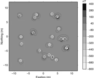
We now demonstrate the method with a synthetic data set. For clarity, we designed this example only to illustrate the basic concepts of the method and to address other aspects of practical application. The synthetic data were generated from 20 dipoles with random lo-cations, orientations, depths, and dipole moments共Figure1兲. The depths range from 0.3 to 0.8 m, with dipole inclinations ranging be-tweenⳮ90° and 90°, declination betweenⳮ180° and 180°, and di-pole moments varying between 0.1 and 0.5 Am2_{. The ambient} mag-netic field is assumed to have an inclination of 65° and a declination of 25°. These 20 dipole sources were used to produce the total-field anomaly according to equation5at 0.1-m grid spacing as well as their horizontal and vertical gradients.

We first apply our detection algorithm to the total-field anomaly over 12 window sizes varying between 3 and 25 grid points in each direction. Corresponding to each magnetic anomaly, a large number of Euler solutions were generated from windows that were able to calculate a structural index close to three from the dipole anomalies. The solutions in such a group differ only slightly from each other. Assuming all solutions within a 0.5-m radius come from the same target, we clustered the solutions after thresholding the SI for the en-tire data set and obtained 20 distinct detected anomalies. All detected anomalies have an SI greater than 2.5. Of these 20 solutions, 19 coin-cide with true anomalies in the data set, and one is located between

10 5 0 –5 –10 –10 –5 0 5 10 400 280 160 40 –80 –200 –320 –440 –560 –680 –800 Northing (m) Easting (m) nT

Figure 1. The total-field response for 20 randomly oriented dipoles. The⫹indicates where extended Euler deconvolution picked poten-tial UXO anomalies. One detection was a false positive, and the al-gorithm missed one dipole feature.

two adjacent anomalies. Thus, we have correctly detected 19 out of 20 anomalies, missed one anomaly, and produced a single false alarm. The result is shown in Figure1, where we posted the detection result and the known dipole locations over the grayscale contours of magnetic anomaly.

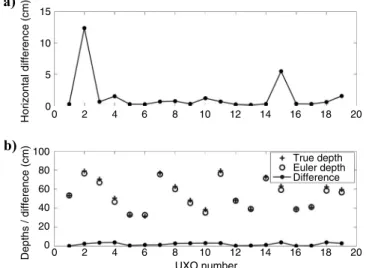
We also compare thex-ylocations and depths from the Euler solu-tions with the true values in Figure2. The maximum difference in the

x-yplane was 12 cm radially. The maximum difference between the true and calculated depths was 4 cm. The results have yielded a first-order approximation to dipole locations in three dimensions. Figure

3shows the SI for the detected anomalies. Only five of these anoma-lies actually achieved the exact dipole SI of 3.0. This means a lower, fractional SI should be used for the detection algorithm, particularly

in the presence of noise. The threshold, however, still should be above the SI of an ideal cylinder, 2.0, to maintain the assumption of dipole features.

We note that the missed anomaly in this example was a weak posi-tive anomaly juxtaposed between a weak and a strong negaposi-tive anomaly. This seemed to have confused the detection algorithm be-cause the interference by the two adjacent anomalies be-caused the cal-culated decay rate to be much smaller. The false anomaly occurred between two closely spaced anomalies. This solution was produced from a large window size, causing the algorithm to have difficulties recognizing the presence of two neighboring anomalies because the Euler solution assumes only one source per window. Larger window sizes are still necessary, however, to observe larger anomalies.

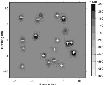
We now turn to the gradient of the synthetic data to examine how the results would differ. The vertical gradient of the same data set is used and extended Euler deconvolution applied共Figure4兲. The re-sults are similar to the total-field rere-sults; however, the false anomaly is no longer present. Euler deconvolution successfully detected 19 targets and no false positives. The same results also were achieved with the horizontal gradient共Figure5兲. There were no false posi-tives, and the only target missed was the same target as missed by the total-field data with a weak magnetic positive between weak and strong magnetic negatives. An SI threshold of 3.5 was used for both gradient data sets.

The synthetic data sets have demonstrated the concept of extend-ed Euler deconvolution and the automatic picking of UXO-like anomalies. Although no noise was present, the algorithm missed an anomaly because of the overlapping signals from multiple surround-ing anomalies and had only one false alarm. The missed anomaly in all three data sets illustrates one potential weakness of the algorithm: The extended Euler method might have difficulties when multiple anomalies are close together. The picks it did make, however, had high structural indices, and the calculated 3D locations of the dipoles were quite accurate. The nature of the algorithm allows for the auto-matic picking of dipolelike anomalies for large data sets with

mini-15 10 5 0 0 2 4 6 8 10 12 14 16 18 20 Horizontal difference (cm) 0 2 4 6 8 10 12 14 16 18 20 100 80 60 40 20 0 Depths / difference (cm) UXO number True depth Euler depth Difference

a)

b)

Figure 2. Comparison between true and estimated dipole locations. 共a兲The horizontal distance between the true and predicted dipoles. 共b兲The true and predicted depths and the difference between the two. The vertical axes in共a兲and共b兲are in units of cm. Only the solu-tions that corresponded to true targets were used in the comparison.

3 2.95 2.9 2.85 2.8 2.75 2.7 2.65 2.6 2.55 2.5 0 2 4 6 8 10 12 14 16 18 20 Detected anomalies Calculated Sl

Figure 3. A histogram of structural indices from detected anomalies of the synthetic total-field data. Only 5 of the 20 had an SI of 3.0, and thus a threshold of 2.5 was used. The threshold should still be above the SI of an ideal cylinder, 2.0, to keep the assumption of the dipole features intact. 10 5 0 –5 –10 –10 –5 0 5 10 400 280 160 40 –80 –200 –320 –440 –560 –680 –800 Easting (m) Northing (m) nT/m

Figure 4. The vertical gradient response of the same 20 randomly oriented dipoles as in Figure1. The⫹indicates picked potential UXO anomalies. The extended Euler deconvolution correctly picked 19 anomalies and missed one.

mal human interaction. This will significantly reduce processing time in the detection stage and allow one to expend more time on dis-crimination.

REDUCTION OF FALSE ALARMS

The results in the synthetic examples amply illustrated the con-cept of a Euler deconvolution-based detection algorithm and its effi-cacy. In practical applications, however, noise will strongly influ-ence the performance of any detection algorithm and lead to false alarms. Thus, a practically applicable algorithm must be able to deal with noise effectively and reliably. Data noise in UXO magnetic data can be generated during the acquisition stage or come from geology. Although established quality control and assurance procedures might significantly limit the acquisition error and its adverse effect on the automated detection method, geologic noise will always be present. When the wavelengths of geologic noise are comparable with those of UXO anomalies, the noise poses a severe challenge. We examine the issue here and develop a statistical method for re-ducing false alarms based on amplitude analysis.

For this purpose, we use a subset of total-field magnetic data from the former Camp Sibert in Gadsden, Alabama共color image in Figure

6兲. The data set was acquired as a part of the Environmental Security Technology Certification Program 共ESTCP兲 Project MM-0533 共Nova Research Inc., 2007兲. There are clear magnetic anomalies produced by UXO items and surface clutter as well as by geologic features that are comparable in scale length and shape. This data set typifies geologic noise in UXO magnetic data and the associated dif-ficulties in detection and discrimination.

It is instructive to examine the data image in Figure6and envision the difficulties of picking potential anomalies by eyesight or thresh-olding total gradients. The number of probable anomalies and the in-fluence of geologic noise likely would defeat such an effort. The dif-ficulty is illustrated by the large number of anomalies picked by the simple application of the proposed detection algorithm. When ap-plying our automated detection algorithm in its simple form, we chose a threshold ofN⬎2.2 for the SI and clustered the solutions within a 1-m radius共Figure6兲. This resulted in 161 anomalies in the area 30 m by 30 m. Only a few of these anomalies are clearly UXO related. Although the majority of the remaining anomalies are dipo-lar in shape共and have high structural indices兲, they are manifesta-tions of the noise within the data set.

The cause of these false alarms lies in the fact that the extended Euler deconvolution solves for the source location and structural in-dices based on the decay of the field within the window regardless of amplitude. The rate of field decay is quantified through the shape of the magnetic anomaly alone. Spatial variations in data due to the presence of noise can appear partially dipolar and yield high struc-tural indices, which lead to false alarms. This is compounded by the need for a lower SI threshold. The field data are contaminated by noise and usually undergo several standard processing steps and sta-bilized numerical differentiation prior to Euler deconvolution. The cumulative effect of noise and low-pass filtering tends to reduce the SI of an anomaly from its theoretical value, as we have observed in this data set and all other data sets we have worked with. To account for the reduction of calculated SI, we choose a lower threshold value of 2.2 for the data set so as to capture all UXO anomalies. The use of a lower threshold tends to increase false detections. Thus, further processing is required to winnow these false alarms.

To achieve the reduction, we turn to the complementary

informa-tion that was neglected in the Euler deconvoluinforma-tion: the amplitudes of magnetic anomalies. We have observed that the strengths of magnet-ic anomalies are in general weaker for surface clutter and small-scale geologic features. This reflects the fact that modern magnetic data are generally of high quality, and false anomalies due to survey er-rors cannot be too large in amplitude. Furthermore, these features are usually small in physical size or weak in magnetization. It follows that knowledge of the source strength will provide additional infor-mation for us to distinguish between strongly magnetic UXOs and

10 5 0 –5 –10 –10 –5 0 5 10 400 280 160 40 –80 –200 –320 –440 –560 –680 –800 Easting (m) Northing (m) nT/m

Figure 5. The horizontal共north-south兲gradient response of the 20 random dipoles. The⫹indicates picked potential UXO anomalies. Similar to the results from the vertical gradient, the extended Euler deconvolution correctly picked 19 anomalies and missed one.

30 25 20 15 10 5 0 465.69 5.39 3.41 2.44 1.71 1.10 0.58 0.06 –0.44 –0.96 –1.48 –2.05 –2.78 –3.83 –5.64 –210.77 0 5 10 15 20 25 30 nT Northing (m) Easting (m)

Figure 6. Initial Euler detection for a subset of field data from Camp Sibert. The color image with the corresponding color bar shows the total-field anomaly over an area 30⫻30 m. Superimposed on the data image are⫹symbols indicating the anomalies detected with an SI threshold of 2.2. A cluster radius of 1 m was used. The algorithm picked a total of 161 anomalies. All of the UXO anomalies were identified correctly, but there were a large number of false alarms clearly associated with background noise.

other sources. Strictly speaking, one might desire to carry out para-metric inversion to recover source strengths, i.e., dipole moments, of all anomalies detected in the first stage. However, that would be an expensive proposition not justified for anomaly detection. We choose to rely on the amplitude data computed from the total-field data as a proxy to the source strength.

We define the amplitudeAas the magnitude of the anomalous field vectorBជa: A⳱兩B

ជ

冑

whereBax,Bay, andBazare, respectively, the three components of the anomalous fieldBជa. The measured total-field anomaly is the

projec-tion ofBជaonto the inducing field direction. The amplitude data con-stitute an approximate envelope of the total-field anomaly over all possible magnetization directions共Nabighian, 1972;Shearer, 2005兲, and the peak is centered nearly directly above the corresponding source in three dimensions. Furthermore, the amplitude peak value is proportional to source strength and inversely proportional to the depth raised to the power of the structural indexN. Consequently, we can obtain a relative measure of the source strengths by examining the peak amplitude of each anomaly detected by Euler deconvolu-tion. Thus, we define the relative source strength as

兩m兩⬀hNA共xo,yo兲, 共10兲

where兩m兩is the magnitude of the dipole moment,his the depth of the dipole, andA共xo,yo兲represents the magnetic amplitude data at the location共xo,yo兲of the detected anomaly.

Scaling the amplitude data by the rate of decay using the structural index, which is equal to three for total-field data, is equivalent to re-moving the decay of the field with distance. A similar approach is used bySinex et al.共2005兲to evaluate strengths of different field components in UXO discrimination. For each anomaly, we choose to use the mean depth of the clustered Euler solutions. We can use ei-ther the theoretical value of three or the SI calculated by extended Euler deconvolution; numerical tests have indicated that the final de-tection results do not differ significantly.

Generating these relative source strengths is straightforward and computationally inexpensive. It requires three linear transforms of the total-field anomaly to obtain the three orthogonal components in equation9. This step is accomplished in the wavenumber domain 共Pedersen, 1978兲. Scaling the amplitude data at each detected anom-aly location according to equation10then yields relative source strengths for all dipole anomalies from the Euler picks.

The relative source strengths of the Euler solutions shown in Fig-ure 6 are summarized in Figure 7, which displays the source strengths in ascending order. It is observed that the anomalies pre-dominantly have somewhat weak source strengths that are nearly zero, and only a few anomalies are strong and deviate from the ma-jority. Closer inspection of the locations of these anomalies shows that the strong sources are indeed generally associated with the UXO anomalies identifiable by visual inspection, and the weaker ones are scattered in the portion of the data map where the signal-to-noise ra-tio is low.

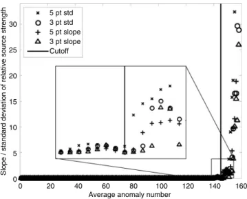
The problem of distinguishing between UXO anomalies and false alarms now becomes one of deciding a break point between these two groups of sources. We examined two criteria. The first is the rate of increase in sorted source strength as a function of the index calcu-lated over a running window; and the second is the standard devia-tion of source strength over the same window. Figure8shows the rate of increase and standard deviation calculated using a three-point and a five-point window, respectively. Both criteria seem to perform well in detecting the break point. We discard the Euler solutions be-fore the break point; these solutions lie within the noise and in most cases would not be considered UXO. This process winnows most of the Euler picks and identifies 16 remaining ones as having signifi-cant strengths.

To further confirm the validity of the criteria, we have examined the anomaly depths estimated by the Euler deconvolution. All 16 re-maining anomalies are located below the ground surface. It is reas-suring to note that all discarded anomalies lie near the ground sur-face. Therefore, a simple threshold based on the condition that the source depth must be greater than the observation height above the 100 90 80 70 60 50 40 30 20 10 0 0 20 40 60 80 100 120 140 160 180 Anomaly index Relative source strength

Figure 7. Sorted relative source strengths of all anomalies detected in Figure6. The vertical axis shows the source strength, and the hori-zontal axis is the anomaly index.

30 25 20 15 10 5 0 20 40 60 80 100 140 0 120 160

Average anomaly number

S lope / standard deviation o f relative source strength 5 pt std 3 pt std 5 pt slope 3 pt slope Cutoff

Figure 8. Rates of increase and standard deviations of source strengths共Figure7兲 calculated within three-point and five-point windows, respectively. These curves all show a clear break point be-tween the anomalies within the noise level and those standing out. The cutoff level is chosen to be the first large rate of strength increase or standard deviation. The inset zooms in around the point chosen.

ground would have winnowed some false alarms. However, ampli-tude analysis still is needed to remove those false alarms appearing to be just below the ground surface and having low relative source strengths.

The final 16 potential UXO anomalies chosen through amplitude analysis following the extended Euler deconvolution are shown in Figure9. All could be interpreted as potential UXO anomalies be-cause of the dipole nature of each shape. Dig results共prior to this work兲from the same area targeted 10 anomalies, four of which were actually UXO and six others scrap metal共Figure9兲. Euler solutions existed for eight anomalies from the dig results, meaning only half of the dipole anomalies chosen by the algorithm were not of interest in discrimination techniques. The Euler results did not miss any UXO, and the average of the structural indices for the UXO anomalies was 2.6. Thus, we can state confidently that the automated detection al-gorithm with the added amplitude analysis has worked well in this case.

CONCLUSIONS

We have developed an algorithm for automatically detecting UXO anomalies by using extended Euler deconvolution based on Hilbert transforms. The central premises of the algorithm are two-fold. First, extended Euler deconvolution of magnetic data can yield a reliable estimate of an anomaly’s structural index and location; and second, any magnetic anomaly whose structural index is close to that of a dipole共i.e., three for total-field data and four for gradient data兲is a compact source and constitutes a possible UXO anomaly requiring further analysis. We have successfully demonstrated the algorithm’s performance using synthetic total-field and gradient data without noise. Results have shown that the majority of buried UXO targets can be detected.

The first component of the algorithm performs extended Euler de-convolutions with a range of window sizes and solves for the source location and structural index. All results above the user-specified threshold of the structural index are collected as viable solutions for

UXO detection. It is important that the user select a threshold to cap-ture all of the dipole feacap-tures within the data set. In general, several solutions will be present around each dipole feature, so they are clus-tered into a mean solution within a given radius. It is noteworthy that this step assumes a single magnetic anomaly within each window. Thus, multiple UXO targets within the window area will affect cal-culations adversely.

The estimated horizontal and vertical locations of the detected anomalies in the synthetic examples agree well with the true loca-tions. The estimated dipole locations, therefore, provide a good first estimate for subsequent quantitative analyses. For example, these locations can then be used as an initial guess of the dipole location in an inversion for discrimination.

The second component of the algorithm performs amplitude anal-ysis to reduce false alarms in a noisy environment. The presence of background geologic anomalies and acquisition noise will influence the solution as expected. The criterion of looking for high structural indices can potentially lead to a large number of false alarms associ-ated with background noise, as exemplified by the field data exam-ple. To counteract this, we have developed an amplitude analysis technique that distinguishes between strong UXO anomalies and those caused by data noise and geologic noise. The analysis statisti-cally examines the variation of relative source strengths derived from the magnetic amplitude and Euler structural index, and detects the break point. Any anomalies whose strength falls below the break point are considered to be in the noise range and discarded. This ap-proach worked well in the field data example.

It is important to note that our algorithm is not a discrimination technique, but a tool for automatically choosing potential UXO anomalies based on the assumption that a UXO anomaly has a dipo-lar shape. The anomalies require further investigation. The locations of the buried anomalies are only approximations calculated through extended Euler deconvolution, and the SI tend to be smaller than the theoretical value due to the effect of noise and data processing. Nonetheless, our algorithm is able to narrow the possible anomalies to a small set and provide users with enough semiquantitative pa-rameters so that an efficient qualitative discrimination might be at-tempted.

Overall, the algorithm provides a much-needed alternative solu-tion for prediscriminasolu-tion anomaly detecsolu-tion so that large data sets can be processed automatically. The corresponding estimates of lo-cations and depths of detected anomalies will provide a reliable ini-tial guess for subsequent quantitative inversion used in discrimina-tion.

ACKNOWLEDGMENTS

We thank Don Yule for his support that initiated the project. We also thank Len Pasion and Todd Meglich for helpful discussions on the Camp Sibert data set. This research was supported in part by a grant from the Engineer Research and Development Center共ERDC兲 and by the Strategic Environmental Research Development Pro-gram共SERDP兲through project MM-1638.

REFERENCES

Billings, S. D., 2004, Discrimination and classification of buried unexploded ordnance using magnetometry: IEEE Transactions on Geoscience and Re-mote Sensing,42, 1241–1251.

Billings, S. D., and F. Herrmann, 2003, Automatic detection of position and depth of potential UXO using a continuous wavelet transform: Proceed-30 25 20 15 10 5 0 0 5 10 15 20 25 30 465.69 5.39 3.41 2.44 1.71 1.10 0.58 0.06 –0.44 –0.96 –1.48 –2.05 –2.78 –3.83 –5.64 –210.77 Easting (m) Northing (m) nT

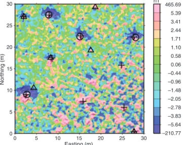
Figure 9. The final 16 Euler solutions共⫹兲obtained through source-strength analysis, cleared UXOs共䊊兲, and cleared non-UXO共䉭兲 anomalies. The two non-UXO items cleared from discrimination methods were initially picked by the algorithm, but then discarded during the amplitude analysis.

ings of the SPIE Technical Conference on Detection and Remediation Technology for Mines and Minelike Targets, 5089, 1012–1022.

Butler, D., P. J. Wolfe, and R. O. Hansen, 2001, Analytical modeling of mag-netic and gravity signatures of unexploded ordnance: Journal of Engineer-ing and Environmental Problems,6, 33–46.

FitzGerald, D., A. B. Reid, and P. McInerney, 2004, New discrimination techniques for Euler deconvolution: Computers and Geosciences,30, 461–469.

Hood, P., 1965, Gradient measurements in aeromagnetic surveying: Geo-physics,30, 891–902.

Lanczos, C., 1988, Applied analysis: Courier Dover Publications.

Mushayandebvu, M. F., P. van Driel, A. B. Reid, and J. D. Fairhead, 1999, Magnetic imaging using extended Euler deconvolution: 69th Annual In-ternational Meeting, SEG, Expanded Abstracts, 400–403.

——–, 2001, Magnetic source parameters of two-dimensional structures us-ing extended Euler deconvolution: Geophysics,66, 814–823.

Nabighian, M. N., 1972, The analytic signal of two-dimensional magnetic bodies with polygonal cross-section: Its properties and use for automated anomaly interpretation: Geophysics,37, 507–517.

——–, 1984, Toward a three-dimensional automatic interpretation of poten-tial field data via generalized Hilbert transforms: Fundamental relations: Geophysics,49, 780–786.

Nabighian, M. N., and R. O. Hansen, 2001, Unification of Euler and Werner

deconvolution in three dimensions via the generalized Hilbert transform: Geophysics,66, 1805–1810.

Nova Research Inc., 2007, Environmental Security Technology Certification Program共ESTCP兲technology demonstration data report; ESTCP UXO discrimination study; MTADS demonstration at Camp Sibert magnetome-ter/EM61 MkII/GEM-3 arrays: ESTCP Project MM-0533.

Pedersen, L. B., 1978, Wavenumber domain expressions for potential fields from arbitrary 2-, 2 1₂-, and 3-dimensional bodies: Geophysics, 43, 626–630.

Reid, A. B., J. M. Allsop, H. Granser, A. J. Millett, and I. W. Somerton, 1990, Magnetic interpretation in three dimensions using Euler deconvolution: Geophysics,55, 80–91.

Sanchez, V., Y. Li, M. N. Nabighian, and D. L. Wright, 2008, Numerical modeling of higher order magnetic moments in UXO discrimination: IEEE Transactions on Geoscience and Remote Sensing,46, 2568–2583. Shearer, S., 2005, Three-dimensional inversion of magnetic data in the

pres-ence of remanent magnetization: M.S. thesis, Colorado School of Mines. Sinex, D., Y. Li, and D. Yule, 2005, Improving UXO discrimination using

magnetic quadrupole moments: 75th Annual International Meeting, SEG, Expanded Abstracts, 680–683.

Thompson, D. T., 1982, EULDPH: A new technique for making computer-assisted depth estimates from magnetic data: Geophysics,47, 31–37.