Audio Compression Codec Using a Dynamic Gammachirp Psychoacoustic Model And a D.W.T Multiresolution Analysis

Audio Compression Codec Using a Dynamic

Gammachirp Psychoacoustic Model And a D.W.T

Multiresolution Analysis

Khalil Abid

National Engineering School of Tunis ( ENIT ) Laboratory of Systems and Signal Processing (LSTS)

BP 37, Le Belvédère 1002, Tunis, Tunisia [email protected]

Kais Ouni and Noureddine Ellouze

National Engineering School of Tunis ( ENIT ) Laboratory of Systems and Signal Processing (LSTS)

BP 37, Le Belvédère 1002, Tunis, Tunisia

Abstract—Audio compression algorithms are used to obtain

compact digital representations of high-fidelity audio signals for the purpose of efficient transmission over larger distances and storage. This paper presents an audio coder for real-time mutimedia applications. This coder applies a discrete wavelet transform to decompose audio test files into subbands to eliminate redundant data using spectral and temporal masking properties. This architecture is combined with a psychoacoustic model characterised by an external and middle ear model as a first part and a dynamic Gammachirp filter as a second part whose connections are selected in order to come close to the critical bands of the ear. Experimental results show the best performance of this architecture

Keywords-Audio Compressiont; Discrete Wavelet Transform; Psychoacousic Model; External and Middle Ear Model; Dynamic Gammachirp Filter Bank;MUSHRA listening test;

I. INTRODUCTION

Although wireless communication has played a great role in our lifestyle, transmission of high fidelity audio signal wirelessly at a reasonable cost is still challenging. Presently available audio coding techniques aim at reducing bitrate and put less concern on complexity and efficient wireless transmission. Such audio CODECs like ISO/MPEG and AAC [9] are suitable for non real−time applications and audio archive. In audio coding there is a trade-off between the compression ratio and reconstruction quality. Higher compression ratios imply more degradation on the sound quality when reconstructed. Any compression scheme should consider these facts and should also provide a good control mechanism to use the limited bandwidth and maintain acceptable quality, keeping in mind the computational complexity. The variability of audio compression techniques offer various compressed audio quality, amount of data compression and levels of complexity. Despite this variability the present audio encoders are based on the Fourier transform

which is localised only in frequency unlike the wavelet transform. This technique is a time-frequency localization analysis method for non-stationary signal and has been identified as an effective tool for data compression. The window width of wavelet analysis is adjustable. It is shorter at higher frequencies and larger at lower frequencies. The time-frequency characteristic of a wavelet filter bank is a natural match to some of the properties of wideband speech and audio signal. This paper proposes an audio coding scheme based on subband analysis using the discrete wavelet transform and adopts an analysis of the frequency bands that come closer to the critical bands of the ear . Our goal is not to propose a new wavelet type but to apply the wavelet formalism for speech/music discrimination. Our motivation to apply wavelets to speech/music discrimination is due to their ability to extract time-frequency features and to deal with non-stationary signals [8]. This paper is arranged as follows: Section 2 elaborates the proposed D.W.T encoder. Section 3 will focus on the the Gammachirp model. Section 4 aims at presenting the architecture of the psychoacoustic model using the dynamic Gammachirp wavelet. Experimental results are shown in section 5. A sound quality evaluation will be presented in section 6. Finally, a hardware implementation of the D.W.T CODEC will be carried out to conclude this work.

II. THE D.W.T AUDIO ENCODER

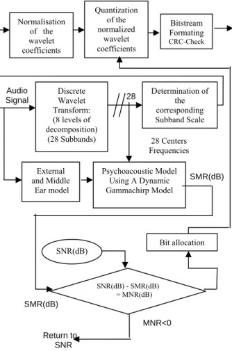
The architecture of the classical perceptual MPEG1 audio compression [1] is shown in the following Figure 1. This model use signal analysis, psychoacoustic models, bit allocation and coding blocks. At the ISO/MPEG1 layer III (MP3) coding scheme [1], the time to frequency mapping block includes a polyphase analysis filter bank followed by decimation of a factor of 32 [1], feeding a modified discrete cosine transform (MDCT) [1] and adaptive segmentation block, also connected with the psychoacoustic model. The bit allocation block includes block companding, quantization and Huffman coding [1].

Figure 1. The classical MPEG1 audio encoder

A. Stucture of The D.W.T Encoder

This section explains the structure of the proposed D.W.T codec using as input wave file audio. Each file has the following properties (Sample rate Fe=44.1Khz and Bitrate=705Kbits/s) and is troncatured at 1024 samples. The encoder is based on discrete wavelet transform D.W.T, which has strong relations with subband analysis and filter bank.

Figure 2. The D.W.T Encoder

The D.W.T is applied to the audio input signal with 8 levels of decomposition, thus concentrating energy in lower frequency bands (higher levels). This part decomposes and transforms the audio frame [17] into wavelet domain. The decomposition tree consists of 28 subbands chosen to resemble the critical band [11][19] of human hearing as depicted in Figure 3. Each subband will be quantized according to the signal to mask ratio (SMR) calculated by the dynamic Gammachirp Psychoacoustic Model .

Figure 3. The discrete wavelet transform repartition

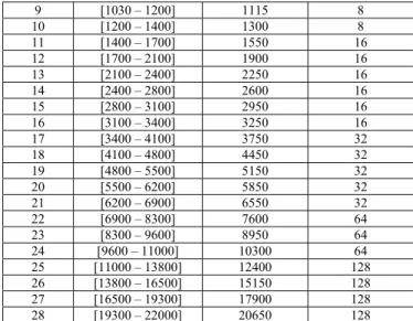
TABLE I. THE D.W.T SUBBAND REPARTITION

Subband _[ min F -max F ] (HZ) Center Frequency 0 f (Hz) Number of samples 1 [0 – 90] 45 4 2 [90 – 170] 130 4 3 [170 – 260] 215 4 4 [260 – 340] 300 4 5 [340 - 520] 430 8 6 [520 – 690] 605 8 7 [690 – 860] 775 8 8 [860 – 1030] 945 8 Normalisation of the wavelet coefficients Quantization of the normalized wavelet coefficients Bitstream Formating CRC-Check Discrete Wavelet Transform: (8 levels of decomposition) (28 Subbands) Determination of the corresponding Subband Scale External and Middle Ear model Psychoacoustic Model Using A Dynamic Gammachirp Model SNR(dB) - SMR(dB) = MNR(dB) SNR(dB) Audio Signal SMR(dB) SMR(dB) Bit allocation MNR<0 Return to SNR 28 28 Centers Frequencies Filter Bank (32 equal subbands) Quantization and Coding Classical Psychoacoustic Model Side information Bitstream Formating Signal.wav Audio encoded signal

9 [1030 – 1200] 1115 8 10 [1200 – 1400] 1300 8 11 [1400 – 1700] 1550 16 12 [1700 – 2100] 1900 16 13 [2100 – 2400] 2250 16 14 [2400 – 2800] 2600 16 15 [2800 – 3100] 2950 16 16 [3100 – 3400] 3250 16 17 [3400 – 4100] 3750 32 18 [4100 – 4800] 4450 32 19 [4800 – 5500] 5150 32 20 [5500 – 6200] 5850 32 21 [6200 – 6900] 6550 32 22 [6900 – 8300] 7600 64 23 [8300 – 9600] 8950 64 24 [9600 – 11000] 10300 64 25 [11000 – 13800] 12400 128 26 [13800 – 16500] 15150 128 27 [16500 – 19300] 17900 128 28 [19300 – 22000] 20650 128

In order to evaluate the proposed D.W.T repartition, we compared the positions of its center frequencies with the real one. As shown in Figure 4 the second repartition using D.W.T has approximately the same repartition.

101 102 103 104 0 10 20 30 40 Frequency (Hz) Ba rk

Real Centers Frequencies repartition

101 102 103 104 0 10 20 30 40 Frequency (Hz) Ba rk

Centers Frequencies repartition using The proposed DWT

Figure 4. Comparison between the real and D.W.T centers frquencies repartition

To avoid cases where wavelet coefficients exceeded the number of samples in time domain, each frame is viewed as periodic. In order to decompose frame and down-sampling by

two at each level of the tree, we used the following equation:

0 1 0 1 0 1 _{0 1 0 1} 2 2 ( j , j ) ( i ) ( k , k ) n n i n j n j n _{k k} M S W Samp Xs Y f g          _{     }   (1) Where: 1 1 3 2 1 3 2 1 2 1 3 2 1 3 0 1 2 0 1 2 0 0 0 1 0 1 0 1 0 1 ( ) 0 0 0 0 0 0 0 0 0 0 0 0 0 0 0 0 ( , ) 0 0 0 0 0 0 M M M M M M M M M M M M M M M M j j j j nxn S S S S W W W W S S S S W W W W M S W S S S S S W W W W W                                                                               (2) 0 1 2 3 4 0 1 5 2 1 1 ( i ) i n n n n X s X s X s X s X s S a m p X s X s X s X s                                     (3) 0 0 1 1 2 2 3 0 1 0 1 2 2 3 1 2 1 2 1 ( _k , _k ) n n k k n n n f g f g f g Y f g f g f g                                                  (4)

 The number of samples (

Xs

) is equal to n.

 The number of wavelet function coefficients (W) is equal to m

 The number of scaling functions (

S

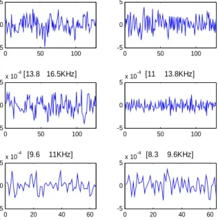
) is equal to m 0 50 100 -5 0 5x 10 -4 Details [19.3 22KHz] J=1 0 50 100 -5 0 5x 10 -4 Approximations [16.5 19.3KHz] 0 50 100 -5 0 5x 10 -4_{[13.8 16.5KHz]} J= 2 0 50 100 -5 0 5x 10 -4 _{[11 13.8KHz]} 0 20 40 60 -5 0 5x 10 -4 _{[9.6 11KHz]} J=3 0 20 40 60 -5 0 5x 10 -4 _{[8.3 9.6KHz]}

Figure 5. Example of wavelet coefficients using different subbands in different resolutions J

B. Bits Allocation

The SMR, the output of the psychoacoustic model, is used for bit allocation to the quantized frequency samples resulting from analysis subband filtering. To allocate bits for the subband, we find the mask−to −noise ratio (in dB) MNR=SNR−SMR. The bits are incrementally allocated to subbands from lowest MNR to highest MNR. This gives a set of step sizes. We recompute SNR and MNR with the new step sizes and iterate until all bits have been allocated

C. Frame Header Structure of The Wavelet Encoder

The wavelet encoder file is built up from smaller parts called frames. The first part uses 24 bits and is called “sync”. The wavelet encoder forms frames of 1024 samples per audio channel.

Figure 6. The wavelet encoder function

This encoder codes data in different groups varying from 4 to 128 samples for each subband. The encoder uses different scale factor for each samples group. Each scaling factor will be coded in 6 bits data for each subband and is sent only for the subband with non zero bits allocation. Finally all scales

will be stored in the field of 168 bits data as shown in Figure 6. In order to encode the 28 subbands, we used 112 bits data (4 bits data for each one). The variable bits field contains the quantized wavelet coefficients whose length depends on the binary encoding of all subbands. Finally, in order to make easy the decoding and to maintain a fixed bitrate, we pad bit 0’s

Figure 7. The frame header structure of the D.W.T encoder

D. Normalization and Quantization of the wavelet Coefficients

The non-stationarity and dynamic range of audio signals is taken into account by segmentation and normalization after the signal has been decomposed into subbands [18]. It is typically assumed that audio signals can be considered stationary over approximately 20ms . At an input sampling rate of 44.1kHz, a segment length equivalent to 1024 input samples was chosen. This corresponds to a segment length of approximately 23ms.

We applied the corresponding input troncatured audio wave file to the proposed D.W.T structure. We obtained finally the output wavelet coefficients. After downsampling, the number of samples per segment per subband varies from 4 to 128. Each of these segments is then normalized. We define 64 scale factors to be selected as appropriate for each subband. The scaled coefficients are uniformly quantized according to the number of bits received from bit allocation algorithm.

III. THE GAMMACHIRP MODEL FOR COCHLEAR FILTERS Several models have been proposed to simulate the working of the cochlear filters. Seen as its temporal-specter properties, the Gammachirp filter has been successful in the psychoacoustic research [2]. In addition to its good approximation in the psychoacoustical appareillement, it has a temporal spectar optimization of the human auditory filter (Irino and Paterson, 1997). The notion of the wavelet transform has a big importance in the signal treatment domain and in the speech analysis. The complex impulse response of the Gammachirp is [2][13]:

( )

.

n 1

.

2 . .b ERB f t( )r

.

i.(2 . .f t cr .ln( )t )

c

g t





t



e



e

    (5)

Where time t0,



is the amplitude, n and b are parameters defining the distribution, fr is the asymptotic frequency, C is

Sync Subband 1 Subband 28 24 Bits _{4 Bits} scalf 168 Bits The quantized Wavelet Coefficient 24 Bits 2834 Bits 4 Bits 6X28 Bits Zero-pad 4x28=112 Bits 2530 Bits 2530 Bits The wavelet encoder 1024 Audio Samples Frame header of the wavelet encoder

the parameter for the frequency modulation and is the initial phase. ERB f( )r is the equivalent rectangular bandwidth

[10] of the filter at the center frequencyf_r. It has the following

equation [2][10]:

ERB f( ) 24.7 0.108r   fr (6) It has been demonstrated that the Gammachirp filter fits human psychoacoustic masking data well when the parameter ‘C’ is associated with the sound pressure level P_S (dB)

typically as [14]:

C3.38 0.107. P_S (7)

A. Amplitude Spectrum of the Gammachirp filter

The amplitude spectrum of The Gammachirp filter has the following expression: .arctan( ) . ( ) . ( . ) ( ) 2 . . ( ) .2 ( ) r r f f C b ERB f c n r r n i c G f e b ERB f i f f          (8) . ( . ) ( ) . ( ) 2 . . ( ) .2 ( ) c n r r n i c G f S f b ERB f i f f         (9) Where: _{( )} .arctan( . ( )) r r f f C b ERB f S f e   (10) The peak frequency is obtained as follows:

r . . ( r) p f c b E R B f f n   (11)

The first term in Eq.(8) represents the amplitude spectrum of the Gammatone since S f( ) 1 when c 0 .

Thus, the term S f( )produces a shift in the peak frequency

according to Eq.(11) and introduces asymmetry into the amplitude spectrum. The amplitude of Eq.(7) is rewritten as:

G_c( )f  G_T( ) . ( )f S f (12)

Where G_T( )f is the amplitude spectrum of the Gammatone, which is level-independent and invariant since n and b are constant. The gammachirp is represented by two cascaded filters: an invariant Gammatone filter and an asymmetric, level-dependent filterS f( )

.

Figure 8. The Fourier magnitude spectrum of the Gammachirp filter using different values of ‘C’ (C=-3…3)

IV. THE DYNAMIC PSYCHOACOUSTIC MODEL .The proposed model consists of several processing stages, reflecting the above described structure of human auditory pathway as shown in the following Figure 9:

Figure 9. The human auditory pathway

The fundamental concept of the perceptual encoder is to eliminate the audio signals that human cannot perceive because of signal masking or ambiguity. In fact, we need not encode nor be interested in signal components that are below the hearing threshold. Three masking patterns, which are the absolute threshold of hearing, frequency masking and temporal masking [7][16], are therefore used to find the appropriate quantizing bits for each subband while minimizing the quantization noise. The ear model will be divided into two architectures, the first one representing the external and middle ear model, and the second representing the inner ear model.

The operating of the new psychoacoustic model is as follows: We segmented the audio wave file signal using a 1024 points Hanning window. The segmented signal is filtered using the non linear external and middle ear model. Its transfer properties may be affected by the activity of middle ear muscles in case of high level sounds. Under this assumption, it is possible to model this model utilizing only a digital filter with appropriate frequency response which is given by the following analytical expression [14]:

2 0.8 0.6( 3.3) 3 3.6 ( ) 2.184. 6.5. f 10 . H f   f  e    f (13) Outer and Middle Ear Model Cochlea y(t) wave signal

Figure 10. The transfer function of the external and middle ear model The output signal of the outer and middle ear model filter is applied to a Gammatone filter bank (28 subbands) caracterized by 28 centers frequencies proposed by the discrete wavelet transform repartition. On each subband we calculate the sound pressure level Ps (dB) in order to have the corresponding subband chirp term C. Those 28 values of chirp term C corresponding to 28 subbands of the Gammatone filter bank lead to the corresponding Gammachirp filter bank

Figure 11. Determination of the Gammachirp filter bank corresponding to each troncatured audio wave signal (1024 samples)

Note:

The Gammatone filter bank is series of 28 subbands.

( )

H t

is the filtering result of the input wave signal (1024 samples) using the correponding external and middle ear model filter

( )

i

G t

: is the filtering result of the input

H t

( )

signal using the corresponding th

i

( 1 i 28 ) Gammatone filter characterised by its subband(i)

i

Ps

: is the sound pressure level of

G t

_i

( )

i

C

: is the corresponding

Ps

_i chirp term

Figure 12. Decomposition of the Gammachirp Filter

On each subband of the dynamic Gammachirp filter bank we determine tonal and non tonal components [20]. This step begins with the determination of the local maxima, followed by extracting the tonal components (sinusoidal) and non tonal components (noise) in every bandwidth of a critical band. The selective suppression of tonal and non tonal components of masking is a procedure used to reduce the number of maskers taken into account for the calculation of the global masking threshold. 0 200040006000800010000 1200014000160001800020000 5 10 15 20 25 30 35 Frequency (Hz ) Amplitude(dB) 0 2000 4000 6000 8000 100001200014000160001800020000 -15 -10 -5 0 5 10 15 Fréquency (Hz ) Amplitude(dB)

Gammatone Filter Asymetric Function (C=2)

X

0 200040006000800010000 1200014000160001800020000 0 5 10 15 20 25 Fréquency(Hz ) Am plit ude (dB ) Gammachirp Filter (C=2) 0 0.2 0.4 0.6 0.8 1 1.2 1.4 1.6 1.8 2 x 104 0 0.5 1 0 0 0 0 1 1 1 1 1 2 2 x4 0 0 1

G t

₂₇

( )

G t₁( ) C28 C27 C1 Ps28 Ps1 Ps27 Gammatone Filter Bank

The Sound Pressure Level Psi 1<= i <=28

(The Chirp Term Ci) 1<= i <=28

G₂₈( )t

The external and middle ear model filter

( )

H t

The corresponding Gammachirp Filter Bank Audio wave signal

0 5000 10000 15000 20000 0 20 40 60 80 100 Frequency(Hz) A m pl it ude( dB ) Non tonal component Tonal Component Non tonal Masker Tonal Masker Spectrum of the w av signal

Figure 13. Example of the psychoacoustic model graphical output The remaining tonal and non tonal components are those which are above the hearing absolute threshold [1][3]. Individual masking threshold takes account of the masking threshold for each remaining component. Lastly, global masking threshold is calculated by the sum of tonal and non tonal components which are deduced from the spectrum to determine finally the signal to mask ratio

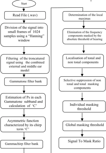
Figure 14. The different steps of the dynamic psychoacoustic model

Figure 15. Change of the dynamic psychoacoustic model from one troncatured wave signal (1024 samples) to another

We used the term ‘dynamic’ because if we move from one toncatured wave signal to another the shape of the Gammachirp filter bank used by the psychoacoustic model will be modified Note:



1024

.



samples

Signal wav

i

: The th

i

( 1 i N) troncatured wave

signal using the Hanning window (1024 points)

1 2 7 2 8 C C C _i    :The th

i

(1 i N) vector containing the 28 chirp

term values. It corresponds to the th

i



1024.



samples Signal w av

i

. Start

Read File (.wav) Division of the signal into

small frames of 1024 samples using a “Hanning”

window

Determination of the local maximas

Localisation of tonal and non tonal components

Selective suppression of non tonal and tonal masking

components

Individual masking threshold

Global masking threshold

Signal To Mask Ratio

Filtering of the troncatured signal using the combined

external and middle ear model

Elimination of the frequency components masked by the absolute threshold of hearing

Gammatone filter bank

Estimation of Ps in each Gammatone subband and

calculation of ‘C’

Gammachirp filter bank

Asymmetric function characterized by its chirp

term ‘C’









¨ 1 1 . . . 8 1024 27 ( 28 27 14 28 28 ) 1 . . . 1024 27 ( 28 2 _{28 2} ) 2 1 1 ₁ 1 1 C SMR Signal wav GFB P A M Step C SMR samples _{C SMR} Sub Step bands C Signal wav GFB P A M Step C samples C _Sub bands   _{ }   _{ }   _{ }     _{ }        _{  } _{ } _{ } _{ }  _{ }_                  





¨ 1 8 27 14 _{28 2} ¨ 1 1 . . . 8 1024 27 ( 28 27 14 28 28 ) 2 SMR SMR SMR Step C SMR Signal wav GFB P A M Step C SMR samples _{N C SMR} Sub Step N bands _N N   _{ }   _{ }   _{ }  _{  } _{ } _{ } _{  } _{ } _{ } _{ }         _{ }   _{ }   _{ }     _{ }       _{  } _ _{ } _                N                                _  _  _  

( 28 ) Su b ba n ds

G F B

i

: The th

i

(1 i N) Gammachirp filter bank (28

subbands) corresponding to the th

i



1024

.



samples

Signal wav

i

8 14

. .

Step Step

P A M

i

        





















: The Psychoacoustic Model as shown in Figure

14, corresponding to the th

i



1 0 2 4



. s a m p l e s S i g n a l w a v i and beginning from step 8 (Determination of the local maximas) to step 14 (Signal To Mask Ratio)

1 2 7 2 8 ¨ S M R S M R S M R _i                        :The th

i

(1 i N ) vector containing the 28

SMR values. It corresponds to the th

i



1 02 4

.



sa m p le s

S ig n a l w a v

i

V. EVALUATION OF SOUND COMPRESSION RATIO The compression ratio CR is defined by the following expression:

_ _

_ _

size wav signal CR

size compressed signal

 (14)

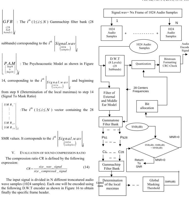
The input signal is divided in N different troncatured audio wave samples (1024 samples). Each one will be encoded using the following D.W.T encoder as shown in Figure 16 to obtain finally the specific frame header.

Figure 16. The detail architecture of the D.W.T encoder

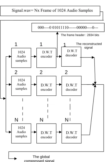
The N all header frames will be decoded using the decoder block system as shown in Figure 17 to obtain finally our compressed signal. D.W.T (8 Levels) (28 Subbands) Quantization Bitstream Formatting CRC-Check Filter of External and Middle Ear Model Gammatone Filter Bank Ps1 Ps28 C1 C28 Gammachirp Filter Bank Determination of the local maximas Global Masking Thershold SMR(dB) SNR(dB) -SMR(dB) = MNR(dB) Return To SNR MNR<0 SNR(dB) MNR>0 Bit allocation

Signal.wav= Nx Frame of 1024 Audio Samples

1024 Audio Samples 1 1024 Audio Samples N + - - - - - - + 1024 Audio Samples 28 Centers Frequencies Audio Encoded Signal Side information Coded data

Figure 17. The D.W.T decoder

Figure 18. The D.W.T encoder and decoder

In order to evaluate the proposed codec using the D.W.T and the dynamic Gammachirp psychoacoustic model, we used for various bitrates some types of sound such as Slow, Soul and Rock. The evaluation is based on the compression ratio defined as the quotient between the size of the original file and the compressed file. Table 2 contains the types of the sound

files used for the test, their capacities, their durations and the compression ratios calculated for each bitrate.

TABLE II. D.W.T COMPRESSION RATIO VALUES USING A BITRATE OF

96KBITS/S,128KBITS/S AND 160 KBITS/S

Signal. wav Duration (s) Capacity (Ko) 96 Kbit/s 128 Kbits/s 160 Kbits/s Slow 28 2426 12.578 10.661 8.239 Soul 22 1910 12.629 10.734 8.481 Rock 20 1680 12.893 10.954 8.612 Jazz 25 2166 12.735 10.824 8.569

The weakest compression ratio is given for the flow of 160 Kbits/s and the highest is given for the flow of 64 Kbits/s. However, the weaker the bitrate, the higher the compression ratio is and the less intelligible its quality becomes. Based on the results obtained in Table 2, the proposed encoder using the D.W.T repartition (28 subbands) and the dynamic Gammachirp filter bank takes account of the masking phenomenon and the critical bands. The second part of our evaluation will focus on comparing the compression ratio obtained from the proposed D.W.T model and the classical MPEG1 one using a bitrate of 128kbits/s which gives the best compromise between compression ratio and sound quality [4]. TABLE III. COMPARISON BETWEEN THE CLASSICAL MPEG1 ENCODER

AND THE PROPOSED D.W.T ENCODER

The classical MPEG1 encoder

The proposed D.W.T encoder

Number of subbands 32 28

Number of samples per subband

32 (for each subband)

Between : 4 and 128 (as shown in Table 1) Size of the troncatured

signal 1024 samples 1024 samples Psycho- Acoustic model Classical Psychoacoustic model Psychoacoustic Model using an external and middle

ear model and a dynamic Gammachirp

filter bank

Table 4 contains the type of the sound files used for the test, the compression ratio values using the classical MPEG1 codec and the proposed D.W.T one

TABLE IV. THE SOUND COMPRESSION RATIO COMPARISON USING THE CLASSICAL MPEG1 ENCODER AND THE PROPOSED D.W.T ENCODER

(BITRATE:128KBITS/S)

Signal.wav The classical MPEG1 codec The proposed D.W.T codec Slow 7.393 10.661 Soul 7.614 10.734 Slow 7.393 10.661

The Table 4 reveals that sound compression using D.W.T is the best one. In fact, its average compression ratio presents an improvement of 42.23% in comparison to the classical Signal.wav= Nx Frame of 1024 Audio Samples

1024 Audio samples D.W.T encoder D.W.T decoder 1024 Audio samples D.W.T encoder D.W.T decoder 1024 Audio samples D.W.T encoder D.W.T decoder The global compressed signal

1

2

N

1

1

2 2

N N

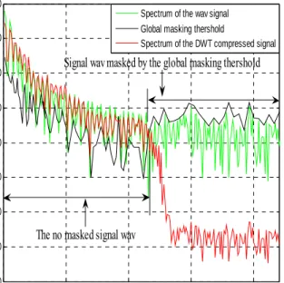
000----0 01011110---00000----0---The frame header : 2834 bits Bit Unpacking Decode Wavelet Coefficients Inverse Wavelet Transform Bit allocation Reconstructed Output Wavelet Coefficients The reconstructed signal

MPEG1 coder. The spectrum of original and compressed signal using the D.W.T and the classical MPEG1 model are shown in Figures 19 and 20.

0 5000 10000 15000 20000 -10 0 10 20 30 40 50 60 70 Frequency(Hz) A m pl it ud e (dB )

Spectrum of the wav signal Global masking thershold

Spectrum of the DWT compressed signal

Signal wav masked by the global masking thershold

The no masked signal wav

Figure 19. Spectrum of the original and the compressed signal using the D.W.T model 0 5000 10000 15000 20000 0 10 20 30 40 50 60 70 Frequency(Hz) A m pl it ude( dB )

Spectrum of the wav signal Global Masking Thershold

Spectrum of the classical MPEG1 compressed signal

The masked signal wav by the global masking thershold

The no masked signal wav

Figure 20. Spectrum of the original and the compressed signal using the classical MPEG1 model

The compressed signal is the mask effect of the global masking threshold on the original audio file spectrum. Concerning the D.W.T model, we note that the global masking thershold masked the spectrum of the original wave signal from 11700Hz. This action introduces a degradation and

inaudibility for all frequencies superior to this frequency (11700Hz). All those frequencies are inaudible since theirs amplitudes are below the absolute threshold of hearing. In our view, the D.W.T model is better in comparison to the classical MPEG1 one. In fact, if we compare the spectrum of the two compressed signals appearing in Figures 19 and 20 we remark that the frequency degradation begins at 16500Hz concerning the classical MPEG1 model and 11700Hz for the D.W.T model. We remark also that D.W.T frequencies degradation is more important. So the average of all D.W.T frequencies amplitude is about 1dB whereas it is 11dB for the classical model

VI. AUDIO TEST QUALITY A. Evaluation Using the MUSHRA Listening Test

Subjective assessment of sound quality is the best way to evaluate encoders performance. As a result of a heavy compression, we always have to expect some kind of impairment. The main objective of every compression algorithm is to make this impairment as much pleasant for a human ear as possible. There are several known methods used for subjective assessment of audio codecs quality. For this purpose we used the EBU MUSHRA method, the most suitable for testing compressed audio samples with a very low bitrates.

MUSHRA stands for MUltiple Stimulus with Hidden Reference and Anchors [5] and is a methodology for subjective evaluation of audio quality, to evaluate the perceived quality of the output from lossy audio compression algorithms. It is defined by ITU-R recommendation BS.1534-1 [5]. The MUSHRA test method is the result of 6 years work by many people [6]. It was devised to meet a need for a subjective test method that was appropriate to intermediate audio quality systems. It is used in tests that are repeatable and reproducible. The fundamental characteristics are: 1. multiple stimuli being offered to the subject; 2. one of the stimuli is a known reference; 3. one of the stimuli is a hidden reference; 4. other stimuli must include hidden anchors with clearly defined parameters. The test method has been used by several different laboratories and is proving to be very effective. In the Mushra test the listener is presented with several audio stimuli for which the listener must give a score between 0 and 100 depending upon their opinion of the quality. The scale has five ranges : “excellent” (100-80), “good” (80-60), “fair” (60-40), “poor” (40-20) and “bad” (20-0) [16].

Figure 21. The grading scale for the MUSHRA listening test.

The selection of compression formats and their specific encoders is a key part of the test preparation phase. Due to extreme time consumption for this type of tests, we decided to compare the proposed audio D.W.T format with only three most widespread audio formats- OGG, AAC and WMA. We

picked the following particular encoders: The proposed D.W.T encoder

AAC encoder included in Apple iTunes 7.0.1 WM Encoder using WMA 9.1 codec

OggEnc 1.0.2 (part of VorbisTools 1.1.1) In order to do a good test, it is important to choose the test

audio signals with some critical elements (such as percussion) to be sure that assessors will be able to even identify the compressed sample. To keep a reasonable length of an entire test session, we decided to pick only four musical samples. Here is a brief list of chosen music sequences defined in the following Table 5:

TABLE V. THE MUSHRA TEST SEQUENCES

Sequence Type Artist Sound Duration (s) Sequence1 Soul _Wonder Stevie Living For _{The City} 30 Sequence2 Slow _Houston Witney A song _{for you} 25 Sequence3 Rock Kevin Barker Worth it 20 Sequence4 Jazz Maurice _Brown Time Tick _Tock 25

This test was intended for comparison of codecs on low bitrates. Our choice was 32 Kbits/s and 64 Kbits/s. The main goal of this experiment was to compare sound quality of the proposed D.W.T audio codec with other widely used audio codecs on very low bitrates. Those codec are already mentioned above. Twenty persons took part in this subjective test. Listeners were mostly between 15 and 25. So they likely still have a good hearing. Seven of them had a previous experience with similar listening tests.

0 20 40 60 80 100

DWT AAC WMA OGG

CODEC M U SHR A SC OR E 32Kbits/s 64Kbits/s

Figure 22. The MUSHRA listening test (Sequence 1)

0 20 40 60 80 100

DWT AAC WMA OGG

CODEC

MU

SHRA SCORE

32Kbits/s 64Kbits/s

Figure 23. The MUSHRA listening test (Sequence 2).

0 20 40 60 80 100

DWT AAC WMA OGG

CODEC MU SH R A SC O R E 32Kbits/s 64Kbits/s

Figure 24. The MUSHRA listening test (Sequence 3)

0 20 40 60 80 100

DWT AAC WMA OGG

CODEC M U SH R A SC O R E 32Kbits/s 64Kbits/s

Figure 25. The MUSHRA listening test (Sequence 4)

100 80 60 40 20 0 Excellent Good Fair Poor Bad

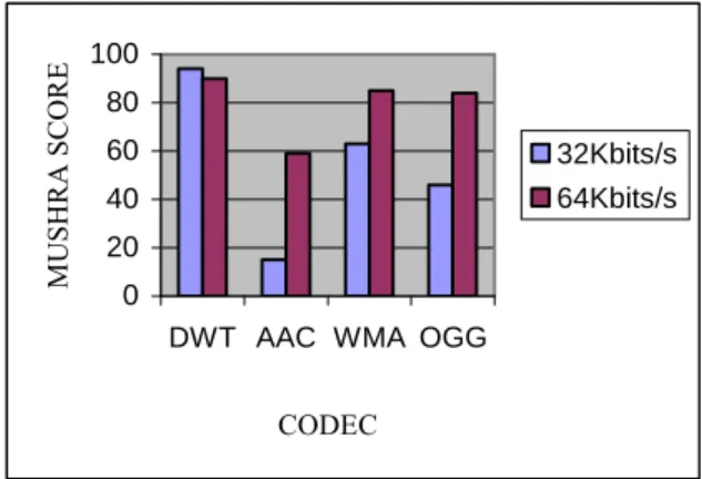
The test results for each sequence are displayed separately in Figures 22, 23, 24 and 25. As for the 32 Kbits/s bitrate, the proposed D.W.T model is the best assessed codec over all sequences. As for the 64 Kbits/s bitrate, the results are much more balanced and the D.W.T model is not always the best. Figure 26 is a numerical representation of overall test results. On bitrate 64 kbits/s, there are no significant quality differences. The quality of most codecs was evaluated as "Good". Only AAC was rated as "Fair". A different situations are on the 32 Kbits/s bitrate. Quality of Ogg and AAC fell down almost to "Poor", in the case of WMA to "Fair". It is very interesting that D.W.T model has a higher rating on bit- rate 32 Kbits/s than on 64 Kbits/s. It may be because the quality of other samples in comparison with D.W.T model was so poor that listeners were much more generous while giving "marks". 0 20 40 60 80 100

DWT AAC WMA OGG

CODEC M U SH R A SC O R E 32Kbits/s 64Kbits/s

Figure 26. The global MUSHRA listening test

Figure 26 is a graphical representation of overall test results. As mentioned above, the D.W.T model is a good choice when the finest sound quality at the very low bitrates is required.

B. SNR Evaluation of The proposed CODEC

The second part of our sound quality evaluation consists in measuring the SNR corresponding to the proposed D.W.T codec which is given by the following equation [12]:

2 2 ( ) 10.log( ) ( ) X Y S SNR S  (15) Where

S

_Xis the mean square of the speech signal and

S

_Y is the mean square difference between the original and reconstructed signal. For this, we select 5 mono wave signals at 705.6kbits/s. Each one is inputed to the proposed D.W.T codec. Next we play the 5 D.W.T audio decoded signals which are compared to the audio signals decoded by the AAC, WMA and Ogg/Vorbis software decoder using the 64kbits/s bitrate. It is widely accepted that SNR cannot truly represent audio quality under perceptual codec and our results confirm this assumption. The SNR results are displayed in the following Figure 27. 0 5 10 15 20 25 30 35 SNR(dB)

Sunset Bolean Rasta Sunny The flight

SOUND

DWT AAC WMA OGG

Figure 27. :SNR Evaluation of the proposed D.W.T CODEC in comparison to

other schemes

VII. ELECTRONIC IMPLEMENTATION OF THE PROPOSED

D.W.TCODEC

A. EvalHardware Description of The D.W.T CODEC The block diagram of the D.W.T codec is represented in the following Figure 28:

Figure 28. Block diagram of the proposed D.W.T codec

The D.W.T CODEC is very flexible encoder and decoder card. It utilizes high speed digital signal processing for real time D.W.T encoding or decoding of analog audio signals. Half duplex functionality permits for the same channel card to be configured to either encode or decode. Incorporation of the D.W.T encoding decoding algorithm results in digital compression of audio signals that reduces the required digital bandwidth to less than half of that required for conventional 64 Kbits/s PCM [15] digitization techniques. As shown in Figure 28, the D.W.T CODEC consists of an embedded RISC/DSP processor, a number of modules that comprise the encoder, a number of modules that comprise the decoder, and a number of I/O modules.

As an audio encoder, it compresses audio data using a proprietary patent-pending motion estimation and rate control algorithm that has been optimized for low latency, fast scene detection and smooth bitrate allocation. The embedded RISC/DSP processor packetizes the compressed data into an output stream format selected by the user. The D.W.T Codec accepts two channels of

I S

2 audio, and uses the audio encoder unctions in the RISC/DSP to generate compressed audio data, which may be multiplexed into the output D.W.T audio compressed stream.

As an audio decoder, the D.W.T CODEC demultiplexes the audio bitstream into its audio and user data components and decompresses the audio information. The output audio is available in

I S

2 or S/P-DIF digital audio format. The D.W.T

CODEC includes a power management module (PMU) and a number of I/O interface modules such as Host/PCI interface (for an external processor, storage and other devices), ROM interface (for boot and other microcode) , General purpose input / output (GPIO), and Phase-locked loops (audio PLL). Two dedicated high-speed SDRAM buses connect the RISC to the two SDRAM interfaces. The encoder SDRAM bus is 32 bits wide, and the decoder SDRAM bus is 64 bits wide. Both interfaces to the external SDRAM devices are 32 bits wide. All modules in the encoder exchange data among themselves via the encoder SDRAM bus. All modules in the decoder exchange data among themselves via the decoder SDRAM bus. The audio encoder core retrieves this data from SDRAM as needed. The audio encoding core reads and writes to the SDRAM the intermediate and final results of the D.W.T encoding process. This compressed data is available to the multiplexer in the RISC via the SDRAM. The audio input unit sends its input data to the RISC via the encoder SDRAM. Audio compression is done by the audio digital signal processing (DSP) extensions in the RISC. The DSP puts the compressed audio back into SDRAM so the data will be available to the multiplexer in the RISC.

B. Audio Compression and Coding

Decoding functions have lower resource requirements. To reach preliminary results as soon as possible, we have implemented all the source program in language C after transformation from Matlab to C with mcc command. The

RISC DSP Decoder Memory Interface Encoder Memory Interface SDRAM 4 M Byte SDRAM 4 M Byte DEMUX MUX D.W.T Decoder Core D.W.T Encoder Core Audio Input I²S Host/PCI Interface External Host PCI Device Bitstream Input Audio Output I²S S/P -DIF

GPIO IDC PMU

ROM Interface

PLL

CLK OSC

final C code has 10478 lines, and occupies 764Kbytes of memory, including input/output libraries from the emulation system. This code is tested into a PC-based prototyping board TMS320C54x DSK

Alternative simulations on fixed point TMS320C5416 DSP have been tried with very few success due to the length of simulation time required for the audio D.W.T compression. The choice of this DSP is due to the high performance required for the application. This DSP contains 8 functional units including two multipliers and two adders. We have measured on different pieces of compiled code (.asm files) the number of instructions that contain concurrent execution of functional units. Table 6 shows the number of instructions with concurrent execution upon the number of concurrent units. The first column designs the compiled file (.asm file) tested. Under column #Instr, the total number of instructions executed for each compiled file is found. Each following column

TABLE VI. NUMBER OF INSTRUCTIONS USING CONCURENT FUNCTIONAL

UNITS

Fle. asm #instr 2C 3C 4C 5C 6C

PAM 5874 486 82 26 10 1 Main 362 10 2 1 D.W.T-Enc 4920 342 74 54 24 8 D.W.T-Dec 3620 88 64 54 24 8 D.W.T 1820 158 76 28 16 8 FFT 4372 196 54 32 7 1 Frame Header 5530 64 14 8 3 2 Quantize 1741 122 18 14 10 4

Note: PAM is the abbreviation of the psychoacoustic model

VIII. CONCLUSION

The demand for compression technology increases every year in parallel with the increase in aggregate bandwidth for the transmission of audio signals. A simple audio encoder scheme based on the Discrete Wavelet Transform and a dynamic Gammachirp psychoacoustic model is presented in this paper. D.W.T usage allows frequency dependant resolution in psychoacoustic model and frequency dependant windowing for quantisation. Masking effects may be better involved by such procedure and artefacts like pre-echo may be suppressed. Our D.W.T encoder was tested using the MUSHRA test sound and compared with other codecs using differents bitrates. This model can achieve transparent quality at bitrate 64Kbits/s and 32Kbits/s in real time for the monophonic CD quality audio signals.

We currently implement the codec in hardware. The Electronic D.W.T codec card corresponding to the Figure 28 is shown in Figure 29. The result should confirm its real−time performance and all other claims made here. We are also working towards lower bitrate (64kbits/s) discrete wavelet

transform audio codec that would gain more momentum because it can match the current PCM bitrate at much better audio quality. A high selectivity was noticed and can lead to some interesting perspectives on audio coding using this type of model.

Figure 29. Electronic card of the D.W.T codec

REFERENCES

[1] ISO/IEC 11172-3 (F), “Information technology - Coding of moving

picture and associated audio for digital storage media at up to about 1.5Mbits/s Part3 : Audio,” 1999

[2] T. Irino and R. D. Paterson, “A compressive gammachirp auditory filter for both physioligical and psychophysical data,” J. Acoust. Soc. Amer. 2001, pp. 2008-2022

[3] B.C.Moore, “An Introduction of the Psychology of Hearing,” 5th ed.

Oxford, UK: Academic, 2003.

[4] G. Davidson, L. Fielder, and M. Antill, “High Quality audio transform

coding at 128Kbits/s,” Proc. IEEE ICASSP, vol.. 2, 1990, pp. 1117-1120

[5] ITU, ITU- R BS 1534. “Method for subjective assessment of

intermediate quality level of coding systems,” 2001

[6] G. Stoll and F. Kozamernik, “EBU Listening tests on internet audio

codecs,” in EBU Technical Review, No.28, 2000

[7] E. Zwicker and H. Fastl, “Psychoacoustics. Facts and Models,”

Springers- Verlag, Berlin, Germany, 2nd Edition, 1999

[8] S.Mallat, “A Wavelet Tour of Signal Processing,” Academic Press, San

Diego, Calif, USA, 2nd edition, 2001.

[9] ISO/IEC JTC1/SC29/WG11 (MPEG), “Generic Coding of Moving

Pictures and Associated Audio: Advanced Audio Coding,” International Standard ISO/IEC IS 13818-7, 1997.

[10] J. O. Smith III and J.S. Abel, “Bark and ERB bilinear transforms,” IEEE Tran. On speech and Audio Processing, Vol. 7, No. 6, November 1999.

[11] C. Wang and Y. C. Tong, “An improved critical-band transform

processor for speech applications,” Circuits and Systems, May 2004, pp 461–464.

[12] A.M.M.A. Najih, A.R. Ramli, A. Ibrahim, and A.R. Syed, “Comparing

speech compression using wavelets with other speech compression schemes,” Student Conference on Research and Development (SCOReD 2003), Aug 2003, pp 55 – 58

[13] K. Ouni, Contribution to the vocal signal analysis using knowledges on the auditory perception and multiresolution time frequency

representation of the speech signals, PhD Thesis on Electrical Engineering, National Engineering School of Tunis, February 2003.

[14] Z. Hajayej, Etude, mise en oeuvre et évaluation des techniques de

paramétrisation perceptive des signaux de parole. Application à la reconnaissance de la parole par les modèles de Markov cachés, PhD Thesis on Electrical Engineering, National Engineering School of Tunis, October 2009.

[15] T. Painter and A. Spanias, “Perceptuel Coding of Digital Audio,”

Proceeding of the IEEE, Vol. 88, Issue 4, pp. 451-515, Avril 2000

[16] P. Rajmic and J. Vlach, “Real-time Audio Processing Via Segmented

wavelet Transform, ” 10th International Conference on Digital Audio Effect , Bordeaux, France, Sept. 2007

[17] P.R. Deshmukh, “Multi-wavelet Decomposition for Audio

Compression,” IE(I) Journal –ET, Vol 87, July 2006

[18] P. Philippe, F. M. de Saint-Martin, and M. Lever, “Wavelet packet filter banks for low time delay audio coding,” IEEE Trans. on Speech and Audio Processing, Vol. 7, No. 3, pp. 310-322, May 1999.

[19] F. Baumgarte, “A computationally efficient cochlear filter bank for

perceptual audio coding,” ICASSP 2001, Vol 5, pp. 3265 – 3268

[20] H.G. Musmann, “Genesis of the MP3 audio coding standard,” IEEE

Trans. on Consumer Electronics, Vol. 52, pp. 1043 – 1049, Aug. 2006

AUTHORS PROFILE

K. Abid received the B.S. degree in Electrical Engineering from the National School of Engineering of Tunis, (ENIT), Tunisia, in 2005, and the M.S degree in Automatic and Signal Processing in 2006 from the same school. He started preparing his Ph.D. degree in Electrical Engineering in 2007. His research interesets in Audio Compression Using Multiresolution Analysis

K. Ouni receiveda Ph. D. degree in Electrical Engineering from ENIT in 2003. He is teatching in Electrical Engineering Department at ISTMT, Tunisia. He is also a researcher at Signal, Image and Pattern Recognition Laboratory, National Engineering School of Tunis (ENIT) Tunisia. His research concern contribution to the vocal signal analysis using knowledges on the auditory perception and multiresolution time frequency representation of the speech signals

N. Ellouze was born in 19 December, 1945. He received a Ph.D. degree in

1977 at INP (Toulouse- France), and Electronic Engineering Diploma from ENSEEIHT in 1968 University P. Sabatier. in 1978. Pr. Ellouze joined the Electrical Engineering Department at ENIT (Tunisia). In 1990, he became Professor in signal processing, digital signal processing and stochastic process. He was the head of the Electrical Department from 1978 to 1983 and General Manager and President of IRSIT from 1987-1994. He is now Director of Research Laboratory LSTS at ENIT, and is in charge of ATS Master Degree at ENIT. Pr. Ellouze has directed multiple Masters and Thesis and published more than 300 scientific papers in journals and proceedings, in the domain of signal processing, speech processing, biomedical applications, pattern recognition, and man machine communication.