www.kuleuven.be
KU LEUVEN
Computing eigenvalues of normal matrices via
complex symmetric matrices
Micol Ferranti and Raf Vandebril
Micol Ferranti
Department of Computer Science
KU Leuven, Belgium
[email protected]
Raf Vandebril
Department of Computer Science
KU Leuven, Belgium
[email protected]
Abstract
Computing all eigenvalues of a modest size matrix typically proceeds in two phases. In a first phase, the matrix is trans-formed to a suitable condensed matrix format, sharing the eigen-values, and in the second stage the eigenvalues of this condensed matrix are computed. The main purpose of this intermediate matrix is saving valuable computing time. Important subclasses of normal matrices, such as the Hermitian, skew-Hermitian and unitary matrices admit a condensed matrix represented by only O(n) parameters, allowing subsequent low-cost algorithms to compute their eigenvalues. Unfortunately, such a condensed for-mat does not exist for a generic normal for-matrix.
We will show, under modest constraints, that normal matri-ces also admit a memory cheap intermediate matrix of tridiago-nal complex symmetric form. Moreover, we will propose a gen-eral approach for computing the eigenvalues of a normal matrix, exploiting thereby the normal complex symmetric structure. An analysis of the computational cost and numerical experiments with respect to the accuracy of the approach are enclosed. In the second part of the manuscript we will investigate the case of nonsimple singular values and propose a theoretical framework for retrieving the eigenvalues. We will, however, also highlight some numerical difficulties inherent to this approach.
Article information
• Ferranti, Micol; Vandebril, Raf. Computing eigenvalues of normal matrices via complex symmetric matrices, Journal of Computational and Applied Mathematics, volume 259, issue A, pages 281-293, 2013.
• The content of this article is identical to the content of the published paper, but without the final typesetting by the publisher.
• Journal’s homepage:
http://www.journals.elsevier.com/journal-of-computational-and-applied-mathematics/
• Published version: http://dx.doi.org/10.1016/j.cam.2013.08.036
Computing eigenvalues of normal matrices via complex symmetric matrices
I Micol FerrantiDepartment of Computer Science, KU Leuven, Celestijnenlaan 200A, 3000 Leuven, Belgium
Raf Vandebril
Department of Computer Science, KU Leuven, Celestijnenlaan 200A, 3000 Leuven, Belgium
Abstract
Computing all eigenvalues of a modest size matrix typically proceeds in two phases. In the first phase, the matrix is transformed to a suitable condensed matrix format, sharing the eigenvalues, and in the second stage the eigenvalues of this condensed matrix are computed. The main purpose of this intermediate matrix is saving valuable computing time. Important subclasses of normal matrices, such as the Hermitian, skew-Hermitian and unitary matrices admit a condensed matrix represented by onlyO(n) parameters, allowing subsequent low-cost algorithms to compute their eigenvalues. Unfortunately, such a condensed format does not exist for a generic normal matrix.
We will show, under modest constraints, that normal matrices also admit a memory cheap intermediate matrix of tridiagonal complex symmetric form. Moreover, we will propose a general approach for computing the eigenvalues of a normal matrix, exploiting thereby the normal complex symmetric structure. An analysis of the computational cost and numerical experiments with respect to the accuracy of the approach are enclosed. In the second part of the manuscript we will investigate the case of nonsimple singular values and propose a theoretical framework for retrieving the eigenvalues. We will, however, also highlight some numerical difficulties inherent to this approach.
Keywords: normal matrix, complex symmetric, Takagi factorization, unitary similarity, symmetric singular value decomposition, eigenvalue decomposition
1. Introduction
Most of the so-called direct eigenvalue methods are based on a two-step approach. First the original matrix is transformed to a suitable shape takingO(n3) operations, followed by the core method computing the eigenvalues of this
suitable shape, e.g., divide-and-conquer, MRRR,QR-methods [10, 22, 23]. Consider, e.g., theQR-method; starting with an arbitrary unstructured matrix, one first performs a unitary similarity transformation to obtain a Hessenberg matrix inO(n3) operations. Next, successiveQR-steps, which costO(n2) each, are performed until all eigenvalues are
revealed.
For some subclasses of normal matrices, e.g., Hermitian, skew-Hermitian, and unitary matrices, the intermediate matrix shapes admit a low storage costO(n) and, as such, permit the design ofQR-algorithms with linear complexity steps [1, 3, 22]. Unfortunately, for the generic normal matrix class, the intermediate structure is of Hessenberg form, requiringO(n2) storage and resulting in a quadratic cost for eachQR-step. An alternative intermediate condensed form might thus result in significant computational savings. To achieve this goal we propose the use of intermediate complex symmetric matrices that can be constructed using unitary similarities. The problem of determining whether a
IThe research was partially supported by the Research Council KU Leuven, projects OT/11/055 (Spectral Properties of Perturbed Normal
Matrices and their Applications), CoE PFV/10/002 Optimization in Engineering (OPTEC), by the Fund for Scientific Research–Flanders (Belgium) project G034212N (Reestablishing smoothness for matrix manifold optimization via resolution of singularities) and by the Interuniversity Attraction Poles Programme, initiated by the Belgian State, Science Policy Office, Belgian Network DYSCO (Dynamical Systems, Control, and Optimization).
Email addresses:[email protected](Micol Ferranti),[email protected](Raf Vandebril)
square complex matrix is unitarily similar to a complex symmetric one has been intensively studied; see, for instance, [2, 8, 21]. Such a similarity always exists for normal matrices [12, Corollary 4.4.4]. One method to perform the unitary transformation of a normal matrix to complex symmetric form was proposed by Ikramov in [13]. It utilizes the Toeplitz decomposition of the normal matrix and symmetries at the same time the two Hermitian terms.
The aim of this article is to provide an initial theoretical basis on which we can continue to build numerical algo-rithms. Again we rely on the two-step principle: First, the matrix is transformed by a unitary similarity transformation to block matrix form, of which the diagonal blocks are complex symmetric. In the simplest case only one block exists [20], and well-known techniques [4, 24, 25] can be used to compute the symmetric singular value decomposition (SSVD), also called Autonne-Takagi factorization [12, 18], of this complex symmetric matrix. Based on the SSVD one can retrieve the eigenvalue decomposition. When multiple blocks are present, it is possible to use the same tech-niques and diagonalize all blocks at once, obtaining a sparse matrix with all blocks diagonal. After that, a specifically designed version of the Jacobi method for normal matrices [9, 17, 19] is used, in order to annihilate the last nonzero off-diagonal entries. Numerical experiments illustrate the effectiveness of the proposed method. Whenever the num-ber of block exceeds one, it will be shown, however, that severe numerical difficulties can appear. More precisely, many articles and authors rely on the property that an irreducible Hermitian tridiagonal matrix cannot have coinciding eigenvalues. Though theoretically correct, this statement might fail in a numerical setting, with nonnegligible impact on the accuracy of the proposed methods (see Section 6 or the discussion in [23, Section 5.45]).
In this article, the following notation is used:ATrefers to the transpose ofA,Ato the conjugate ofAandAH=AT
denotes the Hermitian conjugate. WithA(i : j, ` : k) the submatrix of a matrixAconsisting of rows iup to and including jand columns`up to and includingkis depicted. Withaiwe refer to thei-th column ofA. A matrix is said
to be symmetric ifA=ATand Hermitian ifA=AH. A matrix is real orthogonal ifAAT =ATA=IandAis real, and unitary ifAAH = AHA =I. We might use the expressions real and complex symmetric to stress that the symmetric matrix is real or possibly complex. The elements of a matrixAare denoted byai j, when taking subblocks out of a
partitioned matrix, we refer to them asAk`. The square root of−1 is denoted byı.
The article is organized in two main parts. One part of the article discusses the easy setting in which the intermedi-ate matrix is of complex symmetric form. The second part of the article presents a theoretical approach to deal with the block form, and discusses possible numerical issues. Section 2 recapitulates some known results on normal matrices, the singular value decomposition and results from [20]. In Section 3, under some constraints, the theoretical setting for eigenvalue computations of normal matrices whose distinct eigenvalues have distinct absolute values is consid-ered. The unitary similarity transformation as well as the link with the SSVD is presented to reveal the eigenvalues. Section 4 supports the theoretical discussion by numerical experiments. In Section 5 the generic nonsingular case is investigated. The similarity transformation will now result in a block structured matrix, which can be diagonalized efficiently. The eigenvalues of this latter sparse block matrix are then computed via a Jacobi-like diagonalization pro-cedure. In Section 6 some numerical experiments and observations with respect to the latter structure are presented. We also compare the performance of our method with that of [13] in relation to different distributions of eigenvalues and singular values: we show that both methods can suffer from discrepancies between their theoretical and practical behavior.
2. Preliminaries
This section highlights some essential properties of normal matrices, the singular value decomposition, and some other results required in the remainder of the text.
A singular value decomposition ofAis a factorization of the formA=UΣVH, whereU,V are unitary matrices, andΣis a diagonal matrix with nonnegative real entriesσ1, . . . , σn, we writeΣ = diag (σ1, . . . , σn). The diagonal
elements ofΣare called the singular values ofAand the columns ofU andV are called the left and right singular vectors respectively. A singular valueσiis said to be a multiple singular value if it appears more than once on the
diagonal ofΣ. A standard choice consists of ordering the singular values such thatσ1 ≥ · · · ≥ σn [10]. We will
implicitly assume that every singular value decomposition in this article has this conventional form, except when stated otherwise, and we will stress this by naming it an unordered singular value decomposition. It is well-known that the singular value decomposition for a matrix withndistinct singular values is essentially unique [10], which signifies unique up to unimodular scaling. The unordered version is also unique up to permutations of the diagonal element as long as the singular values are unique.
Suppose that the matrix has singular values of multiplicities exceeding one, so that uniqueness is lost. One then still has uniqueness of the subspaces associated with equal singular values, as given by the following theorem.
Lemma 1(Autonne’s uniqueness theorem, Theorem 2.6.5 in [12]). Let A ∈ Cn×n and let A = UΣVH = WΣZH be two, possibly distinct, singular value decompositions. Then there exist unitary block diagonal matrices B =
diag(B1,B2, . . . ,Bd)andB˜ =diag( ˜B1,B˜2, . . . ,B˜d), such that U =W B, V =ZB and B˜ i=B˜iwhenever the associated
singular value differs from zero.
In general, given a matrixA∈Cn×nand a singular value decompositionA=UΣVH, we have thatAAH=UΣ2UH
andAHA=VΣ2VHare eigenvalue decompositions ofAAHandAHArespectively, having orthonormal eigenvectors. If
A∈Cn×nis normal, thenAAH=AHA, so the columns ofUandVboth form a basis ofCn, made out of eigenvectors
of the same matrix. This means that all columns ofU and all columns ofV stemming from an identical, possibly multiple, singular value must span the same eigenspace ofAAH.
The existence of an eigenvalue decomposition with orthogonal eigenvectors, is equivalent to being normal.1 So for a normal matrixAhaving an eigenvalue decompositionA=QΛQH, whereΛ = diag (λ1, . . . , λn) andQQH =I,
we can always obtain a singular value decomposition. Simply consider matricesΣ = diag (|λ1|, . . . ,|λn|) andΩ =
diageıθ1, . . . ,eıθn, where λi = |λi|eıθi, for all i = 1, . . . ,n. Then A = QΣ(QΩ)His an unordered singular value
decomposition.
Remark 2. Consider a polar decompositionA=PWofA∈Cn×n, i.e., a factorization wherePis Hermitian positive
semidefinite andW is unitary. LetP=UΣUHbe a unitary2eigenvalue decomposition ofP. ThenA=UΣWHUH
is an unordered singular value decomposition of A. A matrix is normal if and only if its polar factors commute [11]. Hence, If Ais normal, its polar decomposition provides us two possibly different unordered singular value
decompositions:A=UΣWHUH=(WU)ΣUH.
In [20] the following theorem was proved, serving as a basis for the investigations proposed in this article.
Theorem 3(Theorem 1 in [20]). Let A∈Cn×nbe a normal matrix, having distinct singular values and A=U BVH, with U,V unitary and B a real matrix. Then AU=UHAU and AV =VHAV will be symmetric matrices.
The algorithm proposed in [20] relies on the standard bidiagonalization procedure to computeU,V, andB, and it allows the use of a real orthogonal transformation whenAis real. However, as we are going to show in Subsection 3.1, the same result is possible with less strict demands; in particular it is shown that bidiagonal matrixBis not required.
3. Eigenvalue retrieval of normal matrices unitarily similar to a symmetric one
This section proposes an alternative approach, not relying on an intermediate Hessenberg matrix, for computing the eigenvalues of a normal matrix whose distinct eigenvalues have distinct absolute values. The more general setting is presented in Section 5.
3.1. Unitary similarity transform to symmetric form
A construction of a unitary similarity transformation to complex symmetric form was discussed in [20]. In that article the normal matrix was assumed to have distinct singular values. The proof of Theorem 3 was explicitly based on the construction of the complex symmetric matrix and used the intermediate matrixB. However, the matrixBis theoretically redundant, and one can formulate more general versions of Theorem 3.
Lemma 4. Let A∈Cn×nbe a normal matrix. Then AAHis real if and only if A=Qdiag (σ1W1, . . . , σdWd,0n−r)QT,
whereσ1, . . . , σdare the distinct positive singular values of A, r=rank(A), Wiis unitary for each i=1, . . . ,d, and Q
is a real orthogonal matrix.
1There is an extended list of properties equivalent to being normal, see, e.g., [6, 11].
Proof. IfA=Qdiag (σ1W1, . . . , σdWd,0n−r)QT, thenAAHis trivially real. Let us consider the other implication. Let
A=PWbe a polar decomposition ofA. ThenP2 =AAHis real, so alsoPmust be real. Consider a real orthogonal eigenvalue decompositionP=QΣQT. Then
Σ =diag σ1In1, . . . , σdInd,0n−r
,
wherer =rank(A), andni is the multiplicity ofσi. An unordered singular value decomposition of Ais given by
A=QΣQTW, and by Remark 2 alsoA=(W Q)ΣQT is one. By Lemma 1, we find
QTW Q=diag (W1, . . . ,Wd,Wd+1).
ReplacingWbyQdiag (W1, . . . ,Wd,Wd+1)QTin the polar decomposition, we have that
A=QΣdiag (W1, . . . ,Wd,Wd+1)QT =Qdiag (σ1W1, . . . , σdWd,0n−r)QT.
The previous result provides fundamental information showing that, once we require AAHto be real, a normal matrixAis symmetric if and only if everyWi from Lemma 4 is unitary and symmetric. We are now interested in
determining conditions under which this property holds. A first sufficient condition is straightforward.
Corollary 5. Let A∈ Cn×nbe a normal matrix having its positive singular values distinct (multiplicities one), and
suppose AAHis real. Then A is symmetric.
Proof. Write Ain the formA = Qdiag (σ1W1, . . . , σdWd,0n−r)QT. The positive singular values have multiplicity
one, so the unitary matricesWiare of size 1×1 for eachi=1, . . . ,d, implying symmetry.
The previous corollary clearly extends Theorem 3. Indeed, ifBis real, thenAUAHU = BB
His also real, andA U
is symmetric. The same holds forAV. Furthermore Lemma 4, and thus also Corollary 5, are still valid when 0 is a
multiple singular value, no matter how large its multiplicity. Corollary 5 can be generalized even further.
Corollary 6. Let A∈Cn×n be normal and suppose that distinct eigenvalues of A (possible higher multiplicity) have
distinct absolute values. If AAHis real, then A is symmetric.
Proof. WriteAin the formA =Qdiag(σ1W1, . . . , σdWd,0n−r)QT. Each unitary matrixWjhas only one eigenvalue
eıθjwith multiplicityn
j, soWj=eıθjInj for eachj=1, . . . ,d, implying symmetry.
We can now generalize the results of Theorem 3.
Theorem 7. Let A ∈ Cn×n be a normal matrix and A = U BVH, with U,V unitary and B a real matrix. If distinct eigenvalues of A have distinct absolute values, then AU=UHAU and AV =VHAV are symmetric normal matrices.
Proof. BothAUAHU =BBHandAVAHV =BHBare real matrices and their eigenvalues are equal to those ofA. Thus
Corollary 6 holds forAUandAV, implying symmetry.
Example 8. To clarify the meaning of the previous results, we include a practical example. Consider the normal matrix A= "ı I2 −I2 I2 ıI2 # .
The eigenvalues ofAare 0 and 2ı, both with multiplicity 2. Use the reduction proposed in [20] to get the unitary matrixVsuch thatAVAHV is real, whereAV =VHAV. The matrixAVhas the same eigenvalues asA, and they comply
with the hypothesis of Corollary 6. We obtain
V = 1 0 0 0 0 0 ı 0 0 −ı 0 0 0 0 0 1 andAV = ı ı 0 0 ı ı 0 0 0 0 ı ı 0 0 ı ı ,
This result strongly depends on the eigenvalues as required in the hypothesis. It does not need to hold when distinct eigenvalues share the same modulus: see, e.g., Example 13.
However, ifAAH is real, it is always possible to determine ifAis symmetric, even when the distribution of the
eigenvalues is unknown. The following theorem shows a necessary and sufficient condition for the symmetry ofA.
Theorem 9. Let A∈Cn×nbe normal and suppose that AAHis real. Then A is symmetric if and only if AAH=AA.
Proof. ConsiderAin the formA =Qdiag(σ1W1, . . . , σdWd,0n−r)QT from Lemma 4. The matricesWiare unitary;
they are thus symmetric if and only ifWiWi=Ini for eachi=1, . . . ,d. That is equivalent to
AAH=Qdiag(σ21In1, . . . , σ
2
dInd,0n−r)Q
T=AA.
We can reconsider now the sufficient conditions on the eigenvalues required in Corollaries 5, 6, and Theorem 7. As we saw, they ensured the matricesWito be unitary diagonal, trivially implying thatAAH = AA. They are thus
particular cases in which the condition of Theorem 9 is satisfied.
Even though the constraint AAH = AAallows us to treat most of normal matrices, some particular important
subclasses do not possess this property. For instance, it does not hold for generic real orthogonal and unitary non-symmetric matrices, or for nonzero real skew-non-symmetric matrices. The development of a new numerical method for computing eigenvalues implies hence also the capability of dealing with these matrices, which is proposed in Section 5.
3.2. Exploiting the symmetric singular value decomposition to retrieve the eigenvalues
Even if the conditionAAH=AAis sufficient to ensure the symmetry, it does not ensure essentially uniqueness of
the singular value decomposition. In this section we rely on additional constraints in order to exploit the symmetric structure to compute an eigenvalue decomposition ofA. We suppose for now that the normal matrixAunder consider-ation complies with the assumptions in Theorem 7 (distinct eigenvalues have distinct absolute values), the other case is discussed in Section 5. Both the normality and the symmetric structure play an essential role in constructing the new algorithm. Let us consider some decompositions for both normal and symmetric matrices and design an algorithm based on them.
Normal matrices. Suppose thatAis normal, admitting a singular value decompositionA=UΣVH, and an eigenvalue decompositionA=QΛQH. As we showed, with a suitable permutationΠ,ΛΠ = ΣΩ, withΩa unitary diagonal matrix containing the arguments of all eigenvalues andΣcontaining the moduli. In fact we haveA=QΛQH=UΣΩ(VΩ)H. This implies, once we know the singular value decomposition, that under the conditions imposed on the normal matrices, Ω = VHU (see proofs of Corollary 5 and Corollary 6), which can be used to retrieve the eigenvalues. Unfortunately computing both a left and right set of singular vectors is quite expensive.
Symmetric matrices. A complex symmetric matrixAis not normal in general, but always admits a so-called sym-metric singular value decomposition (SSVD), often also named a Takagi or Autonne-Takagi factorization [12, 18]. This factorization has the form: A =WΣWT, whereΣis a diagonal matrix containing the singular values andW is a unitary matrix: WWH = WHW = I. It is clear that this is a special type of singular value decomposition. What makes an SSVD particularly interesting is the fact that complex conjugates of singular vectors are left singular vectors. Thus, only one set of singular vectors should be computed leading to an overall reduction of the computational cost, generally depending on the method used to compute the SSVD (see Section 4.1), and of the storage costs.
Normal and symmetric. If the matrixAis both normal and complex symmetric, we have the possibility to combine the two decompositions. Once we have computed an SSVDA =WΣWT, we can always obtain the eigenvalue de-compositionA=W(ΣΩ)WH, as for the generic normal matrix, but this time computing the moduli of the eigenvalues
is much more attractive. Computing the diagonal matrixΩ = WTW requires only one set of right (or left) singular
vectors.
The entire algorithm for a normal matrix whose distinct eigenvalues have distinct moduli can therefore be sum-marized in three steps:
• Apply a first transformation to obtain a symmetric matrixA, see [20];
• use one of the well-known methods to compute an SSVD factorizationA=WΣWT. There exist several ways to manage this problem, see e.g., [4, 24, 25] and Section 4 where they are briefly discussed;
• compute the diagonal matricesΩ = WTW andΛ = ΣΩ. The factorizationA=WΛWHis then an eigenvalue
decomposition ofA.
4. Numerical experiments
In this section, we first compare the theoretical cost of the proposed method with that of the generic QR algorithm. Thereafter, we present the results of some numerical experiments in order to investigate the accuracy of the algorithm. We implemented our algorithm relying on both the twisted factorization method [25] and the QR-based method [5] to compute the SSVD of a symmetric matrix.3 We observed in some preliminary tests that these two approaches
outperform the divide-and-conquer approach [24] in terms of accuracy.
4.1. Complexity analysis
Both the methods proposed in [5, 25] for computing the SSVD must be applied to symmetric tridiagonal matrices. Hence an additional transformation to symmetric tridiagonal form is required, e.g., by Householder transformations. The overall algorithm for the eigenvalue retrieval consists of four steps:
• CS: transformation of a normal matrixAto normal symmetric formC:A=U1CUH1;
• TRI: transformation of the normal symmetric matrix to (possibly not normal) symmetric tridiagonal form:
C=U2T UT2;
• TF: computation of the SSVD:T =U3ΣUT3;
• ED: retrieval of the eigenvalue decomposition based on the SSVD:A=UΛUH.
Let us consider in detail the costs of the individual steps and compare the resulting complexity with that of the classical QR method. In the following we will always omit lower order terms and consider only the dominant terms. The first step requires 8
3n
3flops for the bidiagonalization, 8n3flops for computingCThe second step requires 4 3n
3
flops for the tridiagonalization and 2n3additional flops for computingU2. The transformation of a normal matrix to
complex symmetric tridiagonal form thus has a total cost of 12n3flops.
The cost of the third step strongly depends on the selected method. The QR-based approach translates the algo-rithm for computing the singular values of a bidiagonal matrix to the tridiagonal setting. As one relies on the QR factorization ofT TH, this results in a double shifted QR-step. This method needsO(n2) flops for computing singular
values andO(n3) flops for computing the singular vectors if all operations are accumulated. On average, the total cost
is 6n3for computing the whole SSVD [16]. Alternatively, the twisted factorization method focuses on computing the
singular vectors, assuming thereby that the singular values are known. This method is based on the MRRR algorithm for computing the eigenvectors of symmetric tridiagonal matrices [5]. It has a total complexity ofO(n2) for comput-ing the whole SSVD [25]. But it must be stressed that this holds only when all scomput-ingular values are well separated. In practice, this method’s accuracy suffers greatly from singular values being too close.
The fourth and last step has also a neglectable cost ofO(n2), and 4n3additional flops are necessary to applyU2
toU3andU1to the obtained product. In conclusion, to compute the entire eigenvalue decomposition, we need 16n3
and 22n3flops, utilizing the twisted factorization or QR-based method respectively. On the other hand, the classic QR method for generic matrices requires in total 25n3for the average case [10].
4.2. Accuracy
In this section we present the results of some practical experiments. We build some normal matrices with evenly distributed singular values (minimal gap equal to 0.05), as we want to compare the performances of the QR based and the twisted factorization methods. Normal matrices with predeterminated eigenvalues were generated as follows: given the vectorλcontaining the eigenvalues, the matrixAis defined asA=Zdiag(λ)ZH, whereZis a random unitary matrix obtained by the QR decomposition of a random complex matrix. For every sizen=50,10, . . . ,1500 the same experiment is repeated three times, and the mean value is taken for every measured magnitude.
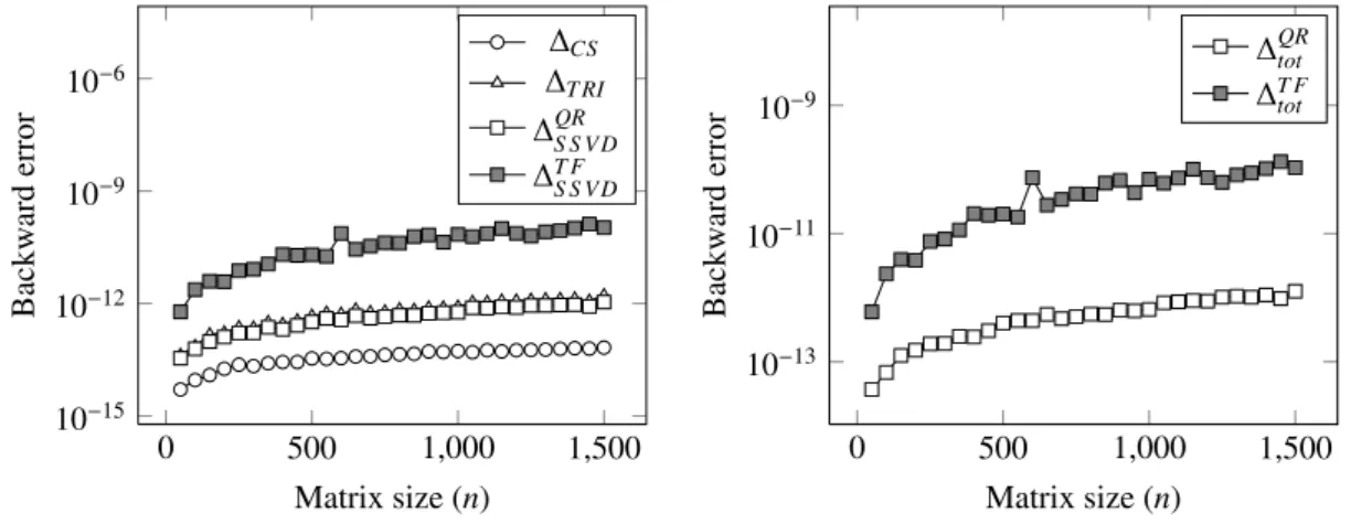
The errors in Figure 1 related to the individual steps were measured as ∆CS = kA−U1CU1Hk kAk , ∆T RI= kC−U2T UT2k kCk , ∆ QR S S V D= kT−UQRΣUQRT k kTk , ∆ T F S S V D= kT −UT FΣUT FT k kTk ,
wherek · kis the two-norm and ”QR” and ”TF” indicate if the singular vectors are obtained via the QR-based or the twisted factorization method respectively.
0 500 1,000 1,500 10−15 10−12 10−9 10−6 Matrix size (n) Backw ard error ∆CS ∆T RI ∆QR S S V D ∆T F S S V D 0 500 1,000 1,500 10−13 10−11 10−9 Matrix size (n) Backw ard error ∆QR tot ∆T F tot
Figure 1: Backward errors of the single steps and of the total decomposition
The total backward error was measured as ∆tot=
kA−U1U2U3ΣU3TU2TU1Hk
kAk ,
withU3varying, depending again on the method selected to perform the third step. These error measures reflect the
accuracy of the entire decomposition, capturing both eigenvalues and eigenvectors. The overall relative eigenvalue errors are then determined as
∆λ= max
i=1,...,n
|λi−λ˜i| |λi|
!
, and∆eig = max
i=1,...,n
|λi−λˆi| |λi|
!
,
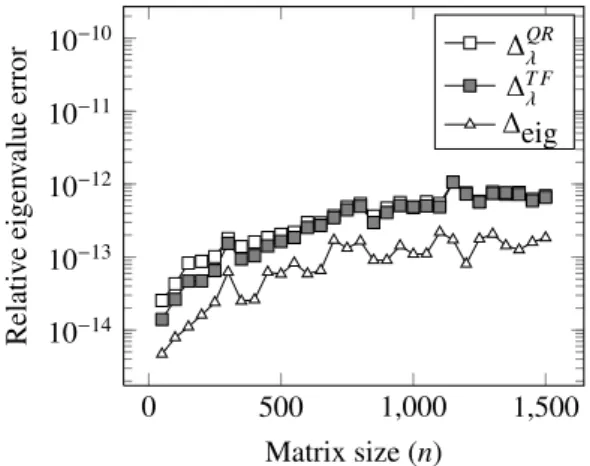
where ˜λiare the computed eigenvalues, and ˆλiare the eigenvalues computed by Matlab’seigcommand. In Figure 2,
we compare different values of∆λ, depending on the method chosen for computing the SSVD, with the corresponding
error∆eig.
5. The generic nonsingular normal case: intermediate block matrices
In the previous section, some constraints were put on the eigenvalues and singular values, to compute the eigen-values of a normal matrix in an alternative manner. It is possible, however, to use similar techniques to compute the eigenvalue decomposition of an arbitrary nonsingular normal matrix. In this section, we will provide a framework, where the original matrix is first transformed to a suitable block form; next, all blocks are diagonalized simultaneously; and, finally, a global eigenvalue decomposition of the matrix is deduced.
0 500 1,000 1,500 10−14 10−13 10−12 10−11 10−10 Matrix size (n) Relati v e eigen v alue error ∆QR λ ∆T F λ ∆eig
Figure 2: Relative eigenvalue errors
5.1. Unitary similarity transformation
Forthcoming Theorem 10 states that the algorithm for reducing a normal matrix to symmetric form always results in a block matrix, whose diagonal blocks are symmetric. The proof is based on a further specialization of the results from Theorem 3 and utilizes explicitly the reduction to bidiagonal form, because theoretically this can ensure the absence of multiple singular values. Suppose namelyBto be a bidiagonal matrix,BHBthen becomes an Hermitian
tridiagonal matrix. It is well-known that an irreducible, i.e., having nonzero off-diagonal elements, Hermitian tridi-agonal matrix must have distinct eigenvalues (see, for example, [10, Theorem 8.5.1] or [23, Section 5.37]). Hence, in the preprocessing step performing the unitary similarity transformation to complex symmetric form, one can easily detect nonsingularity and absence of singular values of a higher multiplicity as one passes via the bidiagonal form.
Furthermore, assume that the nonsingular normal matrixAhas singular valuesσi, having multiplicitiesmi. This
implies that the resulting matrixBhas at leastm=maximi−1 zeros on the superdiagonal. Moreover, in each of the
diagonal blocks, all the singular values must be different from each other.
Theorem 10. Let A∈Cn×nbe a nonsingular normal matrix and assume A=U BVH, with U,V unitary and B a real
bidiagonal matrix. The indices{i1, . . . ,im−1}indicate the rows i` for which the superdiagonal element bi`,i`+1equals
zero (by definition we set i0 =0,and im=n).
Then we have for AU =UHAU and AV =VHAV that the diagonal blocks AU(i`−1+1 :i` , i`−1+1 : i`)and
AV(i`−1+1 :i`, i`−1+1 :i`)are symmetric for`=1, . . . ,m−1.
The proof is based on a suitable partitioning ofAU. To ease the presentation of the proof we introduce a sort of
block Hadamard product.
Definition 11. Assume a matrix partitioned in blocks A = (Ak`)k` withAk` ∈ Cnk×n` and a set of square matrices Υ = {Υk`}k` withΥk` ∈ Cn`×n` are given. The block Hadamard productC = A◦B Υ is defined as the matrixC
partitioned accordingly toAand having blocksCk` =Ak`Υk`.
We remark thatAk` andΥk` need not have the same dimension since all blocks ofΥk` are square. Moreover, in
general it is not even possible to combine the blocks ofΥk`in a matrixΥ.
Proof of Theorem 10. The proof is inspired by the one presented in [20, Theorem 1] and is subdivided in two parts here. First, different eigenvalue decompositions ofAUAUHare derived, followed by an investigation of the connections
between the eigenvectors. Assumem>1, otherwisei1=nso that Theorem 3 applies.
Eigenvalue decompositions of AUAHU. Assume the factorizationB = UHAV is given, with Bbidiagonal,U andV
unitary, and the indicesi`satisfying the assumptions from the theorem. PartitionAUin blocks (AU)k`:
Furthermore letnk=ik−ik−1+1, this means that (AU)k`is of dimensionnk×n`.
The following relations hold for the matrix productAUAUH:
AUAHU =
UHAU UHAHU=UHAAHU=UHAV VHAHU=BBH=T. (1) The matrixBis real nonsingular and bidiagonal implying thatT is a real nonsingular symmetric tridiagonal matrix. The zero superdiagonal elements in the matrixBintroduce zeros in the sub- and superdiagonal ofT (ti`,i`+1 =0 =
ti`+1,i`), making T reducible. The tridiagonal matrix is hence of block diagonal form with diagonal blocks T`` =
T(i`−1+1 :i` , i`−1+1 :i`), where`=1, . . . ,m−1. Due to the ordering of the singular values in the matrixB, the
diagonal blocks ofT have all eigenvalues different from each other. The eigenvalue decomposition of each individual diagonal blockT``is therefore essentially unique. Consider an eigenvalue decomposition ofAU=QΛQH, where the
eigenvalues in the diagonal matrixΛare ordered accordingly to the matrixT. This means that the diagonal elements of|Λ``|2 equal the eigenvalues of the tridiagonal blockT
``. The matrixT`` admits therefore an essentially unique
eigenvalue decomposition of the formT`` =Qˆ``|Λ``|2QˆH``, with ˆQ``real orthogonal. Combining the decompositions
for each blockT``, we get another eigenvalue decomposition of the matrix product AUAHU = Qˆ|Λ|2QˆH, where the
blocks ˆQk`=0 wheneverk,`.
SinceT is realT =T, Equation (1) combined with the eigendecomposition ofAU =QΛQHgives us three different
eigendecompositions of the matrix productAUAHU:
AUAHU = Qˆ|Λ| 2QˆH, (2) AUAHU = Q|Λ| 2QH, (3) AUAHU = T =T =AUATU=Q|Λ| 2QT. (4)
In the original proof of Theorem 3 (see [20], the casei1 = n) all singular values of Awere assumed distinct.
Hence the diagonal of|Λ|2 contained all distinct values and consequently all invariant eigenspaces are of dimension one implying essentially uniqueness of the eigenvectors. This resulted in the fact thatQ=QΩby combining (3) and (4), withΩa unitary diagonal matrix, proving thereby thatAUis symmetric.
Here, in this setting we can have invariant subspaces of higher dimensions belonging to a single eigenvalue from
AUAHU. Since, however, the eigenvalues are ordered in blocks of distinct eigenvalues we know that the column vectors
of the blockQ:,`=Q(:, i`−1+1 :i`) all belong to different invariant subspaces and are hence orthogonal.
Relations between the eigenvectors. To present a unified link between the matrices ˆQ,QandQ, some extra matrices are needed. Construct a binary matrixPwithpi j=1 if|λi|2 =|λj|2, whereΛ =diag(λi), and partition it according to
AU. The fact that the blocks|Λ``|have all eigenvalues distinct imposes extra structure on the matrixP. All diagonal
blocksP``∈ Rn`×n` are square identity matrices, the matricesP
k` ∈Rnk×n` have at most one nonzero entry (equal to 1) in each row and column. One can see this as a combination of a permutation followed by real diagonal projection matrix containing ones or zeros on its diagonal. The matrixPk`provides, in fact, links between identical eigenvalues
of the diagonal blocks ofAUAHU. Moreover, the matrixPis symmetricPk`=PT`k.
TakingPk`PTk` =Pk`P`kandP`kPT`k =P`kPk`, we see that we get diagonal projection matrices (having either one
or zero on the diagonal) of dimensionsnk×nkandn`×n`respectively. An important relation is the following:
Pk jPj`=Pk`(P`jPT`j), (5)
in words this means: Pk j links the eigenvalues of block|Λkk|to the ones of|Λj j|, this is followed by a link to the
eigenvalues of the block|Λ``|. Hence, we have a link between the block|Λkk|and the block|Λ``|, which is given by
Pk`. Unfortunately, during this transition some links might get lost and this is modeled by the projection operator
(P`jPT`j) retaining only the relations inPk`which are also present inP`j.
Based on (2) and (3) we know that the eigenvectors ˆQandQmust be linked. To obtain the eigenvectors inQfrom the ones in ˆQ, only restricted combinations of columns of ˆQare allowed. Only the eigenvectors belonging to identical eigenvalues and hence to the same invariant subspace can be combined. Using the block Hadamard product and the matrixP, we can write this asQ = Qˆ(P◦BΩ), whereΩis a set of diagonal matricesΩ`k. This product indicates
eigenvalues (imposed byP) of the columns of ˆQ, such to obtain the eigenvectors ofQ. The matrix (P◦BΩ) is unitary
and partitioned according toAU. We remark that the diagonal matricesΩ`kcan be singular. Using (2) and (3) we also
get the following relation: Q=Qˆ(P◦BΩ)=Qˆ(P◦BΩ). Combining (3) and (4) gives usQ= Q(P◦BΥ), withΥ again a set of diagonal matrices. One can also verify that (P◦BΥ) is symmetric, sinceI=QTQ¯=QTQ(P◦
BΥ).
Since the matrix ˆQis block diagonal we obtain the following equations:
Q`k = m X i=1 ˆ Q`i(P◦BΩ)ik=Qˆ``(P◦BΩ)`k=Qˆ``P`kΩ`k (6) Q`k = Qˆ``P`kΩ`k. (7)
This means in fact that the columns ofQ`kandQ`kare reordered and scaled columns of the matrix ˆQ``. Since there
exists a diagonal matrixΓ`ksuch thatΩ`k= Ω`kΓ`kwe get thatQ`k=Q`kΓ`kwhich is in factQ=Q◦BΓ. Equations (6)
and (7) indicate that each block Q`k andQ`kcan be reconstructed by reshuffling and scaling the columns of ˆQ``.
The converse statement is less powerful: some (perhaps none ifQ`k = 0) columns of ˆQ``can be reconstructed by
reshuffling and rescaling some columns ofQ`k. A similar statement holds between the columns ofQ`iandQ`j, we
have forQ`j=Qˆ``P`jΩ`jthatQ`jPji=Qˆ``P`jΩ`jPji. SinceΩ`jis a diagonal matrix of dimensionnj×nj, there exists
another diagonal matrix ˆΩ`iof dimensionni×nisuch thatΩ`jPji=PjiΩˆ`i. Using (5) leads to:
Q`jPji = Qˆ``P`jPjiΩˆ`i=Qˆ``P`i(Pi jPTi j) ˆΩ`i=Q`i(Pi jPTi j) ˆΩ`i.
This means that some of the columns ofQ`jare a scalar multiple of columns ofQ`i.
We now have everything to complete the proof. The``diagonal block of the matrixAUis of the following form:
(AU)``=Q`,:ΛQH`,:=Q`,:ΛQ`,: T =Q`,:Λ Q`,:(P◦BΥ)T =Q`,:Λ(P◦BΥ)QT`,:= m X i=1 m X j=1 Q`iΛiiPi jΥi jQT`j.
Instead of proving that the global sum is symmetric, we can even prove that each of the above terms will be symmetric. Wheni= j, we get:Q`iΛiiPiiΥiiQT`i, which is clearly symmetric (Piiis diagonal). Consider nowi, j, then we have a
term of the formQ`iΛiiPi jΥi jQT`j. Again we use the existence of a ˆΥi jsuch thatPi jΥi j =Υˆi jPi jto obtain the following:
Q`iΛiiPi jΥi jQT`j = Q`iΛiiΥˆi jPi jQT`j = Q`iΛiiΥˆi j Q`jPji T = Q`iΛiiΥˆi j Q`i(Pi jPTi j) ˆΩ`i T =Q`iΛiiΥˆi jΩˆ`i(Pi jPTi j)Q T `i.
This term is clearly symmetric and hence also the complete sum (AU)``will be symmetric.
The proof presented here, relies strongly on the existence of a block diagonal eigenvalue decomposition of the matrixT, which one can assume to exist because we pass via the bidiagonalization procedure. It is therefore unknown yet, whether a general formalism as in Section 3.1 also holds in this case.
Question 12. LetA∈Cn×nbe nonsingular normal. WheneverAAHis real, willAbe a block matrix whose diagonal
blocks are symmetric?
At least we know that the answer is affirmative in specific cases.
Example 13. Suppose thatA ∈R2n×2n is a nonsingular skew-symmetric matrix. Consider the real orthogonal
sim-ilarity transformation from Theorem 3, to obtainC =UTAU. The skew-symmetry implies that all the eigenvalues
are purely imaginary, appearing in conjugate pairs, andAAH =AAT
,A2 =AA. Thus in this case the condition in
Theorem 9 does not hold. We know, however, thatC =(Ci j)i jis a 2×2 block matrix, for which the diagonal blocks
The real orthogonal transformation preserves the skew-symmetry, henceCiiT = Cii = −Cii for bothi = 1,2,
implyingC11andC22to be zero. On the other hand,C21=−C12T. ThereforeCis of the form
C=UTAU= " 0 C12 −CT12 0 # ,
with only the diagonal blocks respecting the symmetric structure.
Example 14. LetU ∈ Cn×n be a unitary nonsymmetric matrix. ThusUUH
, UU butUUH = I is real. All the
singular values ofUare equal to 1. The diagonal blocks under consideration have then size 1×1, being thus trivially symmetric.
5.2. Simultaneous block diagonalization
If the matrix has multiple singular values related to distinct eigenvalues, we cannot directly apply the algorithm described in Section 3, because only the diagonal blocks have the symmetric structure we need. On the other hand, it is possible to apply another transformation to reduce this block matrix to a sparse and handier form.
Theorem 15. Let A∈Cn×nbe a nonsingular normal matrix. Let A=U BVHwhere B is real bidiagonal and U,V are
unitary. Consider the matrix C=UHAU or C =VHAV. Then, there exists a real orthogonal block diagonal matrix
Q=diag(Q1, . . . ,Qm),such that Qi∈Cni×ni for each i=1, . . . ,m and QTCQ has the same block structure as C, with
every block of diagonal or permuted diagonal form.
Proof. Though the proof follows almost directly when considering a decent ordering of the diagonal blocks and singular values, combined with (6), we also provide a slightly different way of looking at the problem, closer to the proofs in Section 3.1.
Assume thatm > 1, otherwise the statement holds trivially. LetB = QΣZT be a singular value decomposition
ofB. Because of the structure ofB, bothQandZcan be taken real orthogonal and block diagonal. If, for instance,
C = UHAU, thenC = QΣ(QTW) is a singular value decomposition of C. Similar reasoning as in the proofs of Corollary 5 and Corollary 6 implies that QTCQ is in the required form, with every block diagonal or permuted diagonal.
The previous result ensures that it is always possible to apply a transformation by a real orthogonal block diagonal matrix, to transform all the blocks of the original matrix to permuted diagonal form at once. If the diagonal blocks ofB
are maximal, meaning that each of them has the maximum possible number of distinct singular values of the original matrix, than we can garantee diagonal blocks. In any case, the resulting matrix has a limited number of nonzero entries, placed in symmetric positions, yielding a significant reduction in the cost of the forthcoming diagonalization. On the other hand, computing the matrixQexplicitly would be too expensive. One more attractive way to get the same result is exploiting the Takagi factorizations of the diagonal symmetric blocks ofA(in case these factorizations are essentially unique), or by considering eigenvalue decompositions of the diagonal blocks of the matrixT in (4).
5.3. From block diagonal to diagonal form
It remains to bring the block matrix to diagonal form. In this section we focus on how to achieve this. We start by considering a block matrix with all the blocks in permuted diagonal form, and we show how to apply the classic Jacobi method for normal matrices, for a fast and accurate diagonalization.
In the literature there are many examples and variants of this classic method, whose oldest and simplest version was presented by Jacobi in 1846 [14]. The main idea for computing the eigenvalues of a symmetric matrix, consists of minimizing at every stage the sum of the squares of the off-diagonal elements. This is accomplished by a rotation, acting on a selected off-diagonal entry called pivot. The main differences between the various Jacobi methods are about the class of matrices they are able to deal with, and the strategy used to choose pivots. The most general instance is due to Goldstine and Horwitz [9], and allow us to work with every normal matrix. Given a generic normal matrixA∈Cn×n, one single step of the iteration can be summarized as follows:
• compute ω=aj j+akk 2 , and θ= 1 2 arg −det " aj j−ω ajk ak j akk−ω #! ;
• findφandαsuch that
γ=e−ıθajk+eıθak j, φ= 1 2 arctan |γ| ree−ıθ aj j−akk , and α= arg (γ) ;
• perform the unitary similarity transformation A = GHAG,where the nontrivial part ofG different from the
identity is located in positions (j,k),(j,j),(k,j),and (k,k). Written as a 2×2 matrix, it equals
Gjk=
"
cosφ −eıαsinφ
e−ıαsinφ cosφ #
and acts on the j-th andk-th rows and columns ofA.
Typically the Jacobi method is considered to be slow. In our setting, however, it serves as an adequate algorithm for zeroing the remaining off-diagonal elements. There are two big advantages. The rate of convergence of the Jacobi method is quadratic with respect to the number of entries that must be annihilated [15]. That is, in case of a dense matrix, proportional toN = n(n2−1), making the algorithm not suitable for large matrices. The situation is, however, different in our case, where the matrix has a limited number of nonzero off-diagonal entries: when all the blocks have, for instance, the same size n
k, the number of entries to annihilate is proportional toN = n(k−1)
2 , resulting in a faster
algorithm. This is not the only benefit: the entries that we want to eliminate follow a particular pattern, positioned on the permuted diagonals of a block matrix. As a result it is not necessary anymore to scan the entire matrix to select the pivot: when one nonzero element is found in a certain block, one does not need scan the rest of the row and column. Moreover, nonzeros entries appear in symmetric position, so it is necessary to know only n(n2+1) entries to figure out their whole distribution. In addition, the transformations employed at every step do not create any fill-in because of the symmetry. We are thus able to reduce the cost of every step, performing the necessary multiplications only on the entries that are actually nonzero. All these expedients significantly reduce the overall cost.
An intriguing example is for instance a block matrix with only 4 blocks. This matrix can be diagonalized by a fixed number of rotators, namely the size of the off-diagonal block. The limited number of blocks causes the Jacobi method to sweep all nonzero elements away without adding new nonzero elements.
6. Numerical experiments
Though the theoretical setting to compute the eigenvalues of a nonsingular normal matrix relies mostly on reli-able and quite efficient numerical techniques, there are some numerical issues. We would like to separate multiple eigenvalues, such that each diagonal block has no multiple eigenvalue left. Theoretically it is impossible to create an irreducible Hermitian tridiagonal matrix having multiple eigenvalues. This often brought the misleading idea that the eigenvalues can be considered reasonably distinct when none of the off-diagonal entries is particularly small.
On the contrary, it is numerically quite easy to get Hermitian tridiagonal matrices with pathologically close ein-genvalues, in which none of the off-diagonal elements could be considered reasonably small. The Wilkinson matrix [23] is probably the most famous example of such matrices.
Example 16. Wilkinson matrices are real symmetric tridiagonal matrices having all the off-diagonal entries equal to 1, and diagonal entriesn,n−1, . . . ,1,0,1, . . . ,n−1,n,where 2n+1 is the size of the matrix. So, for example, the Wilkinson matrix of size 5 is
W5= 2 1 1 1 1 1 0 1 1 1 1 1 2 .
What makes these matrices so peculiar is their distribution of eigenvalues: as the size grows larger, more and more pairs of eigenvalues get closer, while the off-diagonal entries remain constantly equal to 1. For instance, it is sufficient to choosen=10 to get one pair of eigenvalues that agree up to 14 decimal places:
10.746194182903393 and 10.746194182903322.
The previous example clearly illustrates that irreducibility of symmetric tridiagonal matrices does not imply, in practice, distinct eigenvalues, although it does in theory.
6.1. Symmetry
From a theoretical point of view, the new approach strongly relies on the bidiagonalization procedure, and on the presence of zero off-diagonal entries revealing multiple singular values. Also the symmetry of the diagonal blocks is closely related to the matrixB. The necessity to test this first step is thus essential.
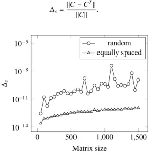
In a first numerical experiment we want to test the sensitivity and robustness of the reduction procedure to sym-metric form. The test matrices were generated as in Section 4, but this time we consider both matrices with random (uniformly distributed between 0 and 1) and equally spaced (minimal gap equal to 0.05) eigenvalues. The two plots in Figure 3 show the symmetry ofCdepending on the size of the problem, measured as
∆s= kC−CTk kCk . 0 500 1,000 1,500 10−14 10−11 10−8 10−5 Matrix size ∆s random equally spaced
Figure 3: Symmetry of the matrixCfor random and equally spaced eigenvalues.
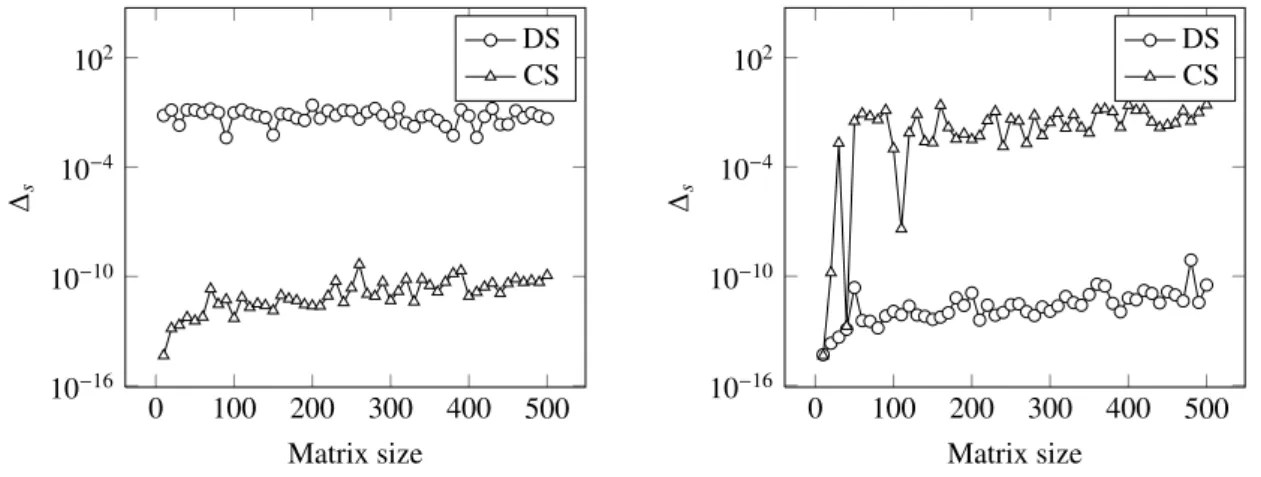
Keeping in mind that “large” off-diagonal entries do not guarantee the eigenvalues to be distinct, we want to know how bad the consequences can be for the symmetrization methods. We considered both our and Ikramov’s method (DS) [13] to compute the unitary similarity to complex symmetric form. Both methods rely on the hypothetical zeros appearing on the off-diagonals to determine whether the matrix has multiple eigenvalues or not. Problems might arise when the eigenvalues of the considered matrices have some peculiar feature: for instance, the method presented in this paper could have difficulties in dealing with a normal matrix having distinct eigenvalues with equal absolute values; on the other hand, DS could fail if some eigenvalues have equal real or imaginary parts.
We present the results of two experiments concerning the two special settings mentioned above. The symmetry of the resulting matrixCwas estimated as before. First we consider matrices having two pairs of eigenvalues with equal real and imaginary part respectively. These are not problematic for our method as long as their absolute values remain distinct. On the contrary, DS relies on the Toeplitz decompositionN =H1+ıH2of the matrix; the current setting is
thus troublesome, because bothH1andH2have multiple eigenvalues. Indeed, the first plot in Figure 4 clearly shows
Next we consider matrices with one pair of distinct eigenvalues having the same absolute value. As we would expect DS performs well while our method occasionally works, as can be seen in the second plot. Note that this time the error is only related to the submatrixC(1 :n−1,1 :n−1) wherenis the problem size, as we can only ensure a block structure. 0 100 200 300 400 500 10−16 10−10 10−4 102 Matrix size ∆s DS CS 0 100 200 300 400 500 10−16 10−10 10−4 102 Matrix size ∆s DS CS
Figure 4: Comparing symmetry obtained in two special settings by our method and DS.
6.2. Accuracy
As we illustrated in the previous section, numerical issues can compromise the correct behavior of the method. Nonetheless the novel approach is quite satisfactory, with very good results in terms of accuracy for several problems. For instance, for normal matrices having one double singular value and minimum distance between distinct singular values equal to 1. We generated such kind of matrices as in Section 4, and computed eigenvalue decompositions of the diagonal blocks via the Takagi factorization as in Section 3.2 via twisted factorization or QR-based methods. The Jacobi method is then reduced to a single rotation, that annihilates the two nonzero off-diagonal entries.
0 500 1,000 1,500 10−13 10−12 Matrix size (n) ∆s 0 500 1,000 1,500 10−15 10−13 10−11 10−9 Matrix size Error ∆QR λ ∆T F λ ∆eig
Figure 5: Symmetry of the matrixCand relative eigenvalue errors.
The new approach was proved to be reliable both in terms of symmetry ofCand of accuracy of the computed eigenvalues, even outperforming Matlab’seigcommand results. Figure 5 shows an estimate of∆s, defined as in
7. Conclusions and future work
In this article a novel approach to compute the eigenvalues of normal matrices was presented. The simplest case, where the intermediate matrix is symmetric, showed overall, good numerical performance, both with respect to speed as well as accuracy. The theoretical framework to process the more complex case seems promising, but can suffer significantly from numerical pitfalls.
The article opens several new directions for extending the current research. In Section 4 we relied entirely on existing algorithms to compute the SSVD factorization. These algorithms are constructed, however, for generic symmetric matrices and do not exploit the fact that the input matrix is also normal. We remark that normality is lost transforming the symmetric matrix to symmetric tridiagonal form.
Furthermore, a matrix is normal and symmetric if and only if it admits a real orthogonal eigenvalue decomposition, see [12, Problem 57,§2.5]. Unfortunately, the algorithm presented in this paper is not able to produce a real orthogonal matrix, except when the original matrix itself is real. Determining if it is possible to achieve the same result while using only real orthogonal transformations is still an open question.
The block case needs more attention: it is still unclear for which distribution of eigenvalues and singular values the method will work fine.
8. Acknowledgements
We wish to thank Prof. Roger Horn for bringing to our attention some general conditions for complex symmetry, formulated in this paper as Lemma 4 and Theorem 9. His valuable comments and helpful suggestions greatly improved the presentation of the results in Section 3.1.
We would also thank the anonymous referee for his/her many precious comments and for calling our attention to [13].
9. Bibliography
[1] G. S. Ammar, W. B. Gragg, and L. Reichel. On the eigenproblem for orthogonal matrices. InProceedings of the 25th IEEE Conference on Decision&Control, pages 1963–1966. IEEE, New York, USA, 1986.
[2] L. Balayan and S. R. Garcia. Unitary equivalence to a complex symmetric matrix.Operators and Matrices, 4:53–76, 2010.
[3] A. Bunse-Gerstner and L. Elsner. Schur parameter pencils for the solution of the unitary eigenproblem.Linear Algebra and its Applications, 154-156:741–778, 1991.
[4] A. Bunse-Gerstner and W. B. Gragg. Singular value decompositions of complex symmetric matrices.Journal of Computational and Applied Mathematics, 21:41–54, 1988.
[5] I. S. Dhillon and B. N. Parlett. Multiple representations to compute orthogonal eigenvectors of symmetric tridiagonal matrices. Linear Algebra and its Applications, 387:1–28, 2004.
[6] L. Elsner and Kh. D. Ikramov. Normal matrices: An update.Linear Algebra and its Applications, 285:291–303, 1998. [7] M. Fiedler. A characterization of tridiagonal matrices.Linear Algebra and its Applications, 2:191–197, 1969.
[8] S. R. Garcia, D. E. Poore and M. K. Wyse. Unitary equivalence to a complex symmetric matrix: a modulus criterion.Operators and Matrices, 5:273–287, 2011.
[9] H. H. Goldstine and L. P. Horwitz. A procedure for the diagonalization of normal matrices.Journal of the ACM, 6(2):195, 1959. [10] G.H. Golub and C. F. Van Loan.Matrix Computations. Johns Hopkins University Press, Baltimore, Maryland, USA, third edition, 1996. [11] R. Grone, C. R. Johnson, E. M. Sa, and H. Wolkowicz. Normal matrices.Linear Algebra and its Applications, 87:213–225, 1987. [12] R. A. Horn and C. R. Johnson.Matrix Analysis, 2nd ed.. Cambridge University Press, Cambridge, 2013.
[13] Kh. Ikramov. Symmetrization of complex normal matrices.Computational Mathematics and Mathematical Physics, 33:837–842, 1993. [14] C. G. J. Jacobi. ¨Uber ein leichtes Verfahren, die in der Theorie der S¨acularst¨orungen vorkommenden Gleichungen numerisch afzul¨osen.
Journal f¨ur die reine und angewandte Mathematik, 30:51–94, 1846.
[15] G. Loizou. On the quadratic convergence of the Jacobi method for normal matrices.The Computer Journal, 15(3):274, 1972.
[16] F. T. Luk, S. Qiao. A fast singular value algorithm for Hankel matrices.Fast Algorithms for Structured Matrices: Theory and Applications, Contemporary Mathematics, 323:169–177, 2001
[17] A. Ruhe. Closest normal matrix finally found!BIT, 27:585–598, 1987.
[18] T. Takagi. On an algebraic problem related to an analytic theorem of Carath´eodory and Fej´er and on an allied theorem of Landau.Japanese Journal of Mathematics, 1:82–93, 1924.
[19] H. A. van der Vorst.Computational methods for large eigenvalue problems. Elsevier, North Holland, 2001.
[20] R. Vandebril. A unitary similarity transform of a normal matrix to complex symmetric form. Applied Mathematics Letters, 24:160–164, 2011.
[21] J. Vermeer. Orthogonal similarity of a real matrix and its transpose.Linear Algebra and its Applications, 428:382–392, 2008. [22] D. S. Watkins.The Matrix Eigenvalue Problem: GR and Krylov Subspace Methods. SIAM, Philadelphia, USA, 2007.
[23] J. H. Wilkinson.The Algebraic Eigenvalue Problem. Oxford University Press, New York, USA, 1978.
[24] W. Xu and S. Qiao. A divide-and-conquer method for the Takagi factorization.SIAM Journal on Matrix Analysis and Applications, 30(1):142– 153, 2008.
[25] W. Xu and S. Qiao. A twisted factorization method for symmetric SVD of a complex symmetric tridiagonal matrix. Numerical Linear Algebra with Applications, 16(10):801–815, 2009.