Data-Driven Control with Learned Dynamics

(1)

Clemson University Clemson University

TigerPrints

All Theses Theses

August 2020

Data-Driven Control with Learned Dynamics

Wenjian Hao

Clemson University, [email protected]

Follow this and additional works at: https://tigerprints.clemson.edu/all_theses

Recommended Citation Recommended Citation

Hao, Wenjian, "Data-Driven Control with Learned Dynamics" (2020). All Theses. 3398.

https://tigerprints.clemson.edu/all_theses/3398

This Thesis is brought to you for free and open access by the Theses at TigerPrints. It has been accepted for inclusion in All Theses by an authorized administrator of TigerPrints. For more information, please contact

(2)

Data Driven Control with Learned Dynamics

A Thesis Presented to the Graduate School of

Clemson University In Partial Fulfillment

of the Requirements for the Degree Master of Science Mechanical Engineering by Wenjian Hao August 2020 Accepted by:

Dr. Yue Wang, Committee Chair Dr. Yiqiang Han, Research Chair

(3)

Acknowledgments

The past two years at Clemson University have been a great journey in my life. During this period, I obtained not only lots of technical knowledge but also a massive help and happy memories from the university community, here I would like to express my sincere gratitude to those who helped me.

First of all, I would like to thank my advisor, Dr. Yiqiang Han, for introducing me to the fields of deep reinforcement learning, dynamical systems, and control. I am very grateful for the opportunity to get involved with many incredible CI projects like autonomous drones and autonomous race cars. I learned a lot of cutting edge knowledge and got much successful experience while doing these great projects. I also appreciate my committee members, Dr. Yue Wang and Dr. Mohammad Naghnaeian, for their guidance and support. Likewise, I would like to thank Professor Umesh Vaidya for his critical input and advice when we worked together to develop a novel algorithm that combines deep neural network and Koopman operator.

My gratitude also goes to my colleagues and friends who offered me help and cooperated for class team projects. It is you who makes my experience unforgettable and precious.

Finally, I would like to express my gratitude to the people dearest to me. I want to thank my parents and family for their love, support, and wisdom throughout my life. Thank you for being part of this journey, even when being at a distance.

(4)

Abstract

This research focuses on studying data-driven control with dynamics that are actively learned from machine learning algorithms. With system dynamics being identified using neural networks either explicitly or implicitly, we can apply control following either a model-based approach or a model-free approach. In this thesis, the two different methods are explained in detail and finally compared to shed light on the emerging data-driven control research field.

In the first part of the thesis, we first introduce state-of-art Reinforcement Learning (RL) algorithm representing data-driven control using a model-free learning approach. We discuss the advantages and shortcomings of the current RL algorithms and motivate our study to search for a model-based control which is physics-based and also provides better model interpretability. We then propose a novel data-driven, model-based approach for the optimal control of the dynamical system. The proposed approach relies on the Deep Neural Network (DNN) based learning of Koopman operator and therefore is named as Deep Learning of Koopman Representation for Control (DKRC). In particular, DNN is employed for the data-driven identification of basis function used in the linear lifting of nonlinear control system dynamics. One a linear representation of system dynamics is learned, we can implement classic control algorithms such as iterative Linear Quadratic Regulator (iLQR) and Model Predictive

(5)

driven and does not rely on prior domain knowledge. The OpenAI Gym environment is used for simulations of various control problems. The method is applied to three classic dynamical systems on OpenAI Gym environment to demonstrate the capability.

In the second part, we compare the proposed method with a state-of-art model-free control method based on an actor-critic architecture – Deep Deterministic Policy Gradient (DDPG), which has been proved to be effective in various dynamical systems. Two examples are provided for comparison, i.e., classic Inverted Pendulum and Lunar Lander Continuous Control. We compare these two methods in terms of control strategies and the effectiveness under various initialization conditions from the results of the experiments. We also examine the learned dynamic model from DKRC with the analytical model derived from the Euler-Lagrange Linearization method, demonstrating the accuracy in the learned model for unknown dynamics from a data-driven sample-efficient approach.

Key Words: Dynamical System and Control, Koopman Operator,

Rein-forcement Learning, Deep Deterministic Policy Gradient (DDPG), Model Predictive Control (MPC), Deep Neural Network (DNN)

(6)

List of Tables

(9)

List of Figures

1.1 Simple neural network structure example. n: The dimension of the

input observations N: The dimension of lifted observations . . . 3

1.2 Deep Koopman Representation for Control (DKRC) framework with comparison to Reinforcement Learning . . . 3

1.3 Koopman Operator Scheme . . . 5

1.4 Schematics of DDPG framework . . . 8

2.1 The first failure solution flow chart . . . 16

2.2 The Second failure solution flow chart . . . 17

3.1 Koopman Operator Learning using Neural Network Scheme . . . 21

3.2 Eigenfunctions learned from uncontrolled case, Left: real part of eigen-functions, Right: imaginary part of the eigenfunctions. The dominant eigenfunction has zero value imaginary part. . . 25

3.3 Eigenfunctions learned from controlled case, Left: real part of eigen-functions, Right: imaginary part of the eigenfunctions. The dominant eigenfunction has zero value imaginary part. . . 25

3.4 Schematics of DKRC framework . . . 27

4.1 Inverted Pendulum . . . 30

4.2 Trajectories of Swinging Pendulum under Control using trained DDPG reinforcement learning model. The figure exhibits the trajectories of the tip of the pendulum breaking through Hamiltonian energy level lines to arrive at the goal position (θ = 0,θ˙= 0) . . . 31

4.3 Trajectories of Swinging Pendulum under control using DKRC model (left) vs. DDPG RL model (right) initialized at the same state . . . . 32

4.4 Example 3D deployment trajectory from DKRC (left) and Reinforce-ment Learning (right), colormapped by the magnitude of energy . . . 33

4.5 100 games recorded reward using DKRC . . . 34

4.6 Acrobot . . . 35

4.7 DKRC deployment trajectories of Acrobot under Control. As shown in the picture, the green line is goal line for second link.The goal of this game is to touch the green line with the second link . . . 37

4.8 100 games recorded reward using DKRC . . . 38

(10)

4.10 Balance keeping process for one game using DKRC . . . 39 4.11 100 games recorded reward using DKRC . . . 40 4.12 Lunar Lander . . . 41 4.13 DKRC deployment for ten games, Red point: starting point, Blue point:

goal position . . . 42 4.14 Data visualization of the training sample for Lunar Lander environment.

The 1876 data pairs are obtained from playing five games. The different color gradient represents different state observations and control inputs collected. Each row on Left figure denotes one of six states; right figure shows the control input from main and side engine thrusts . . . 43 5.1 Environment visualization . . . 46 5.2 Trajectories of Swinging Pendulum implementing DDPG model (left)

vs. DKRC model (right) initialized at the lowest position . . . 50 5.3 Trajectories of Swinging Pendulum implementing DDPG model (left)

vs. DKRC model (right) initialized at the left horizontal position . . . 51 5.4 Trajectories of Swinging Pendulum implementing DDPG model (left)

vs. DKRC model (right) initialized at the right horizontal position . . . 51 5.5 Trajectories of Swinging Pendulum implementing DDPG model (left)

vs. DKRC model (right) initialized at the close left upright position . 52 5.6 Trajectories of Swinging Pendulum implementing DDPG model (left)

vs. DKRC model (right) initialized at the close right upright position 52 5.7 50 pendulum games data recorded using DDPG model (left) vs. DKRC

model (right), color mapped by energy . . . 53 5.8 DDPG(left) vs. DKRC(right): Recorded Observations & Energy . . . 54 5.9 Schematics of autoencoder neural network sturcture of DKRC . . . . 56 5.10 DKRC’s planned trajectory and actually executed trajectory in Inverted

pendulum . . . 57 5.11 Lunar Lander Environment . . . 58 5.12 DKRC’s planned trajectory and actual executed trajectory in Lunar

Lander, color mapped by the distance between the planned point and the executed point . . . 59 5.13 Five pendulum games with input states noise using DDPG (left) vs.

DKRC (right) solutions . . . 60 5.14 One pendulum game using DKRC model (left) vs. Euler-Lagrange

method (right); Both tests initialized at θ0 = ₁₈π, θ˙0 = 0.5 . . . 62

1 Neural Network Structure For Inverted Pendulum . . . 67 2 Neural Network Structure For Double Pendulum Balancing on a Cart 68 3 Neural Network Structure For Lunar Lander Control . . . 68 4 Neural Network Structure For Acrobot Swing Up . . . 69

(11)

Chapter 1 Introduction

The data-driven control of dynamical systems has been an emerging research area with various applications in robotics, manufacturing systems, autonomous vehi-cles, and transportation networks. There is a rising interest in shifting from completely model-based to data-driven control paradigm with the increasing complexity of en-gineered systems and easy access to a large amount of sensor data. One successful example is the Deep Reinforcement Learning (DRL), which consists of deploying Deep Neural Networks (DNN) to learn optimal control policy. It is arising as one of the powerful tools for data-driven control of dynamic systems [37]. However, the downside of only relying on a neural network approach is also obvious. The use of DNN is often being called a "black-box" approach. The problem of control design for a system with nonlinear dynamics is recognized to be a particularly challenging problem. More recently, the use of linear operators from the ergodic theory of dynamical systems has offered some promises towards providing a systematic approach for nonlinear control [4, 16, 20, 24, 26, 28, 30, 33, 34, 39, 40].

The controller synthesis for dynamic systems in the model-based and model-free setting has a long history in control theory literature. However, some challenges need

(12)

to be overcome for the successful extension of linear operator-based analysis methods to address the synthesis problem. The basic idea behind the linear operator framework involving Koopman and Perron-Frobenius operator is to lift the finite-dimensional nonlinear dynamics to infinite-dimensional linear dynamics. The finite-dimensional approximation of the linear operator is obtained using the time series data of the dynamic system.

One of the main challenges is the selection of appropriate choice of finite basis functions used in the finite but high dimensional linear lifting of nonlinear dynamics. The standard procedure is to make a prior choice of basis function such as radial basis function or polynomial function for the finite approximation of the Koopman operator. However, such an approach often does not take advantage of the known physics or the data in choosing the basis function.

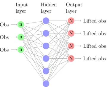
An alternate approach based on the power of Deep Neural Network (DNN) could be used for the data-driven identification of the appropriate basis function in the autonomous (uncontrolled) setting [21, 47]. A dummy representation of the Deep Neural Network (DNN) structure is shown in Figure 1.1.

The conjecture is that physics is reflected in the data, and DNNs are efficient in exploiting the power of the data. In this work, we extend the application of DNN for the selection of basis functions in a controlled dynamical system setting.

The main contributions of our method are as follows. We extend the use of DNN for the finite-dimensional representation of the Koopman operator in a controlled dynamical system setting. Our data-driven learning algorithm can automatically search for a rich set of suitable basis functions to construct the approximated linear model in the lifted space. The OpenAI Gym environment is employed for data generation and training of DNN to learn the basis functions [3]. Example systems

(13)

n Obs n Obs n Obs N Lifted obs N Lifted obs N Lifted obs N Lifted obs Hidden layer Input layer Output layer

Figure 1.1: Simple neural network structure example. n: The dimension of the input observations N: The dimension of lifted observations

control is used to demonstrate the capability of the developed framework. This work is on the frontier to bridge the understanding of model-based control and model-free control (e.g. Reinforcement Learning) from other domains. The proposed comparison framework between the two approaches is depicted in Figure 1.2.

Nonlinear System w/ Continuous Control

Linear Predictor from DNN Model Predictive Control

This Study ℝ𝑛_{⇒ ℝ}𝑁 𝑧𝑡+1= 𝐴𝑧𝑡+ 𝐵𝑢𝑡 𝑧0= 𝜓 𝑥0 ℒ ≔ ෍ 𝑡=1 𝑇 𝒀𝒍𝒊𝒇𝒕− 𝐴𝑿𝒍𝒊𝒇𝒕− 𝐵𝑼 _𝐹+ 𝜆1𝑨1+ 𝜆2 𝑩1 PAST Future Actor-Critic Framework Reinforcement Learning ℝ𝑛 max_𝜃 𝔼𝜏~𝑝𝜃𝜏 ෍ 𝑡 𝑟 𝑠𝑡, 𝑎𝑡 Model-Free Control Design Action for Max. Cumulative Rewards

Figure 1.2: Deep Koopman Representation for Control (DKRC) framework with comparison to Reinforcement Learning

(14)

1.1 Koopman Operator

The following sections introduce several key concepts of algorithms and the state-of-art research progress in those areas.

Koopman operator theory is an alternative formalism for dynamical systems theory, which offers excellent utility in the analysis and control of nonlinear and high-dimensional systems using data [25]. Koopman operator is an infinite-high-dimensional linear operator that can transfer a nonlinear system to a high-dimensional linear system. It fully captures all properties of the underlying dynamical system provided that the space of observables f(xt) contains the components of the states xt [20].

Considering an uncontrolled dynamic system in Equation 1.1.

xt=f(xt) (1.1)

The Koopman operator K would be used to transform the representation of the system in the following format as shown in Equation 1.2. The detailed use of this linear representation will be introduced in later sections together with the proposed model-based control design.

(Kψ) =ψ(F(x)) (1.2)

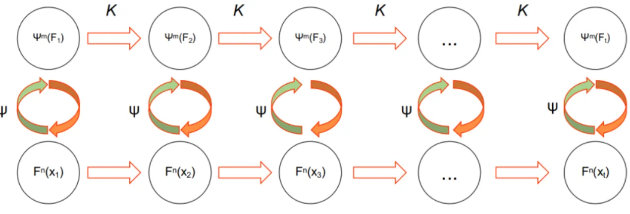
A simple explanation diagram of Koopman Operator is exhibited in Figure 1.3. As shown in the figure, the K is the koopman operator, ψ represents an infinite dimensional basis function,F(xt)is the state evolution operator,ψ(F(xt))is the linear

lifted observation space, n is the dimension of the observation, m is the dimension of the lifted observation, Therefore, Koopman operator is defined as the composition of

(15)

Figure 1.3: Koopman Operator Scheme

1.2 Model Predictive Control

Model predictive control (MPC) is an advanced method of process control that is used to control a process while satisfying a set of constraints. Model predictive controllers rely on dynamic models of the process, most often linear empirical models obtained by system identification. The main advantage of MPC is the fact that it allows the current timeslot to be optimized, while keeping future timeslots in account. This is achieved by optimizing a finite time-horizon, but only implementing the current timeslot and then optimizing again, repeatedly, thus differing from Linear-Quadratic Regulator (LQR). Also MPC has the ability to anticipate future events and can take control actions accordingly. PID controllers do not have this predictive ability. MPC is nearly universally implemented as a digital control, although there is research into achieving faster response times with specially designed analog circuitry [42].

In this study, we implement the Model Predictive Control (MPC) after learning the dynamics of the lifted high-dimensional linear system with DKRC. Other methods, such as regression or DAGGER (i-LQR or MCTS for planning) techniques have been introduced after the learned model is available. However, those methods suffer from

(16)

distribution mismatch problems or issues with the performance of open-loop control in stochastic domains. We propose using MPC iteratively, which can provide robustness to small model errors that benefit from the close loop control. As mentioned by authors in Ref [6], if the system dynamics were to be linear and the cost function convex, the global optimization problem solved by MPC methods would be convex (To solve the convex problem, we used CVXPY [8] in this study.). Under this assumption, the convex programming optimization techniques could be promising to achieve some theoretical guarantees of convergence to an optimal solution. Therefore MPC would undoubtedly perform better in a linear setting. MPC is an online optimization solver method that seeks optimal state solutions at each time step under certain defined constraints. Therefore it features closed-loop planning, which exhibits higher robustness than other simpler models. It has been proven to be tolerant of the modeling errors within Adaptive Cruise Control(ACC) simulation [10] [49]. MPC represents the state-of-the-art for the practice of real-time optimal control [22].

1.3 Reinforcement Learning

To compare the advantages and disadvantages of the proposed model-based method, we examine the proposed method with another model-free control method (Deep Deterministic Policy Gradient) in the second part of this study. Deep

Deter-ministic Policy Gradient (DDPG) is a reinforcement learning algorithm based on an actor-critic framework. The DDPG and its variants have been demonstrated to be very successful in designing optimal continuous control for many dynamical systems. However, compared to the above model-based optimal control, DDPG employs a more black-box style neural network structure that outputs control directly based on learned

(17)

of training data and a good design of the reward function to achieve good performance without learning an explicit model of the system dynamics. We use this section to introduce several of the key concepts to better understand this state-of-the-art reinforcement learning algorithm.

1.3.1 Deep Deterministic Policy Gradient

Deep Deterministic Policy Gradient (DDPG) is a model-free, off-policy algo-rithm, which uses DNN function approximators to learn policies in high-dimensional, continuous action spaces [38]. DDPG is a combination of the deterministic policy gradient approach and insights from the success of Deep Q Network (DQN) [27]. DQN is a policy optimization method that achieves optimal policy by inputting observation and updates policy by back-propagate policy gradients. However, DQN can only handle discrete and low-dimensional action spaces, limiting its application considering many control problems have high-dimensional observation space and continuous control requirements. The innovation of DDPG is that it extends the DQN to continuous control domain and higher dimensional system and has been claimed that it robustly solves more than 20 simulated physics tasks, including classic problems such as cart-pole swing-up, dexterous manipulation, legged locomotion and car driving [38]. In addition, DDPG has been demonstrated to be sample-efficient compared to the Covariance Matrix Adaptation Evolution Strategy (CMA-ES), which is also a black-box optimization method widely used for robot learning [1].

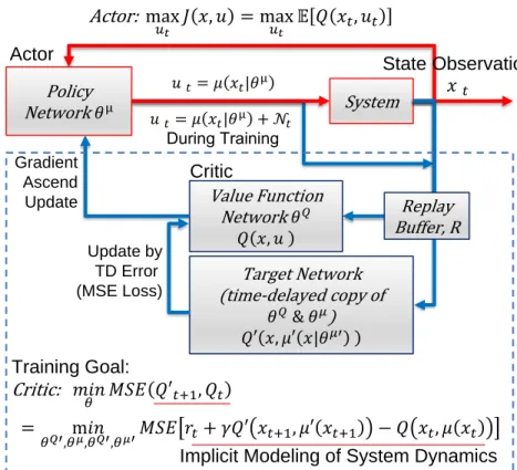
A schematic diagram of the DDPG framework is shown in Figure 1.4.

The control goal of the DDPG algorithm is to find control actionuto maximize the rewards (Q-values) evaluated at the current time step. The training goal of the algorithm is to learn neural network parameters for the above networks so that rewards

(18)

System 𝑢𝑡= 𝜇 𝑥𝑡|𝜃μ 𝑥_𝑡 Policy Network 𝜃μ State Observation Value Function Network 𝜃𝑄 𝑄 𝑥, 𝑢 Target Network (time-delayed copy of 𝜃𝑄& 𝜃𝜇) 𝑄′ 𝑥, 𝜇′ 𝑥|𝜃𝜇′ 𝑢_𝑡= 𝜇 𝑥_𝑡|𝜃μ _{+ 𝒩} 𝑡 During Training Actor Critic Update by TD Error (MSE Loss) Gradient Ascend Update Control Goal: Actor: max 𝑢𝑡 𝐽 𝑥, 𝑢 = max 𝑢𝑡 𝔼 𝑄 𝑥𝑡, 𝑢𝑡 Training Goal: Critic: 𝑚𝑖𝑛 𝜃 𝑀𝑆𝐸 𝑄′𝑡+1, 𝑄𝑡 = m𝑖𝑛 𝜃𝑄′_,𝜃𝜇_,𝜃𝑄′_,𝜃𝜇′𝑀𝑆𝐸 𝑟𝑡+ 𝛾𝑄′ 𝑥𝑡+1, 𝜇′ 𝑥𝑡+1 − 𝑄 𝑥𝑡, 𝜇 𝑥𝑡 Implicit Modeling of System Dynamics

Replay Buffer, R

Figure 1.4: Schematics of DDPG framework

can be maximized at each sampled batch, while still being deterministic. The training of the DDPG network will then follow a gradient ascend update from each iteration, as defined in Equation 1.3

∇θµJ ≈_E[∇_θµQ(x, u|θQ)|x=x_t, u=µ(x_t|θµ)] (1.3)

In Equation 1.3, we have two separate networks involved: Value function network θQ _{and policy network} _θµ_{. To approximate the gradient from those two}

(19)

networks: Actor, Critic, Target Actor, Target Critic.

At the gathering training samples stage, we use a replay buffer to store samples. A replay buffer of DDPG essentially is a buffered list storing a stack of training samples (xt, ut, rt, xt+1). During training, samples can be drawn from the replay buffer

in batches, which enables training using a batch normalization method [5]. For each stored sample vector,t is current time step, xis the collection of state observations at current time step t,r is numerical value of reward at current state,u is the action of time step t, and finally, the xt+1 is the state in the next time step t+ 1 as a result of

taking action ut at state xt. Replay buffer makes sure an independent and efficient

sampling [7].

As discussed above, the DDPG framework is a model-free reinforcement learning architecture, which means it does not seek an explicit model for the dynamical system. Instead, we use a value function network, also called Critic network Q(s, a|θQ), to approximate the result from a state-action pair. The result of a trained Critic network estimates the expected future reward by taking action ut at state xt. If we take the

gradient of the change in the updated reward, we will be able to use that gradient to update our Policy network, also called Actor network. At the end of the training, we obtain an Actor network capable of designing optimal control based on past experience. Since there are two components in the formulation of the gradient of reward in Equation 1.3, we can apply the chain rule to break the process into evaluating gradients from Actor and Critic networks separately. The total gradient is then defined as the mean of the gradient over the sampled mini-batch, where N is the size of the training mini-batch taken from replay buffer R, as shown in Equation 1.4. Silver et al. showed proof in Ref. [31] that Equation 1.4 is the policy gradient that can guide the DDPG

(20)

model to search a policy network to yield the maximum expected reward. ∇θµJ ≈ 1 N X t [∇uQ(x, u|θQ)|x=xt,u=µ(xt)∇θµµ(x|θ µ )|xt] (1.4)

In this case, dynamical responses from the system are built into the modeling of the Critic network, thus indirectly modeled. The accuracy in predicted reward values is used as the only training criterion in this process, signifying the major difference between the model-free reinforcement learning and the model-based optimal control method such as DKRC. Some of the later observations in different behaviors from model-based vs. model-free comparison have roots stemming from this fundamental difference.

We separate the training of the DDPG into the training of the Actor and Critic networks.

Actor, or policy network (θµ_{), is a simple neural network with weights}_θµ_{, which}

takes states as input and outputs control based on a trained policy µ(x, u|θµ₎_{. The}

Actor is updated using the sampled policy gradient generated from the Critic network, as proposed in Ref. [32].

Critic, or value function network, is a neural network with weights θQ, which takes a state-action pair (xt, ut)as input. We define a temporal difference error term,

et (TD error), to track the error between the current output compared to a target

Critic network with future reward value using future state-action pair as input in the next time step. The total loss from the Critic network during a mini-batch is defined as L in Equation 1.5, which is based on Q-learning, a widely used off-policy

(21)

algorithm [41]. et= (rt+γQ 0 (xt+1, µ 0 (xt+1|θµ 0 )|θQ 0 ))−Q(xt, ut|θQ) L= 1 N X t et2 (1.5) In this Critic loss function in Equation 1.5, the terms with prime symbol (0) is the Actor/Critic model from the target networks. Target Actor µ0 and target Critic Q0 of DDPG are used to sustain a stable computation during the training process. These two target networks are time-delayed copies of the actual Actor/Critic networks in training, which only take a small portion of the new information from the current iteration to update target networks. The update scheme of these two target networks are defined in Equation 1.6, where τ is Target Network Hyper Parameters Update rate super parameter with a small value (τ 1) to improve the stability of learning.

θQ 0 ←τ θQ+ (1−τ)θQ 0 θµ 0 ←τ θµ+ (1−τ)θµ 0 (1.6)

To train DDPG, we initialize four networks (Q(s, a|θQ₎_{, µ}₍_s_|_θµ₎_{, Q}0₍_{s, a}_|_θQ0₎_{, µ}0₍_s_|_θµ0₎₎

and a list buffer (R) first, then select an initial action from actor, executing action

at and observe reward rt and new state st+1, store (st, at, rt, st+1) in the buffer R,

sampling mini training batch input randomly from R, updating critic by Equation 1.5, updating actor by Equation 1.4, updating target actor and critic by Equation 1.6 until loss value converges.

(22)

1.4 Thesis Organization

The work will be presented in the following order: Ch 2 introduces the proposed problem setup; Ch 3 formulates the proposed algorithm; Ch 4 details the results and discussions from the deployment of proposed algorithm; In Ch 5, since DKRC and DDPG are both capable of solving dynamic systems control problems with high-dimensional and continuous control space, direct comparison is desirable by constructing the two algorithms from the ground up and applying them to solve the same tasks. In this chapter, we also compare the DKRC to the analytical model obtained by the classic Euler-Lagrange Linearization method. The comparison are examined in the Inverted pendulum environment and Lunar Lander Continuous Control environment in OpenAI Gym [3]. Ch 6 concludes the thesis.

(23)

Chapter 2 Research Problem Setup

This chapter consists of the processes we have taken to develop the algorithm. We generally attempt three different ways to solve the proposed research problem, two of them failed, and only one succeeded in the end.

2.1 Problem Set-up

Consider a discrete-time, nonlinear dynamical system along with a set of observation data of length T:

xt+1 =F(xt, ut)

X = [x1, x2, . . . , xT], Y = [y1, y2, ..., yT], U = [u1, u2, . . . , uT]

(2.1) where, xt ∈Rn, ut∈Rm is the state and control input respectively, and yt =xt+1 for t= 1, . . . , K. The objective is to provide a linear lifting of the nonlinear dynamical system for the purpose of control. The Koopman operator theory can be used to lift the nonlinear control dynamics to linear control dynamics. The Koopman operator (K) is an infinite-dimensional linear operator defined on the space of functions as

(24)

follows:

[Kg](x) =g◦F(x, u) (2.2) For more details on the theory of Koopman operator in a dynamical system and control setting, refer to Ref. [19, 43, 45, 46]. Related work on extending Koopman operator methods to controlled dynamical systems can be found in References [2, 16, 17, 20, 23, 29, 48]. While the Koopman based lifting for the autonomous system is well understood and unique, the dynamical system can be lifted in different ways. In particular, for the control of affine system, the lifting in the functional space will be bi-linear [15, 23]. Given the computational focus of this paper, we resort to the linear lifting of the control system. The linear lifting also has the advantage of using state of the art control methodologies such as linear quadratic regulator (LQR) and Model Predictive Control (MPC) from linear system theory. The linear lifting of nonlinear control system is given by

Ψ(xt+1) = AΨ(xt) +But (2.3)

where Ψ(x) = [ψ1(x), . . . , ψN(x)]> ∈ RN >>n is the state or the basis in the

lifted space. The matrix A ∈ _RN×N _and _B _∈

RN×m are the finite dimensional

approximation of the Koopman operator for control system in the lifted space. One of the main challenges in the linear lifting of the nonlinear dynamics is the proper choice of basis functions used for lifting. While the use of radial basis function, polynomials, and kernel functions is most common, the choice of appropriate basis function is still open. Lack of systematic approach for the selection of appropriate basis has motivated

(25)

the use of Deep Neural Network (DNN) for data-driven learning of basis function. The use of DNN has been explored for the learning of basis functions in uncontrolled settings.

The planned control inputs considered in this study are in continuous space and later will be compared to state-of-art model-free learning methods such as Reinforce-ment Learning. An overview of the scope of this work is shown in Figure 1.2. Both the two methods (our Deep Koopman Representation for Control (DKRC) approach and Reinforcement Learning) apply a data-driven model-free learning approach to learn the dynamical system. However, our approach seeks a linear representation of nonlinear dynamics and then design the control using a model-based approach, which will be discussed in later sections.

2.2 Proposed Solutions

In this section, we demonstrate how we develop the algorithm, and the processes are divided into three attempts.

2.2.1 The First Solution

In order to solve the problem defined in Equation 2.3. Firstly, We attempt to use three neural networks (ψ(xt+1|θ), A(ψ(xt|θ)|θA), B(ut|θB)) to get a solution for

Equation 2.3, which transfers the loss function of the training process to Equation 2.4.

(26)

Where, A(ψ(xt|θ)|θA) takes the output of ψ(xt+1|θ) as input state and outputs the

same dimensional lifted state asψ(xt+1|θ). A scheme of the attempt is shown in Figure

2.1.

Figure 2.1: The first failure solution flow chart

The problem of this attempt is that: (1) To get A, B matrices, we can not add any layer and bias in neural networks A(ψ(xt|θ)|θA) andB(ut|θB), which leads to an

imprecise result. (2) Besides, we find that when the neural networks are trained to minimize the loss function using gradients back-propagation, it tends to simply push all three neural networks’ outputs close to zero, which is one of the reasons why the solution only takes trivial control no matter what states it accepted during result test.

2.2.2 The Second Solution

In this solution, we only use one neural networkψ(xt+1|θ)to solve Equation

2.3. At training epoch n, loss function is defined in Equation 2.5.

(27)

Where, An, Bn is defined in Equation 2.6 and A1, B1 is randomly generated at the

first training epoch.

[An, Bn] = 1 L L X t=1 ψt+1    ψt ut       ψt ut    ψt ut       † (2.6) where, L is the number of training samples,† denotes psedoinverse.

When n > 1, A, B is updated as following:

An =An+ (1−)An−1, Bn =Bn+ (1−)Bn−1, 1

is selected to get a smooth parameter update. A general solution flow chart is exhibited in Figure 2.2.

Figure 2.2: The Second failure solution flow chart

The problem of this solution is that: (1) The loss function will converge after the first epoch as a result of that the A, B matrices are obtained mathematically; (2) Besides, the tiny loss value is also a challenging work for neural networks to update its parameters, which means it is hard to converge after the first training epoch. The result of this solution is that it cannot take reasonable control and fails at each game.

(28)

2.3 Lessons Learned

After the above two failed attempts, we decided to use only one neural network to represent all the training terms and only update the A, B matrices after the entire training process converges. We also integrate another loss function to ensure the lifted highdimensional linear system controllable, which is concluded in the next chapter -Algorithm Proposed.

(29)

Chapter 3 Algorithm Proposed

This chapter exhibits details of the data-driven control algorithm we develop and also shows the eigenfunctions gotten by the algorithm in the swing-up pendulum system with/without control.

3.1 Deep Learning of Koopman Representation for

Control

To enable deep Koopman representation for control, the first step is to use the DNN approach to approximate Koopman operator for control purposes. Our method seeks a multi-layer deep neural network to automate the process of finding the basis function for the linear lifting of nonlinear control dynamics via Koopman operator theory. Each feed-forward path within this neural network can be regarded as a nonlinear basis function (ψi :Rn→R), whereas the DNN as a collection of basis

functions can be written as Ψ : _Rn _→

RN. Each output neuron is considered as a

compounded result from all input neurons. Therefore, the mapping ensures that our Koopman operator maps functions of state space to functions of state space, not states

(30)

to states.

Unlike existing methods used for the approximation of the Koopman operator, where the basis functions are assumed to be known apriori, the optimization problem used in the approximation of Koopman operator using DNN is non-convex. The non-convexity arises due to simultaneous identification of the basis functions and the linear system matrices. The setup of our DNN training process is listed below to address this concern.

During the training of DNN, the observables in state-space (x) are segmented into data pairs to guide the automated training process, whereas the output from the DNN is the representation of the lifting basis function for all data pairs (ψ(x)). This method is completely data-driven, and basis functions are learned directly from training datasets.

The input dataset is split into three sets, whereas 70% of the data are used as training samples, 15% as validation, and another 15% as testing cases. At each layer in between the input and output layers, we apply hyperbolic-tangent (tanh) non-linear activation functions with biases at each neuron. Other activation functions choices, e.g., ELU, RELU, Leaky RELU, have also been widely used in other deep learning application for fast convergence. We picked hyperbolic-tangent function to preserve non-linear behavior in the network. Additional machine learning techniques, such as dropout and layer normalization are also applied to prevent overfitting. Dropout is an extra layer in the neural network to randomly select a portion of the neuron to skip updating in this iteration. A typical range of dropout value is between 0.5 and 0.8. Layer Normalization technique is employed to ensure that the training process not be dominated by a specific field in the input data. ADAM [18] and ADAGRAD [9] algorithms are used as DNN training optimizers. These optimizers are used at the

(31)

network weights, etc. All training processes are done using Pytorch 1.4 platform with NVIDIA V100 GPUs on an NVIDIA DGX-2 GPU supercomputer cluster. The deployment of the code has been tested on personal computers with NVIDIA GTX 10-series GPU cards. During training, the DNN will iterate through epochs to minimize a loss term, where differences between two elements in lifted data pairs will be recorded and minimized in batch. At the convergence, we obtain a DNN, which automatically finds optimal lifting functions to ensure both the Koopman transformation (Equation 2.1) and linearity (Equation 2.3) by tuning the DNN’s loss function to a minimum. A schematic illustration of the Deep Koopman Representation learning can be found in Figure 3.1.

Time Series Data Training Data Pairs

DNN to Identify Koopman Operator 𝐾, with Basis Functions 𝜓 𝑦𝑖 = 𝑓 𝑥𝑖, 𝑢𝑖 𝑋 = 𝑥1, 𝑥2, … , 𝑥𝑛−1 𝑌 = 𝑥₂, 𝑥₃, … , 𝑥_𝑛 U = 𝑢1, 𝑢2, … , 𝑢𝑛−1 𝑧𝑡+1 = 𝐴𝑧𝑡+ 𝐵(𝑢 − 𝑢0) 𝑧 = 𝜓 𝑥 − 𝜓 0 Linearity 𝒦𝑔 = 𝑔 ∘ 𝑭 𝒦 𝜓 𝑋𝑡 = 𝜓 𝑋𝑡+1 Koopman Transformation

…

𝜓1 𝜓2 𝜓3 𝜓𝑁−1 𝜓𝑁

…

ℝ𝑛 ℝ𝑁

(32)

Once a linear system approximation is obtained though the Deep Koopman Neural Network, we have several state-of-the-art tools to design optimal control. However, the vanilla-flavored optimization processes will attempt to regulate the loss function to a minimum value in lifted space, which may not correspond to the goal position in the non-lifted space. Therefore, it is necessary to account for the effect of constant shift while using the lifting method.

The mapping from state-space to higher-dimensional space requires a modifica-tion to the existing control design governing equamodifica-tion, which is equivalent to regulamodifica-tion around a non-zero fixed point for non-linear systems. The affine transformation can be introduced without changing A and B matrices, as shown in Equation 3.1 below:

z:= Ψ(x)−Ψ0 v :=u−u0

(3.1) whereas, Ψ0 is defined as: Ψ0 = Ψ(x = 0). To approximate u0, it requires one

additional auxiliary network for this constant. The network hyperparameters will then be trained together with the bigger DNN.

After applying these changes, the Equation 2.3 becomes the final expression of the high-dimensional linear model of the system in lifted space:

zt+1 =Azt+Bvt (3.2)

Correspondingly, the problem we are solving becomes:

min

A,B,u0

X

k

kzt+1−Azt−B(u)−u0 kF (3.3)

(33)

training of DNN. L:= T P t=1 kzt+1−Azt−B(u−u0)kF (3.4)

The problem we are dealing with is non-convex. There is no one-shot solution to solve for multiple unknowns in the problem. We propose the following way to solve for the lifting function, with assumed A and B values at the beginning. We start the training with randomly initialized A ∈_RN×N _and _B _∈

RN×m. The ψ functions

are learned within the DNN training, whereas the matrices A and B are kept frozen during each training epoch.

At the end of each epoch, the A and B can be updated analytically by adding new information (with a learning rate of 0.5) based on the Equation 3.5 as follows:

[A, B] =zt+1    zt U       zt U    zt U       † (3.5) where† denotes psedoinverse. In addition to finding systemA andB matrix, following optimization problem is solved to compute theC matrix mapping states from lifted space back to state space.

min C P t kxt−CΨ(xt)kF s.t. CΨ0 = 0 (3.6)

3.2 Koopman-based Control

Having identified the linear control system in the lifted space along with the basis function using DNN, we proceed with the spectral analysis of the finite

(34)

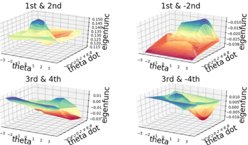
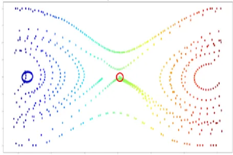
dimensional approximation. In particular, the eigenfunctions of the Koopman operator are approximated using the identified A matrix. The eigenfunctions learned from the neural network can be viewed as intrinsic coordinates for the lifted space and provide insights into the transformed dynamics in the higher dimensional space. An example to illustrate this can be seen in Figure 3.2 and Figure 3.3. These two figures are both 3d plots for eigenfunctions obtained from DNN. The difference is that Figure 3.2 represents a single unforced frictionless pendulum, whereas Figure 3.3 denotes the eigenfunctions obtained for single pendulum under control. As can be seen, the first dominant eigenfunctions from both the two figures exhibit a very similar double-pole structure. The uncovered intrinsic coordinates exhibit a trend that is related to the energy levels within the system as base physical coordinates change, i.e.,θ˙is positively related to the kinetic energy, whereas the θ is proportional to the potential energy. Towards the center of the 3d plot, both kinetic energy and potential energy exhibit declined absolute magnitudes. In the controlled case, torque at the joint is being added into the system’s total energy count, which seeks a path to bring the energy of the system to the maximum in potential energy and lowest absolute value in kinetic energy. Due to the kinetic energy part (1₂θ˙2_{) is dominating the numerical value of the}

energy, this effect has been reflected in the eigenfunction plot corresponding to the 7th and 8th eigenvalue. The two figures show the feasibility of using eigenfunctions from learned Koopman operator to gain insight of the dynamical system, especially for the control purpose.

Then we can proceed to solve discrete LQR problem for the linear system with a quadratic cost:

J(V) =X

t

(35)

Figure 3.2: Eigenfunctions learned from uncontrolled case, Left: real part of eigen-functions, Right: imaginary part of the eigenfunctions. The dominant eigenfunction has zero value imaginary part.

Figure 3.3: Eigenfunctions learned from controlled case, Left: real part of eigenfunc-tions, Right: imaginary part of the eigenfunctions. The dominant eigenfunction has zero value imaginary part.

In case the LQR solution is not sufficient, the method can be easily converted into Model Predictive Control (MPC). For the examples in the Simulation Results section, we used MPC for optimal control due to its flexibility to adjust to problem

(36)

constrains. Given a time horizon of L, we can solve for V ∈_Rm×L _{by minimizing the}

following cost function, as illustrated in Equation 3.8.

J(V) = L−1 X t=0 (z_t>C>QCzt+vt>Rvt) +zL>C > QCzL subject to        vt≤umax−u0 vt≥umin−u0 (3.8)

3.3 Algorithm Summary

To summarize, a schematic diagram of the DKRC framework is shown in Figure 3.4:

The algorithm of Deep Koopman Representation for Control (DKRC) is listed below, where L1(θ) ensures a high dimension linear system, L2(θ) handles the con-trollability of the system:

(37)

System 𝑢 _𝑡

𝑥

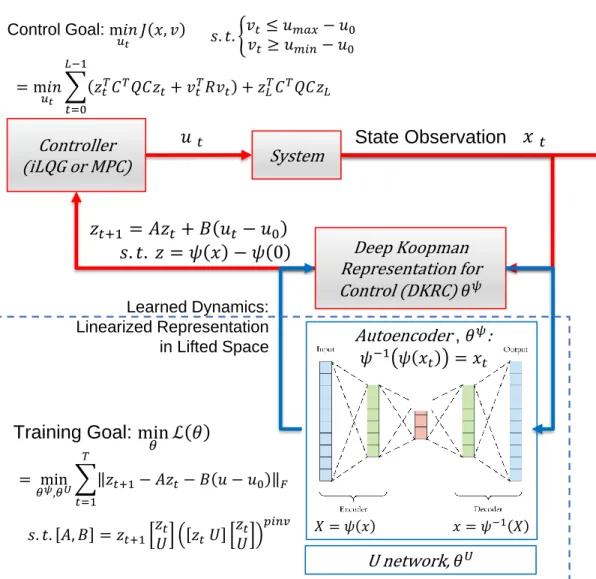
_𝑡 Controller (iLQG or MPC) Deep Koopman Representation for Control (DKRC) 𝜃𝜓 Learned Dynamics: Linearized Representation in Lifted Space 𝑧_𝑡+1 = 𝐴𝑧_𝑡 + 𝐵 𝑢_𝑡− 𝑢₀ 𝑠. 𝑡. 𝑧 = 𝜓 𝑥 − 𝜓 0 State Observation U network, 𝜃𝑈 𝑋 = 𝜓 𝑥 𝑥 = 𝜓−1 _𝑋 Autoencoder, 𝜃𝜓: 𝜓−1 𝜓 𝑥𝑡 = 𝑥𝑡

Training Goal: min

𝜃 ℒ 𝜃 = min 𝜃𝜓_,𝜃𝑈෍ 𝑡=1 𝑇 𝑧𝑡+1− 𝐴𝑧𝑡− 𝐵 𝑢 − 𝑢0 𝐹 𝑠. 𝑡. 𝐴, 𝐵 = 𝑧𝑡+1 𝑧𝑡 𝑈 𝑧𝑡𝑈 𝑧𝑡 𝑈 𝑝𝑖𝑛𝑣 Control Goal: m𝑖𝑛 𝑢𝑡 𝐽 𝑥, 𝑣 = m𝑖𝑛 𝑢𝑡 ෍ 𝑡=0 𝐿−1 𝑧𝑡𝑇𝐶𝑇𝑄𝐶𝑧𝑡+ 𝑣𝑡𝑇𝑅𝑣𝑡 + 𝑧𝐿𝑇𝐶𝑇𝑄𝐶𝑧𝐿 𝑠. 𝑡. ቊ𝑣_𝑣𝑡 ≤ 𝑢𝑚𝑎𝑥− 𝑢0 𝑡 ≥ 𝑢𝑚𝑖𝑛− 𝑢0

(38)

Algorithm 1 Deep Koopman Representation for Control (DKRC)

Input: observations: x, control: u

Output: Planned trajectory and optimal control inputs: (zplan, vplan) • Initialization

1. Set goal position x∗

2. Build Neural Network: ψN(xt;θ)

3. Set z(xt;θ) = ψN(xt;θ)−ψN(x∗;θ) • Steps

1. Set K =z(xt+1;θ)∗z(xt;θ)†

2. Set the first loss function L1 L1(θ) = _L1₋₁PL−1

t=0 kz(xt+1;θ)−K∗z(xt;θ)k

3. Set the second loss function L2 [A, B] =zt+1 zt U zt U zt U † L2(θ) = (N −rank(controllability(A, B))) +||A||1+||B||1

4. Train the neural network, updating the complete loss function

L(θ) =L1(θ) +L2(θ)

5. After converging, We can get system identity matrices A, B, C

C=Xt∗ψN(Xt)†

(39)

Chapter 4 DKRC Implementation Results

In this chapter, we demonstrate the proposed continuous control method based on deep learning and Koopman operator (DKRC) on several example systems offered in OpenAI Gym [3]. The environments considered here are Inverted Pendulum, Cartpole with Double Pendulum, and Lunar Lander (Continuous Control). In this work, we deploy Model Predictive Control (MPC) on Inverted Pendulum, Cartpole with double pendulum, and adopt LQR for Lunar Lander.

The OpenAI Gym utilizes a Box2D physics engine, which provides a dynamic system for the testing. Gravity, object interaction, and physical contact behavior can be specified in the world configuration file. The dynamics of the simulation environment are unknown to the model. The model needs to learn the dynamics through data collected during training. Each simulation game is randomly initialized to generate initial disturbance.

(40)

4.1 Inverted Pendulum

The inverted pendulum environment is a classic 2-dimensional state space environment with one control input, as shown in Equation 4.1.

4.1.1 DKRC solution

A visualization of the simulated environment is also shown in Figure 4.1. The game starts with the pendulum pointing down with a randomized initial disturbance. The goal is to invert the pendulum to its upright position. In order to finish the game, the model need to apply control input to drive the pendulum from start position (θ∈(−π,0)∪(0, π), θ˙= 0) to goal position (θ= 0, θ˙= 0).

Figure 4.1: Inverted Pendulum

χ= [cosθ,sinθ,θ˙] where θ∈[−π, π],θ˙ ∈[−8,8]

U = [u], where u∈[−2,2]

(41)

and sine values to ensure a smooth transition at −π and π. The dynamic governing equation is easy to derive as follows:

ml2θ¨=−γθ˙+mglsin(θ) +u (4.2) This governing equation is unknown to our model, and the model needs to recover the physics-based on limited time-series data only. Moreover, the angular velocity (θ˙) and the torque input (u) at the shaft are also limited to a small range to add difficulties to finish the game. In most of the testing cases, we found that the pendulum needs to learn a swing back-and-forth motion before being able to collect enough momentum from swinging up to the final vertical upright position. Although optimal control is possible, the trained model needs to adapt to the limitation imposed by the testing environment and make decisions solely based on state observations.

Figure 4.2: Trajectories of Swinging Pendulum under Control using trained DDPG reinforcement learning model. The figure exhibits the trajectories of the tip of the pendulum breaking through Hamiltonian energy level lines to arrive at the goal position (θ= 0, θ˙= 0)

(42)

Figure 4.2 shows the trajectory of the pendulum in 2D (θ,θ˙) space based on trained DDPG algorithm. The red circle in the center of Figure 4.2 is the goal position, and the concentric lines on both sides correspond to Hamiltonian total energy levels. It is clear that due to the implicit model learned during the reinforcement learning process, the RL method cannot finish the game within a short time and therefore left many failed trails.

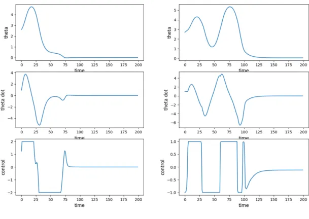
Figure 4.3: Trajectories of Swinging Pendulum under control using DKRC model (left) vs. DDPG RL model (right) initialized at the same state

For comparison between the Reinforcement Learning (DDPG) and DKRC models, we show a single example game in Figure 4.3. The two games were initialized in the same way, and the DKRC model on the left of the figure was able to finish the

(43)

game much cleaner and faster.

Corresponding to the game shown in Figure 4.3, We are also presenting the state vs. time plot for the game played by DKRC model, as shown in Figure 4.4.

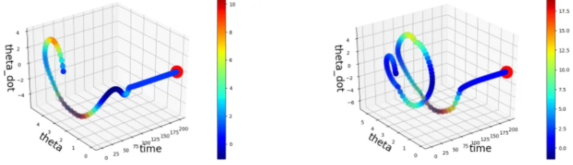
Figure 4.4: Example 3D deployment trajectory from DKRC (left) and Reinforcement Learning (right), colormapped by the magnitude of energy

4.1.2 Stability Test

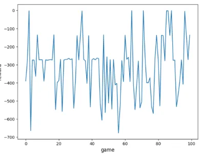
To measure the stability and the performance of the DKRC solution, we run the Swing-up pendulum game for 100 times and record the reward of each game. As defined in the official OpenAi package, the reward for each step is

Reward=−(θ2+ 0.1∗θ˙2+ 0.001∗u2_t)

where reward ∈ [−16.2736044,0], and each game has 200 time steps which means

reward each game∈[−3224,0].The result is shown in Figure 4.5. It can be inferred from the figure that the total reward of each game is different due to different initial positions as expected. Besides, the DKRC has a 98%successful percentage for 100 games.

(44)

Figure 4.5: 100 games recorded reward using DKRC

4.2 Acrobot

Acrobot is another classic control scenario. We swing a double pendulum with only one actuation at the joint between the two links, which simulates the swing up motion of a human acrobat. Initially, both links point downwards (initial sweeping angles are zero to the world coordinate system). The two links are allowed to swing in any direction at the two joints, without any collision if they are with the same sweep angle. The goal is to swing the end-effector at a height at least the length of one link above the base. The same simulation has been performed mainly for reinforcement learning algorithm developments [36]. A schematic of the environment setup is shown in Figure 4.6

The state consists of the two rotational joint angles and their velocities: [θ1, θ2, θ1˙ , θ2˙]. For the same consideration in the inverted pendulum case, to ensure numerical smoothness during transition from−π andπ, we use the following

(45)

state-Figure 4.6: Acrobot ¨ θ1 =−d−11(d2θ¨2+φ1) ¨ θ2 = (m2lc22 +I2− d2₂ d1 )−1(τ + d2 d1 φ1−m2l1lc2θ˙ 2 1sinθ2−φ2) d1 =m1l2c1 +m2(l 2 1+l 2 c2 + 2l1lc2θ˙ 2 1sinθ2−φ2) +I1+I2 d2 =m2(l2₁+l_c2₂ + 2l1lc2θ˙ 2 1sinθ2−φ2) +I2 φ1 =−m2l1lc2θ˙2 2 sinθ2−2m2l1lc2θ˙2θ˙1sinθ2 +(m1lc1+m2l1)gcos θ1− π 2 +φ2 φ2 =m2lc2gcos θ1+θ2− π 2

(46)

If we want to make θ1 = π/2, θ2 =−π/2,θ˙1 = ˙θ2 = 0as equilibrium point, this

will require making θ¨1 = ¨θ2 = 0 and hence we have φ?₂ = 0

φ?₁ = (m1lc1 +m2l1)g

4.2.1 DKRC solution

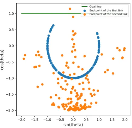
Here, to take advantage of our MPC controller optimized for continuous control, we customized the environment to use continuous torque at the joint, instead of the OpenAI default discrete input [-1, 0, 1] for the torque. The trajectory of the two links are shown in Figure 4.7. We can finish the game every time according to the criteria listed on the OpenAI leaderboard, as shown in Figure 4.7.

4.2.2 Stability Test

Again, to measure the stability and the performance of the DKRC solution, we run the Acrobot game for 100 times and record the total reward of each game. As defined in the official OpenAi package, the reward for each step is

reward=−1, if not terminal else0

which means rewardeachgame∈[−400,0].The result is shown in Figure 4.8. It can be inferred from the figure that the total reward of each game is different due to different initial positions as expected. Besides, the DKRC has a 97% successful percentage for 100 games in this scenario.

(47)

Figure 4.7: DKRC deployment trajectories of Acrobot under Control. As shown in the picture, the green line is goal line for second link.The goal of this game is to touch the green line with the second link

4.3 Double Pendulum on a Cart

A schematic of the double pendulum on a cart environment is shown in Figure 4.9. This testing case is carried out in a customized OpenAI environment that combines two existing OpenAI Gym environments "cartpole" and "acrobot" in one simulation. In this case, a double pendulum is attached to a cart by an un-actuated joint. The cart moves along a frictionless track and can be driven by force in the horizontal direction. The two links of the double pendulum can swing independently without any friction or collision. The pendulum starts upright with a randomized initial disturbance. The

(48)

Figure 4.9: Cartpole with double pendulum

goal is to prevent it from falling over by applying force to the cart in the horizontal direction. We use the following state-space observations for training.

χ= [x, θ1, θ2,x,˙ θ˙1,θ˙2]

(49)

4.3.1 DKRC solution

Figure 4.10: Balance keeping process for one game using DKRC

The control input is being applied to the cart and then translated to the motion of the two links. The state measurements of two links are depicted in Figure 4.10. As can be seen in the figure, both the two swing angles (θ1,θ2) and corresponding angular

velocities (θ˙1, θ˙2) are kept within a tight range (axis zoomed-in to show the trend).

The state observables oscillate around a value close to 0 throughout the testing period (end of steps), which means that the learned model can maintain a dynamic balance

(50)

4.3.2 Stability Test

To measure the stability and performance of the DKRC solution, we run the Swing-up pendulum game for 100 times and record each game’s reward. As defined in the official OpenAi package, the reward for each step is

Reward =−(θ₁2+θ₂2)

The result is shown in Figure 4.11. It can be inferred from the figure that the maximum

reward of this game is 0, and the DKRC has a 97% successful percentage for 100 games.

4.4 Lunar Lander

As depicted in Figure 4.12, the lunar lander environment is a 6-dimensional state space with 2 control inputs. The state observables involve more terms and

(51)

examples.

χ= [x, y, θ,x,˙ y,˙ θ˙]

U = [u1, u2], where, u1 ∈[0,1], u2 ∈[−1,1]

(4.4) where x,y are the Cartesian coordinates of the lunar lander, and θ is the orientation angle measured clockwise from the upright position. u1 represents the main engine on

the lunar lander, which only takes positive input. In contrast, the u2 is the side engine

that can take both negative (left engine firing) and positive (right engine firing) values. The goal of this game is to move lunar lander from initial position (x= 10, y= 13) to the landing zone (x= 10, y= 4), subject to randomized initial gust disturbance and dynamics specified in the Box2D environment.

Figure 4.12: Lunar Lander

The exact model for this system cannot be extracted directly from the OpenAI Gym environment but has to be identified either through a data-driven model-based approach (this paper) or model-free approach (e.g., reinforcement learning). A game score is calculated by OpenAI Gym where the system will reward smooth landing within the landing zone (area in between double flags) while penalizing the fuel consumption by engines (U). The proposed method is then to generate the model of

(52)

system identification. Assuming after the Koopman operator transform, the dynamical system can be considered to be linear. Therefore, model predictive control can be applied. The trajectories of the lunar lander successfully finishing the game are shown in Figure 4.13. Note that the trajectories for the ten games are spread out in the simulation environment and returning back to the same goal position. The reason for the spread-out behavior is that the initialization of each game will randommly assign an initial velocity and the control algorithm need to apply control to offset the drift while keeping balance in the air. In this simulation environment, the DKRC model was demonstrated to be able to learn the dynamics and cope with the unforeseen situation using Model Predictive Control.

Figure 4.13: DKRC deployment for ten games, Red point: starting point, Blue point: goal position

(53)

Figure 4.14: Data visualization of the training sample for Lunar Lander environment. The 1876 data pairs are obtained from playing five games. The different color gradient represents different state observations and control inputs collected. Each row on Left figure denotes one of six states; right figure shows the control input from main and side engine thrusts

4.4.1 DKRC solution

The data collection can be obtained by running a reinforcement learning algorithm with random policy together with a random noise generated by the Orn-stein–Uhlenbeck process during the data collection procedure. These randomization treatments are implemented to ensure enough exploration vs. exploitation ratio from the Reinforcement Learning model. A sample visualization of the collected data is shown in Figure 4.14 to demonstrate how few amounts of data are needed to train the proposed learning algorithm, which poses a significant advantage compared to state-of-art reinforcement learning methods.

(54)

4.5 Experiment Conclusion

In this first part of the thesis, we propose MPC controller designed by Deep Koopman Representation for Control (DKRC) has the benefit of being completely data-driven in learning, whereas it remains to be model-based in control design. The DKRC model is efficient in training and sufficient in the deployment in four OpenAI Gym environments compared to a state-of-the-art Reinforcement Learning algorithm (DDPG).

(55)

Chapter 5 Data Driven Control: Model-based vs.

Model-free Approach

In this chapter, we compare the proposed DKRC algorithm with another classic model-free control method – Deep Deterministic Policy Gradient (DDPG), in terms of the algorithm control strategies, robustness, and the learned dynamics of DKRC with the classic Euler-Lagrange Linearization method to validate the learning efficiency of DKRC.

5.1 Experiment Setup

To obtain benchmark comparison results, we use the classic ’Pendulum-v0’ OpenAI Gym environment [3] to examine the behaviors of controllers built based on DDPG and DKRC for this inverted pendulum problem. The OpenAI Gym is a toolkit designed for developing and comparing reinforcement learning [35]. The inverted pendulum swing-up problem is a classic problem in the control literature, and the goal of the system is to swing the pendulum up and make it stay upright, as depicted

(56)

in Figure 5.1. Although both the two approaches are data-driven in nature, thus versatile in deployment, We would like to still stick with the classic control problem, which has rich documentation of analytical solution for later comparisons. As shown in the next section, the DKRC approach successfully finishes the control task using a learned dynamics that directly resembles the analytical solution and can also explain the system in lifted dimensions using Hamiltonian Energy Level theorem.

Figure 5.1: Environment visualization

5.1.1 Problem set-up

A visualization of the simulation environment is shown in Figure 4.9. As shown in the picture, the simple system has two states x= [θ,θ˙] and one continuous control moment at the joint, which numerically must satisfy−2≤u≤2. This limit in control magnitude is applied with the intention to add difficulty in designing the control strategy. For the default physical parameter setup, the maximum moment that is

(57)

the upright position in one single move. The control strategy needs to learn how to build momentum by switching moment direction at the right time. The OpenAI Gym defines the observations and control in Equation 5.1.

χ= [cosθ,sinθ,θ˙], where θ∈[−π, π],θ˙∈[−8,8]

U = [u], where u∈[−2,2]

(5.1) The cost function is designed in Equation 5.2. The cost function tracks the current states (θ) and control input (u). The environment also limits the rotational speed of the up-swing motion, by including a θ˙2 _{term in the cost function. By minimizing this}

cost function, we ask for the minimum control input to ensure the pendulum ends at the upright position with minimum kinetic energy levels. During the comparison, we are using the Equation 5.2 directly in the controller design for the DKRC, whereas we negate cost function and transforms it into a negative reward function, where 0 is the highest reward for the DDPG training. By using this simple simulation environment, we ensure the two approaches are being compared on the same basis with the same reward/cost function definition.

reward=θ2 + 0.1 ˙θ2+ 0.001u2 (5.2)

The dynamical system of the swing-up pendulum can be analytically solved by Euler–Lagrange method [14], with its governing equation shown in Equation 5.3, where θ= 0 is the upright position, g is the gravitational acceleration,m is the mass of the pendulum, l is the length of the pendulum.

¨

θ =−3g

2l sin(θ+π) + 3

(58)

By converting the second order ordinary differential equation(ODE) in Equation 5.3 to the first order ODE, we can get Equation 5.4.

d dt       cosθ sinθ ˙ θ       =       0 −1 0 1 0 0 0 3₂g_l 0             cosθ sinθ ˙ θ       +       0 0 3 ml2       u (5.4) We use the default physical parameters defined in the OpenAI Gym, i.e., m= 1,l = 1,

g = 10.0,dt = 0.05. We discretize the model using zero order hold (ZOH) method [12] with a sampling perioddt. As a result, we can achieve the linearized governing Equation 5.5 with observed statesyt. The numerical values for the hyperparameters used in the

default problem setting are also listed in Equation 5.6. Also one predictive result is that Euler-Lagrange method only works between a small initial angle assumption as a result of sinθ =θ, cosθ= 1 is validate under small angle assumption.

xt+1 =Adxt+Bdut yt =Cxt (5.5) with Ad=       0.9988 −0.04998 0 0.04998 0.9988 0.05 0.01875 0.7497 1       Bd=       0 0 0.15       C =       1 0 0 0 1 0 0 0 1       (5.6)

(59)

We use Ad and Bd as the benchmark of learned dynamic models comparison between

DKRC and Euler-Lagrange Linearization in later sections.

5.1.2 Parameters of DDPG and DKRC

The following Table (5.1) is the parameters we use to obtain DDPG and DKRC solutions. Both two methods are trained on NVIDIA Tesla V-100 GPUs on an NVIDIA-DGX2 supercomputer cluster.

Table 5.1: Parameters of different methods Method Parameter Value

Buffer size 1e6 Batch size 64

γ (Discount factor) 0.9 DDPG τ (Target Network Update rate) 0.001

Target & Actor learning rate 1e-3 Target & Critic learning rate 1e-2 Training epochs 5e4 DKRC Lift dimension 8

Training epochs 70

The result of the DDPG solution is an Actor neural network with optimal parameters for the nonlinear pendulum system - µ(x;θ∗).

The result of the DKRC solution is identity matricesAlif t,Blif t,C of the lifted

space, and a lift neural network ψN(x;θ) for observations of the unknown dynamical

system.

5.2 Control Strategies of DDPG and DKRC

We present results from the DKRC vs DDPG by specifying five initialization configuration for the problem. We have choices of defining the starting position and

(60)

also the initial disturbance in the form of starting angular velocity of the pendulum. In this study, we initialize the pendulum at five different positions: θ0 = π (lowest

position), θ0 = π₂ (left horizontal position), θ0 = −π₂ (right horizontal position), θ0 = ±₁₈π (close to upright position). The initial angular velocity of pendulum at

different initial positions is θ˙0 = 1rad/s (clockwise). For better visualization, we map

the angle from [−π, π] to[0,2π], where the upright position (goal position) is always achieved at θ = 0 and θ˙= 0. The result is shown in Figure 5.2− 5.5.

Figure 5.2: Trajectories of Swinging Pendulum implementing DDPG model (left) vs. DKRC model (right) initialized at the lowest position

Figure 5.2−5.6 show that DDPG and DKRC have similar control strategies in most initial positions. DDPG needs less time to arrive at the goal position than DKRC when the pendulum is initialized on the right side. It tends to use smaller control torque as a result of that DDPG has constraints term for control torque. Still, DDPG never succeeds in getting an absolute upright position, i.e., at the final position, a non-zero control input is always required to sustain a small displacement away from

(61)

Figure 5.3: Trajectories of Swinging Pendulum implementing DDPG model (left) vs. DKRC model (right) initialized at the left horizontal position

Figure 5.4: Trajectories of Swinging Pendulum implementing DDPG model (left) vs. DKRC model (right) initialized at the right horizontal position

(62)

Figure 5.5: Trajectories of Swinging Pendulum implementing DDPG model (left) vs. DKRC model (right) initialized at the close left upright position

Figure 5.6: Trajectories of Swinging Pendulum implementing DDPG model (left) vs. DKRC model (right) initialized at the close right upright position

(63)

much less training time than DDPG. Once a proper dynamical system model can be learned directly from data, it makes more sense to execute control using model-based controller design such as MPC.

Another way to show the differences in control strategies is by plotting the measured trajectories during repeated tests. In Figure 5.7, we test the pendulum game for 50 games with a total of 10000 time-steps utilizing both methods (DDPG & DKRC) solutions. In this comparison, we plot the measurements ofθ˙ vs. θ on a 2D

Figure 5.7: 50 pendulum games data recorded using DDPG model (left) vs. DKRC model (right), color mapped by energy

basis, colored by the magnitude of the cost function defined in Equation 5.2. The goal is to arrive at the goal position (θ˙= 0 and θ = 0, the center of each plot) as quickly as possible. Figure 5.7 shows that DDPG tends to drive the states into "pre-designed" patterns, and execute similar control strategies for the 50 games. Therefore the data points on the left subplot appear to be less than the one on the right. DKRC, on the other hand, tends to exhibit different control behavior due to the local replanning using MPC. The result of the local replanning is that it generates multiple trajectories

(64)

solving the 50 games with different random initializations. During this comparison, we illustrate that DDPG is indeed deterministic, which is a good indicator of the system’s reliability. However, we want to point out that the robustness of the system will also benefit from a local replanner available under different initializations or disturbances since the "pre-designed" patterns are learned from past experience, therefore, cannot guarantee a viable solution for unforeseeable situations when we move onto more complex systems.

By transforming the observed states, we can also show the relationship between the designed control and the energy levels in the system. Consequently, our control goal is to achieve the lowest energy level of the system in terms of lowest magnitudes in both kinetic energy and potential energy. In Figure 5.8, we present the Hamiltonian energy level plots with respect to the measured states (θ,cos(θ),sin(θ), andθ˙) for the forced frictionless pendulum system, each colored by the same energy level scale. The energy term used in forced pendulum is defined as 1₂θ˙2₊_cos₍_θ_{) +}_u_{. Figure 5.8 shows}

Data-Driven Control with Learned Dynamics

TigerPrints

TigerPrints

Data-Driven Control with Learned Dynamics

Data-Driven Control with Learned Dynamics

Data Driven Control with Learned Dynamics

Acknowledgments

Abstract

Table of Contents

List of Tables

List of Figures

Chapter 1

Introduction

1.1

Koopman Operator

1.2

Model Predictive Control

1.3

Reinforcement Learning

1.3.1

Deep Deterministic Policy Gradient

1.4

Thesis Organization

Chapter 2

Research Problem Setup

2.1

Problem Set-up

2.2

Proposed Solutions

2.2.1

The First Solution

2.2.2

The Second Solution

2.3

Lessons Learned

Chapter 3

Algorithm Proposed

3.1

Deep Learning of Koopman Representation for

Control

…

…

…

…

…

…

…

…

…

3.2

Koopman-based Control

3.3

Algorithm Summary

𝑥

Chapter 4

DKRC Implementation Results

4.1

Inverted Pendulum

4.1.1

DKRC solution

4.1.2

Stability Test

4.2

Acrobot

4.2.1

DKRC solution

4.2.2

Stability Test

4.3

Double Pendulum on a Cart

4.3.1

DKRC solution

4.3.2

Stability Test

4.4

Lunar Lander

4.4.1

DKRC solution

4.5

Experiment Conclusion