Procedia Computer Science 58 ( 2015 ) 66 – 75
1877-0509 © 2015 The Authors. Published by Elsevier B.V. This is an open access article under the CC BY-NC-ND license (http://creativecommons.org/licenses/by-nc-nd/4.0/).
Peer-review under responsibility of organizing committee of the Second International Symposium on Computer Vision and the Internet (VisionNet’15) doi: 10.1016/j.procs.2015.08.014
ScienceDirect
Second International Symposium on Computer Vision and the Internet (VisionNet’15)
A
ffi
ne Normalized Krawtchouk Moments based Face Recognition
B. H. Shekar, D. S. Rajesh
∗Department of Computer Science, Mangalore University, Mangalaaangothri, Mangalore, India
Abstract
In this paper, we have developed a new local descriptor based on Krawtchouk polynomial moments. The interest points are initially detected using the Canny edge detector and made the region around each interest point scale and affine normalized. The region is then represented using Krawtchouk polynomial and hence formed the descriptor. Experiments have been conducted keeping the face recognition problem in focus. By using the sparse representation concept, classification of face images is done. Experimental results on the ORL dataset and a subset of pose and illumination variant FERET dataset have shown the classification capability of our descriptor for face recognition applications.
c
2015 The Authors. Published by Elsevier B.V.
Peer-review under responsibility of organizing committee of the Second International Symposium on Computer Vision and the Internet (VisionNet’15).
Keywords: Krawtchouk polynomials, Krawtchouk moments matrix, Sparse representation, Face recognition.
1. Introduction
We have seen works being carried out in the field of biometrics to provide security to information access. Among many biometric traits, face is considered as one of the major biometric. Although it is quite feasible to access face im-ages, one needs to address many challenging problems such as face occlusion, blurry image, poor illumination, both non-linear (like affine viewpoint) and linear (like in plane and offplane rotations) transformations of face images, ageing etc. To efficiently handle these challenges, researchers have come up with robust algorithms to extract facial feature as well as several mathematical models for preprocessing such features for better classification. However, designing an efficient/accurate face recognition system is still a complex problem.
We have seen many solutions to face representation/recognition in both frequency domain and spatial domain. The global descriptors found to work well in case of faces posing front, but fails in handling occlusion and pose variations and hence the local descriptors are commonly used to address many of the challenges in face recognition. Among many of the approaches, Gabor transform is extensively used for face recognition. The Gabor transform, which re-sembles the cortical cell response of vision in mammals has been used with significant success in many biometric applications such as1where they down sampled the Gabor responses (of 5 scales and 8 orientations) of the face
im-age to remove redundancy during feature representation and used sparse representation based classification for face
∗Corresponding author. Tel.:+91-9448625976
E-mail address:[email protected]
© 2015 The Authors. Published by Elsevier B.V. This is an open access article under the CC BY-NC-ND license (http://creativecommons.org/licenses/by-nc-nd/4.0/).
Peer-review under responsibility of organizing committee of the Second International Symposium on Computer Vision and the Internet (VisionNet’15)
recognition. They used the occlusion dictionary to handle the occlusion problem. Liao et al.2used the Gabor Ternary
Pattern (GTP) to represent the scale and affine normalized regions around interest points of a face image. They con-solidated the Gabor responses corresponding to four different orientations in a single Gabor pattern. Recently, Li et al.3used a 2D histogram of differential excitation (based on Weber’s law) versus orientation to represent face images.
Dabbaghchian et al.4proposed DCT based approach for face recognition. Vidya et al5proposed Discrete Wavelet
Transform approach in which poorly illuminated areas of the face were selectively enhanced using an energy function based correction factor to increase the discriminative capability of the descriptor.
On the other hand, many orthogonal polynomials in computer vision domain have been reported for image reconstruc-tion purpose. Mukundan et al.6demonstrated the reconstruction capabilities of Tchebichef orthogonal polynomials
through reconstruction of English and Chinese letter images. Jassim et al.7derived a new set of orthogonal
polyno-mials from the Krawtchouk polynomial and Tchebichef polynopolyno-mials. Using this new set of orthogonal polynomial moments matrix, they demonstrated its reconstruction capabilities on various real world images. Yap et al.8
demon-strated the reconstruction capabilities of Krawtchouk orthogonal polynomials moments matrix through reconstruction of English letter and other images. Based on the krawtchouk moments matrix they suggested the use of image recon-struction errors for classification. Observing the excellent image reconrecon-struction capabilities of Krawtchouk moments matrix, we are motivated to explore the capabilities of Krawtchouk moments for face recognition problem. The re-maining part of the paper is organized as follows. In Section 2, we discuss the basics of Krawtchouk polynomials and its parameters. The affine viewpoint and scale normalization method is given in Section 3. In Section 4, we discuss in detail about how sparse representation is used in classification. Experimental results on ORL and a subset of FERET face dataset is given in Section 5. Conclusion is presented in Section 6.
2. Krawtchouk moments based face recognition 2.1. Krawtchouk moments
Let X be the discrete point in n dimensional space. The Krawtchouk polynomials of order ’n+1’ at a point ’x’ can be generated by the recurrence relation:9
Kn(p+)1(x,X)= X p−2np+n−x (X−n)p ∗K (p) n (x,X)− n(1−p) (X−n)p∗K (p) n−1(x,X) (1)
withK1(p)(x,X)=1−X px andK0(p)(x,X)=1 , ’p’ being the shift operator which controls the shift of the polynomial. These polynomials form the Krawtchouk basis polynomial functions satisfying the orthogonality condition.
X
x=0
ω(p)(
x,X)Kn(p)(x,X)Km(p)(x,X)=ρ(p)(n,X)δnm (2)
where n,m=1,2,. . .,X andδnmbeing the Kronecker impulse function,ωbeing the weight function
ω(p)( x,X)= X x px(1−p)X−x (3) and ρ(p)(n,X)= 1−p p n 1 X n (4)
The reasons for using a value of 0.5 for ’p’ are:
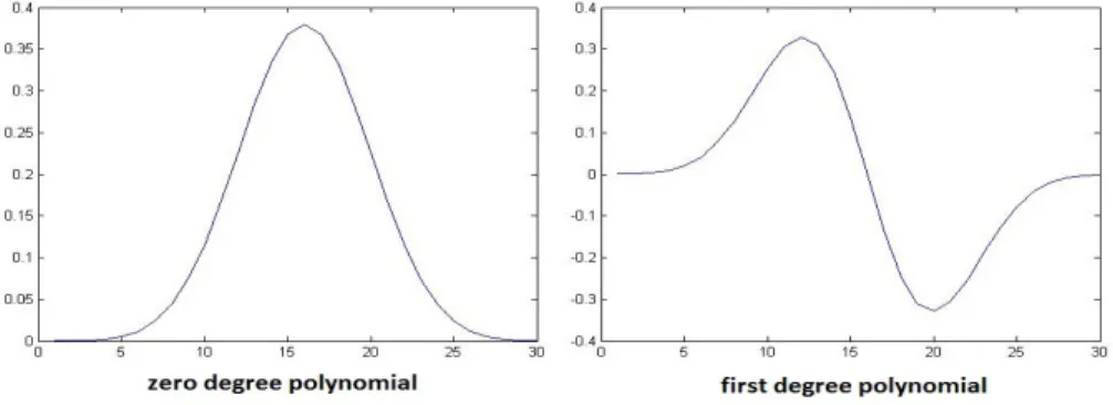
• We have used Krawtchouk polynomials to describe affine normalized regions around interest points. ’p’ can take values between 0 and 1. The lower order polynomials will concentrate more in extracting features at the center (polynomials have a peak at the center see fig.2) of the region around interest points (i.e that part of the region where interest point lies) if we use a value of p=0.5. For us details around the center are more important
Fig. 1. The affine normalization procedure.
(only then the description will be pose and rotation invariant) than the details away from it. If we use values other than 0.5 the lower order polynomials shown in fig.2 and 3 will be not symmetric and their peak will shift either to the left or right depending on the value of ’p’ being>0.5 or<0.5 respectively. Hence their concentra-tion diverts away from the center of the region around interest points during feature representaconcentra-tion.
• The second reason for assigning a value of 0.5 for ’p’ is that it will reduce a lot of derivational and computational effort in moment calculation (eq.1). Even with a value of p=0.5, as we proceed to compute the higher order polynomials (recurrence relations mentioned in eq.1) the computation time grows exponentially. On a 3.3GHz I3 4GB machine it takes around two hours for the degree 29 polynomial (fig.3) computation and the higher order polynomial computation may take days. Also this is the reason why we stop polynomial computation at degree 29 (degree 0 to degree 29) totalling upto 30 order polynomials and hence the size of the interest point region is scaled down/up to 30x30. Moreover the polynomials till degree 29 are sufficient for feature representation as our experimental results show.
The expression for the normalized and weighted Krawtchouk polynomials is given by
Kn (p) (x,X)=Kn(p)(x,X) ω(p)(x,X) ρ(p)(n,X) (5)
. This weighting and normalization operation controls stability and numerical fluctuations of these polynomials during moment computation8. The Krawtchouk moment matrixQof a X x X image I(i,j) is given by:
Q=KAKT (6) whereQ = Qji i,j=X−1 i,j=0 K = Ki(j,X−1) i,j=X−1 i,j=0 A ={I(j,i)} i,j=X−1
i,j=0 . Kis obtained by stacking all the 30 point
discrete polynomials upto order 30 one below the other to form a matrix. In our work we use the difference between the probe image descriptor moment matrix and the gallery image descriptor moment matrix as the measurement criteria for classification.
3. Affine and scale normalized descriptors
Affine viewpoint transformation is a non-linear transformation occurring when two images ’a’ and ’b’ of the same scene are captured from different angles. Under this transformation, the region around any interest point in image ’a’ and the region around the same interest point in image ’b’ will have different pixel distribution (the principal eigen values of pixel intensity variation around these two interest points will not be the same). Hence any interest point based matching algorithm will infer incorrectly that these two same regions of images of the same scene are different even though they are same. Hence all such transformed regions will not cooperate in the matching process
Fig. 2. The degree 0 and degree 1 normalized weighted Krawtchouk polynomials.
Fig. 3. The degree 2 and degree 29 normalized weighted Krawtchouk polynomials.
and increase the misclassification rate unnecessarily. Mikolajczyk et al10came up with the technique of scale and
affine normalization of such image regions. Here the region around any interest point is normalized in such a way that the principal eigen values of pixel intensity variation around this interest point will be same (the ratio of the two principal eigen values is 1). Hence the region around any interest point in image ’a’ and the region around the same interest point in image ’b’ will be identical (because the principal eigen values of pixel intensity variation around these same interest points will be the same due to the scale and affine normalization process). Hence these affine transformed regions will regain the capacity to cooperate in proper matching and the misclassification rate can be reduced considerably. This technique has helped many researchers in obtaining descriptors which are robust against affine viewpoint transformation. In our work, we have used the same technique to handle variations in face image features due to affine viewpoint transformation i.e., due to pose and expression variation. We use the scale invariant Canny edge based interest point detector used by Liao et al.2to extract interest points from face images. We use the
software provided in11for this purpose. A square region around each interest point is scale and affine normalized and
this process in illustrated in Fig. 1. This square region around the affine normalized interest point (whose area depends on the scale of the affine normalized interest point) is resized to 30x30 pixels. Thus, around each of the interest point an affine normalized pixel region is formed from which a descriptor is created using Krawtchouk moments as follows. By using Eq. 6 we compute the moment matrix (of 30x30 size) of this region which forms our Krawtchouk polynomial moments based descriptor. A few among the 30 Krawtchouk polynomials used to compute the Krawtchouk moment matrix and generated by us are shown in Fig. 2 and Fig. 3.
4. Sparse representation based classification
Suppose we have a library of frontal face images of ’S’ subjects withn1,n2,n3....nS being respectively the number
of face images belonging to subject 1, subject 2....subject S. According to sparse representation based face recogni-tion12, any frontal test face image ’t’ is representable as the linear sum of all the library face images i.e
t=Aα (7)
whereA=A1,A2, ....AS withA1,A2, ...AS being the face images belonging to subject 1,2....S respectively. The above
problem can be formulated as a minimization problem solved by L1-minimization technique i.e.,
α=argmin
αt−Aα22+λα1 (8)
whereα=α1, α2....αSbeing the coefficients corresponding to subjects 1,2....S respectively obtained during the above
minimization (Eq. 8). AlsoA1 = A11,A12,A31...An11 whereA11,A21,A13...An11 aren1 number of subject-1 face images, A2=A12,A22,A32...An22whereA12,A22,A32...An22aren2number of subject-2 face images andAS =A1S,A2S,A3S...A
nS S where A1
S,A2S,A3S...A nS
S arenS number of subject-S face images. Alsoα1 =α11, α21....αn11being the linear coefficients
corre-sponding to each ofn1face images of subject-1 andαS =α1S, α2S....α nS
S being the linear coefficients corresponding
to each ofnS face images of subject-S obtained during the above minimization (Eq. 8). If the test face belongs to
say class- 1, exceptα1 =α11, α21....αn11all other coefficients will have a value nearly equal to zero and if the test face
belongs to say class 2, exceptα2=α12, α22....αn22all other coefficients will have a value nearly equal to zero and so on.
Using these coefficients and library face images for reconstruction of the test image, classification of the test image is done as explained next.
• Firstly, the test image is reconstructed using coefficients (α1 = α11, α21....αn11) and images of subject 1 (A1 = A1 1,A 2 1,A 3 1...A n1
1) only and then the test image is reconstructed using coefficients (α2=α 1 2, α 2 2....α n2 2) and images
of subject 2 (A2=A12,A22,A32...An22) only and so on.
• In each case the reconstruction error between the test image and the reconstructed test image is computed and that subject using whose images the reconstruction error is found to be minimum is declared as the subject of the test image.
For example the reconstruction error between the test image and the reconstructed test image using library images of subject ’i’ is computed as follows:
errori=t−Aiδi
α2 (9)
whereδiis a function which sets all the coefficients ofα
except the ones that belong to subject ’i’ to zero andAi
being the images belonging to subject ’i’. This is how sparse representation concept is used in classification in face recognition12. In our work we use sparse representation concept at the descriptor level instead of using the full face for classification. We use all the descriptors of the test face (obtained by the method explained in section 2.2) in the classification process as follows. Descriptors of all library faces are pooled together to form descriptor library L. Let
Ld1=Ld11,Ld21...Ld n1
1 be then1number of descriptors of all subject-1 faces pooled together, wheren1stands for the
number of descriptors belonging to subject-1 facesA1, letLd2=Ld21,Ld22...Ld n2
2 be then2number of descriptors of all
subject-2 faces pooled together and so on. Lettd=td1,td2...tdntbe then
tnumber of all descriptors of test face. Each
of thesentdescriptors takes part in decision making as explained below. Any jthtest face descriptortdjis sparsely
represented with respect to library of descriptors L:
α=argmin
αtdj−Lα22+λα1 (10)
At first reconstruction of this descriptortdjis done using library descriptorsLd
1of subject 1 and its coefficients only
and then using library descriptors of subject 2Ld2only and its coefficients only and so on. For example reconstruction
error computation oftdjwith respect to subject ’i’error
iis done as follows: errori=tdj−Ldiδi
Table 1. Recognition rate of the proposed method for ORL face dataset with varying no. of training samples.
No. of training samples Recognition rate
3:7 97.86%
4:6 98.33%
5:5 99.00%
Table 2. Recognition rate of different methods for ORL face dataset with 3:7 training to testing sample ratio.
Method Recognition rate
ThBPSO14 95.00%
SLGS15 78.00%
KLDA16 92.92%
NNRW17 89.80%
2D-NNRW18 91.90%
The proposed method 97.86%
whereδiis a function which sets to zero all the coefficients inα except that belonging to subject ’i’ andLdi are
the descriptors belonging to subject ’i’ face. The test descriptortdj belongs to that subject with respect to whom
the reconstruction error is the least and the descriptor will vote in favour of that subject. In the same way each test descriptor is made to vote to the nearest subject with respect to whom its reconstruction error is minimum. The test face belongs to that subject who gets the maximum of votes like this from among the votes cast by all the descriptors of test face.
5. Experimental Results
This section presents the results of the experiments conducted on the pose, illumination and expression variant face datasets to demonstrate the performance of the proposed approach. Our work is based on affine viewpoint and scale normalized regions around interest points. Hence, we have selected datasets which offer challenges like pose and expression variation.We have considered the ORL dataset and a subset of the FERET dataset. In FERET we have selected 6 images per subject such that each image is different in pose compared to the other images of the same subject. All experiments were performed on a I-3, 3.30GHz Windows machine with 4GB of RAM.
5.1. Experimentation on ORL Dataset13
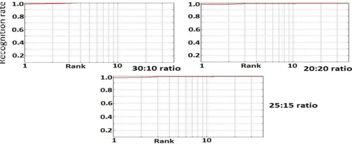
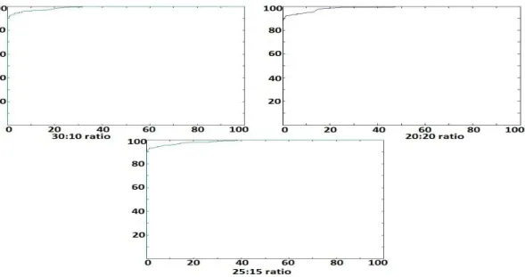
The ORL face dataset contains 10 face images of each of the 40 subjects captured over a period of time with varying pose, expression and illumination. In order to demonstrate the effectiveness of Krawtchouk moment based descriptors we have carried out experiments by varying the training to testing ratios like 3:7, 4:6 and 5:5. The results of these experiments are shown in Table 1. The cumulative match score of the proposed method for various training to testing sample ratios are shown in fig.4. The CMC curves indicate a high recognition rate even at rank 1. The ROC curve drawn for various client to imposter ratios are shown in Fig. 5, Fig. 6 and Fig. 7 which indicate the high genuine acceptance rate even under low false acceptance rate indicating the accuracy of the proposed approach. The comparative analysis results are shown in Table 2. We can see that the proposed approach has performed well compared to many other contemporary works. With just 3 samples per subject for training, we obtained a recognition rate of 97.86%.
5.2. Experimentation on FERET dataset19
The FERET database contains 14,126 images from 1199 individuals. The images show variation in pose, expres-sion, illumination and ageing effect. In our experiments, we chose 200 subjects with 7 images per subject taken on different dates (varying from few days to 2 years). The selected images show variation in illumination, expression and pose. Also images of each subject show variation in facial features (because images were captured over a period of
Fig. 4. The Cumulative match score curve of the proposed method for ORL face dataset with varying number of training to testing samples ratio
Fig. 5. The ROC curve of the proposed method with 5:5 training to testing ratio for ORL face dataset with varying number of client to imposter ratios.
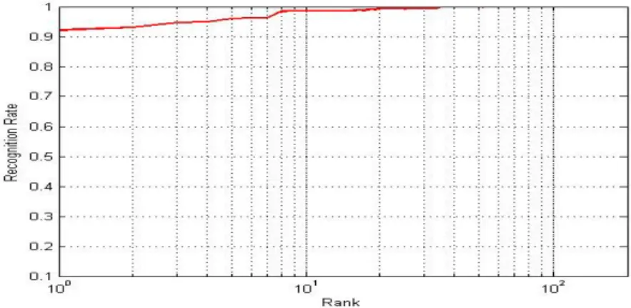
few days to 2 years). In our experiments, to plot the CMC curve we have randomly selected three images per subject for training and the rest for testing( i.e 600 images for training and 800 images for testing totally). The proposed method showed a recognition rate of 91.25%. We have also made a comparative study with some of the recently pro-posed methods and the results are shown in Table3. Due to the scale and affine viewpoint normalization that we have used our results are well above the performance of the state of the art works mentioned in the table. Fig.8 shows the CMC (cumulative match score) curve performance of the proposed method. The ROC curve shown in fig.9 shows the performance of the proposed method on face recognition. For plotting the ROC curve, experiment was conducted with 150:50 client to imposter ratio. That is out of the 200 subject images, 150 subject images (i.e 150x7=1050 images) were broken into 450 gallery images and 600 client testing images, while the remaining 50 subject images (50x7=350 images) were used as imposter testing images. Also the ratio of training to client testing samples ratio was fixed to 3:4 ratio (i.e 450 gallery images (150x3) and 600 client testing images (150x4) as mentioned above). The imposter images belonging to the 50 subjects never appeared in the gallery.
Fig. 6. The ROC curve of the proposed method with 4:6 training to testing ratio for ORL face dataset with varying number of client to imposter ratios.
Fig. 7. The ROC curve of the proposed method with 3:7 training to testing ratio for ORL face dataset with varying no. of client to imposter ratios (mentioned below each curve).
Table 3. Recognition rate of different methods for FERET face dataset with 3:4 training to testing sample ratio
Method Recognition rate
PCA20 42.25% LDA20 45.50%
KLDA16 52.63%
IFDA21 51.25%
KPCA22 43.50% The proposed method 91.25%
Fig. 8. CMC curve of the proposed method for FERET face dataset with 3:4 training to testing samples ratio.
Fig. 9. ROC curve of the proposed method for FERET face dataset with 3:4 training to testing samples ratio and 150:50 client to imposter subject ratio (600:350).
6. Conclusion
In this paper, we explored the use of Krawtchouk moment matrix for face recognition, which has shown excellent image reconstruction capabilities. We found that the Krawtchouk moment based descriptors provide good discrim-ination. By using scale and affine normalization of regions around interest points we overcome affine viewpoint transformation problems. Our extensive experiments on ORL and FERET face databases, which have variations of lighting, pose and expression, demonstrated the accuracy of the proposed method. Also, we found that our method provides good recognition rate even with considerably less number of training samples.
References
1. Yang, M., Zhang, L., Shiu, S.C., Zhang, D.. Gabor feature based robust representation and classification for face recognition with gabor occlusion dictionary.Pattern Recognition2013;46(7):1865 – 1878.
2. Liao, S., Jain, A.K., Li, S.Z.. Partial face recognition: Alignment-free approach. IEEE Transactions on Pattern Analysis and Machine Intelligence2013;35(5):1193–1205.
3. Li, S., Gong, D., Yuan, Y.. Face recognition using weber local descriptors.Neurocomputing2013;122(0):272 – 283.
4. Dabbaghchian, S., Ghaemmaghami, M.P., Aghagolzadeh, A.. Feature extraction using discrete cosine transform and discrimination power analysis with a face recognition technology.Pattern Recognition2010;43(4):1431 – 1440.
5. Vidya, V., Farheen, N., Manikantan, K., Ramachandran, S.. Face recognition using threshold based{DWT}feature extraction and selective illumination enhancement technique.Procedia Technology2012;6(0):334 – 343. 2nd International Conference on Communication, Computing amp;amp; Security [ICCCS-2012].
6. Mukundan, R., Ong, S., Lee, P.A.. Image analysis by tchebichef moments.Image Processing, IEEE Transactions on2001;10(9):1357–1364. doi:10.1109/83.941859.
7. Jassim, W., Raveendran, P., Mukundan, R.. New orthogonal polynomials for speech signal and image processing.Signal Processing, IET
2012;6(8):713–723. doi:10.1049/iet-spr.2011.0004.
8. Yap, P.T., Paramesran, R., Ong, S.H.. Image analysis by krawtchouk moments.Image Processing, IEEE Transactions on2003;12(11):1367– 1377.
9. Jan Flusser, T.S., Zitov, B.. Moments and moment invariants in pattern recognition.Wiley Sons Ltd????;.
10. Mikolajczyk, K., Schmid, C.. Scale affine invariant interest point detectors.International Journal of Computer Vision2004;60(1):63–86. 11. Scale Affine Invariant Feature Detectors face database,available from:
.http://www.robots.ox.ac.uk/~vgg/research/affine/det eval files/ extract features2.tar.gz, 2012; ???? 12. Wright, J., Yang, A., Ganesh, A., Sastry, S., Ma, Y.. Robust face recognition via sparse representation.Pattern Analysis and Machine
Intelligence, IEEE Transactions on2009;31(2):210–227.
13. Samaria, F.S., *t, F.S.S., Harter, A., Site, O.A.. Parameterisation of a stochastic model for human face identification. 1994.
14. Krisshna, N.A., Deepak, V.K., Manikantan, K., Ramachandran, S.. Face recognition using transform domain feature extraction and pso-based feature selection.Applied Soft Computing2014;22(0):141 – 161.
15. Abdullah, M.F.A., Sayeed, M.S., Muthu, K.S., Bashier, H.K., Azman, A., Ibrahim, S.Z.. Face recognition with symmetric local graph structure (slgs).Expert Systems with Applications2014;41(14):6131 – 6137.
16. Sun, Z., Li, J., Sun, C.. Kernel inverse fisher discriminant analysis for face recognition.Neurocomputing2014;134(0):46 – 52.
17. Schmidt, W., Kraaijveld, M., Duin, R.P.W.. Feedforward neural networks with random weights. In:Pattern Recognition, 1992. Vol.II. Pattern Recognition Methodology and Systems, Proceedings., 11th IAPR International Conference on. 1992, p. 1–4.
18. Lu, J., Zhao, J., Cao, F.. Extended feed forward neural networks with random weights for face recognition.Neurocomputing2014;136(0):96 – 102.
19. Phillips, P., Wechsler, H., Huang, J., Rauss, P.J.. The{FERET}database and evaluation procedure for face-recognition algorithms.Image and Vision Computing1998;16(5):295 – 306.
20. Belhumeur, P.N., Hespanha, J.a.P., Kriegman, D.J.. Eigenfaces vs. fisherfaces: Recognition using class specific linear projection. IEEE Trans Pattern Anal Mach Intell1997;19(7):711–720. doi:10.1109/34.598228.
21. Zhuang, X.S., Dai, D.Q.. Improved discriminate analysis for high-dimensional data and its application to face recognition.Pattern Recogn
2007;40(5):1570–1578. doi:10.1016/j.patcog.2006.11.015.
22. Sch¨olkopf, B., Smola, A., M¨uller, K.R.. Nonlinear component analysis as a kernel eigenvalue problem. Neural computation1998; 10(5):1299–1319.