AFIT Scholar
AFIT Scholar
Faculty Publications
6-5-2013
Clustering Hyperspectral Imagery for Improved Adaptive Matched
Clustering Hyperspectral Imagery for Improved Adaptive Matched
Filter Performance
Filter Performance
Jason P. Williams
Kenneth W. Bauer
Air Force Institute of Technology
Mark A. Friend
Follow this and additional works at: https://scholar.afit.edu/facpub Part of the Optics Commons
Recommended Citation
Recommended Citation
J. P. Williams, K. W. Bauer, and M. A. Friend, “Clustering hyperspectral imagery for improved adaptive matched filter performance,” J. Appl. Remote Sens. 7(1), 73547 (2013) [doi:10.1117/1.JRS.7.073547]. https://doi.org/10.1117/1.JRS.7.073547
This Article is brought to you for free and open access by AFIT Scholar. It has been accepted for inclusion in Faculty Publications by an authorized administrator of AFIT Scholar. For more information, please contact [email protected].
Clustering hyperspectral imagery for
improved adaptive matched filter
performance
Jason P. Williams
Kenneth W. Bauer
Mark A. Friend
matched filter performance
Jason P. Williams, Kenneth W. Bauer, and Mark A. Friend
Air Force Institute of Technology, 2950 Hobson Way, Wright Patterson Air Force Base, Ohio
Abstract. This paper offers improvements to adaptive matched filter (AMF) performance by addressing correlation and non-homogeneity problems inherent to hyperspectral imagery (HSI). The estimation of the mean vector and covariance matrix of the background should be calcu-lated using“target-free”data. This statement reflects the difficulty that including target data in esti-mates of the meanvector and covariance matrix of the background could entail. This data could act as statistical outliers and severely contaminate the estimators. This fact serves as the impetus for a 2-stage process: First, attempt to remove the target data from the background by way of the employ-ment of anomaly detectors. Next, with remaining data being relatively“target-free”the way is cleared for signature matching. Relative to the first stage, we were able to test seven different anomaly detectors, some of which are designed specifically to deal with the spatial correlation of HSI data and/or the presence of anomalous pixels in local or global mean and covariance estima-tors. Relative to the second stage, we investigated the use of cluster analytic methods to boost AMF performance. The research shows that accounting for spatial correlation effects in the detector yields nearly“target-free”data for use in an AMF that is greatly benefitted through the use of cluster analy-sis methods.©The Authors. Published by SPIE under a Creative Commons Attribution 3.0 Unported License. Distribution or reproduction of this work in whole or in part requires full attribution of the original publication, including its DOI.[DOI:10.1117/1.JRS.7.073547]
Keywords: adaptive matched filter; anomaly classification; anomaly detection; atmospheric compensation; bare soil index; cluster analysis; hyperspectral imagery; normalized difference vegetation index.
Paper 12224 received Jul. 31, 2012; revised manuscript received Apr. 18, 2013; accepted for publication Apr. 26, 2013; published online Jun. 5, 2013.
1 Introduction
Hyperspectral imagery (HSI) is a method used to collect contiguous data across a large swath of the electromagnetic spectrum. This is accomplished by using a specialized camera mounted on an aircraft or satellite to record the magnitude of the bands within the collected wavelengths of each pixel within the area of interest. The number of pixels in a hyperspectral image depends on the resolution of the camera and the size of the area being imaged. The number of bands recorded is 200 or more,1and typically spans the range from ultraviolet to the infrared regions of the electromagnetic spectrum. The vast amount of data contained in HSI affords an excellent oppor-tunity to detect anomalies using multivariate statistical techniques, as each material reflects indi-vidual wavelengths of the spectrum differently.2
Target detection algorithms can be divided into two groups: anomaly detection algorithms and classification algorithms.1Anomaly detection algorithms do not require the spectral signa-tures of the anomalies that they are attempting to locate. A pixel is declared an anomaly if its spectral signature is statistically different than the model of the local or global background that it is being tested against. This implies these algorithms cannot distinguish between anomalies. They only make a decision on whether a pixel is anomalous; hence, the application can be con-sidered a two-class classification problem.1Classification algorithms attempt to identify targets based on their specific spectral signature; however, to accomplish this, they require additional information in the form of a spectral library.3
Eismann et al.4claim that the mean vector and covariance matrix required for anomaly clas-sification can be estimated globally from the entire image on the assumption that there are a small
number of anomalies in the image and this has an insignificant effect on the covariance matrix. This statement is contested in Smetek,5 where the potential ill effects of a small number of anomalies on the estimation of the covariance matrix are detailed. Similarly, Manolakis et al.3state that:
Possible presence of targets in the background estimation data lead to the corruption of background covariance matrix by target spectra. This may lead to significant performance degradation; therefore, it is extremely important that, the estimation ofμandPshould be done using a set of“target-free” pixels that accurately characterize the background. Some approaches to attain this objective include: 1. run a detection algorithm, remove a set of pixels that score high, recompute the covariance with the remaining pixels, and “re-run” the detection algorithm and 2. before computing the covariance, remove the pixels with high projections onto the target subspace.3
This article demonstrates that classification algorithms, such as the adaptive matched filter (AMF), may be improved by addressing spatial correlation and homogeneity problems inherent to HSI that are often ignored in practice. We begin by showing the benefit of using an anomaly detector to remove potential anomalies from the mean vector and covariance matrix statistics, as suggested by Manolakis et al.3In addition, we show further benefits by addressing the nonho-mogeneity of HSI through the use of cluster analysis prior to classification.
The remainder of this article is organized as follows. Section2reviews the basics of clas-sification, describes the AMF as well as AMF variants used in this research, and discusses atmos-pheric compensation. Section 3 briefly outlines the seven anomaly detectors implemented. Section4discusses clustering—more specifically, theX-means algorithm. Section5details the methodology implemented. Section 6 presents the results of the experiments. Finally, Sec.7
presents our conclusions.
2 Classification
This section describes the AMF classification algorithms used in this research. Three new var-iants to the AMF are introduced that have the ability to classify with improved accuracy by addressing correlation and homogeneity problems inherent to HSI. Elementary atmospheric compensation is also discussed, detailing a method to transform a spectral library into the image space to allow for proper classification.
2.1
Classification Algorithms
The goal of an HSI statistical classification algorithm is to determine whether a test pixel is likely made of the same material as a target pixel. Define the conditional probability density of the test pixel,x, as realized under the alternative hypothesis,Ha(same as the target pixel), asfaðxjHaÞ; and the conditional probability density of test pixel,x, as realized under the null hypothesis,H0 (not the same as the target pixel), asf0ðxjH0Þ. The corresponding likelihood ratio test is
FðxÞ ¼faðxjHaÞ
f0ðxjH0Þ
: (1)
IfFðxÞis greater than the user-defined threshold,t, then the null hypothesis is rejected, meaning that the test pixel is considered a target pixel; otherwise, the null hypothesis cannot be rejected, implying that the test pixel is not considered a target pixel.6That is, ifFðxÞ> t, the test pixel is
considered a target pixel, or ifFðxÞ≤t, the test pixel is not considered a target pixel. The classification algorithm utilized in this article is the full-pixel AMF as defined by Manolakis and Shaw.7 The algorithm assumes the target spectra and background spectra
have a common covariance matrix,Σ:
AMF¼s TΣ−1x
sTΣ−1s: (2)
Additionally, it is assumed that the global mean is removed from the estimate of target spectral signaturesand test pixel spectral signaturex. The spectral signature of the target of interest is
determined from a spectral library or the mean of a sample of known target pixels collected under the same conditions.3
2.2
Variants of the AMF
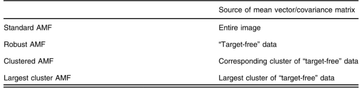
The standard AMF and three variants of the AMF are implemented in this research. The first method is the standard AMF as described above, where the mean vector and covariance matrix are taken from the entire image. The first variant, called robust AMF, is suggested by the quote from Manolakis et al.3in the Introduction. In this method, an anomaly detector analyzes the image and then the mean vector and covariance matrix are estimated from the image without the detected anomalies. The second variant is referred to as clustered AMF. In this method, anomalies are removed as in robust AMF, and then the image is clustered without the detected anomalies. Each of the clusters yields a mean vector and covariance matrix estimate. Since a target pixel may be surrounded by pixels of various types (e.g., grass, trees, etc.), the cluster most represented in the collection will be referred to as the modal class The corresponding background statistics for the pixels to be classified are determined through the modal class of its neighbors. A similar idea has been proposed in anomaly detection.8 Due to the time-consuming nature of determining which cluster a pixel is located in, a third variant, called largest cluster AMF, is developed. This method removes the anomalies and clusters the resulting data as is done in clustered AMF. However, the mean vector and covariance matrix for the pixels to be classified are estimated from the single largest cluster of data in the image. Table1is provided to show the source of mean vectors and covariance matrices for the implemented AMFs.
2.3
Atmospheric Compensation
Spectral signature matching within HSI typically incorporates a spectral library consisting of ground-measured reflectance data from objects of interest. The difficulty with spectral signature matching is that hyperspectral images are collected using a sensor that collects pupil-plane radi-ance, which includes reflected and radiated energy as well as atmospheric distortions. Before spectral signatures from an image can be compared to target signatures, atmospheric compen-sation must be performed to bring the spectral library from the reflectance space to the pupil-plane radiance space. Since radiance data is a function of atmospheric conditions, which vary greatly by collection time, the spectral library must be processed with each image separately.9 Linear and model-based approaches are available to transform data from the reflectance space to the radiance space. Model-based approaches, such as MODTRAN,10 require prior knowledge about the scene collection. Precise computation of radiance from reflectance values is elusive. A linear method called the empirical line method (ELM) was chosen for its simplicity and its ability to work well in controlled scenes such as the ones used here.9 Although more computationally intensive atmospheric compensation methods are available, ELM, the normal-ized difference vegetation index (NDVI), and the bare soil index (BI) offer a way to compute a linear, and intuitively understandable, transformation between reflectance to radiance without complicated formulas, models, or nonlinear methods. Additionally, ELM is a reputable and well-known method; it is noted as offering simplicity and quality in controlled environ-ments.4,9,11–14This research is not focused on developing or testing new atmospheric compen-sation methods; rather, it is focused on developing a new classification method.
Table 1 Source of mean vectors and covariance matrices for the implemented AMFs.
Source of mean vector/covariance matrix Standard AMF Entire image
Robust AMF “Target-free”data
Clustered AMF Corresponding cluster of“target-free”data Largest cluster AMF Largest cluster of“target-free”data
Linear methods assume that atmospheric content is a linear addition where the pupil-plane radiance is a function of reflectance with a scaling multiplier and offset:
Li¼aρiþb; (3)
whereρiis a reflectance signature to be transformed into theLiradiance space with gain,a, and offset,b, as calculated by a¼L2−L1 ρ2−ρ1 (4) b¼L1ρ2−L2ρ1 ρ2−ρ1 ; (5)
whereρ1andρ2are known reflectance signatures from the spectral library, andL1andL2are the corresponding radiance measurements from the scene. Linear methods are comprised of two general types: methods such as ELM, which require known objects of interest to be within the spectral library and located within the image; and vegetation normalization methods, which use expected radiance and reflectance of vegetation in place of specific known objects. Both permit atmospheric compensation to be conducted for the remaining objects in the spectral library.9
For situations lacking prior knowledge of scene content, methods such as vegetation nor-malization are appropriate, where the linear method in Eq. (3) is applied with radiance measure-ments for materials expected in the scene. The NDVI and the BI are two methods that allow atmospheric compensation to be performed depending on the scene landcover.9
2.3.1
Normalized difference vegetation index
NDVI15is a method that is used to determine whether a pixel within a hyperspectral image is
green vegetation. It does this by comparing the radiance of the near infrared (NIR) spectrum to the red spectrum
NDVI¼NIR−red
NIRþred; (6)
where red corresponds to the 600 to 700-nm bands and NIR corresponds to the 700 to 1000-nm near-infrared bands.9 In this research, we used bands corresponding to 660 nm for red and
860 nm for NIR.
NDVI is calculated for each pixel within an image, and pixels with the highest scores can be used as vegetation within the radiance space. Hence, the vegetation in the spectral library can be used asρ2in Eqs. (4) and (5), and the average spectral signature of the pixels with the highest NDVI score can be used asL2.L1can be determined from the shadows within an image which can be estimated by the spectral signature, which is calculated by taking the minimum value from each band in the image across all pixels. Finally,ρ1is set as a vector of zeros, and interpreted as the ideal minimum radiance in the image.9
2.3.2
Bare soil index
BI16is a method similar to NDVI; however, it is designed for bare soil within a hyperspectral
image. It can be employed in the same fashion as NDVI, assuming that there is a soil meas-urement within the spectral library:
BI¼ððSWIRþredÞ−ðNIRþblueÞ
SWIRþredÞ þ ðNIRþblueÞ; (7) where blue corresponds to the 450 to 500-nm bands, red corresponds to the 600 to 700-nm bands, NIR corresponds to the 700 to 1000-nm bands, and short wave infrared (SWIR)
corresponds to the 1150 to 2500-nm SWIR bands.9In this research, we used the band corre-sponding to 470 nm for blue, 660 nm for red, 860 nm for NIR, and 2280 nm for SWIR.
3 Anomaly Detection Algorithms
To apply an anomaly detection algorithm to hyperspectral data, first the atmospheric absorption bands should be removed and the data cube must be reshaped into a data matrix. The removal of the absorptions bands in the images employed in this research results in the retention of 145 of the 210 original bands. HSI data is typically stored in a three-dimensional matrix, referred to as an image cube or a data cube, with the first two dimensions of the matrix being the location of the pixel in the image and the third dimension being the magnitude at each of the recorded electro-magnetic bands. Therefore, it can be viewed as a stack of images, with each image representing the intensity of a given band. Ann×pdata matrix is generated by reshaping the data cube into a matrix with the first dimension containing allnpixels in the image and the second dimension containing allpbands. After the data is in the proper form, principal component analysis (PCA17 is employed as a data reduction tool. In all the algorithms except autonomous global anomaly detector (AutoGAD), the user is left to determine the number of principal components (PCs) to retain in order to reduce the dimensionality of the data.
3.1
RX Detector
The RX algorithm, developed by Reed and Yu,18detects anomalies through the use of a moving window. The pixel in the center of the window is scored against the other pixels in the window. The window is then shifted by one pixel and the process is repeated until each pixel,x, has received anRXðxÞscore based on
RXðxÞ ¼ ðx−μÞT N Nþ1 X þ 1 Nþ1 ðx−μÞðx−μÞT −1 ðx−μÞ; (8)
whereNis the number of pixels in the window andμandPare the estimated mean and covari-ance matrix of the data within the window. Pixels are considered anomalous if their RX score is greater than a chi-squared distribution with corresponding significance level, α, and N−1 degrees of freedom.
3.2
Iterative RX Detector
The iterative RX (IRX) detector was introduced by Taitano et al.19as an extension to the RX detector in an attempt to mitigate the effects that anomalies have on mean vector and covariance matrix calculations. The algorithm runs RX in an iterative fashion, each time removing pixels flagged in the previous iteration as anomalous from the mean vector and covariance statistics used to calculate the RX scores. This process continues until the set of anomalies in the previous iteration matches the set from the current iteration or the maximum number of iterations has been completed.19
3.3
Linear RX and Iterative Linear RX Detectors
The linear RX (LRX) and iterative linear RX (ILRX) detectors20function in the same manner as the RX and IRX except that a vertical line of data is used as opposed to a window. If the number of pixels selected for the line size is larger than the image, then pixels are taken from the bottom of the previous column and the top of the subsequent column. These methods are better than the previously described methods because they increase the average distance between the test pixel and the pixels used to estimate the background statistics, thereby decreasing the effects of cor-relation due to spatial proximity.20
3.4
Autonomous Global Anomaly Detector
The AutoGAD21is an independent component analysis (ICA)22,23based detector that is proc-essed in four phases. Phase I reduces the dimensionality of the data through PCA17, using the
geometry of the eigenvalue curve to determine the number of PCs to retain. Phase II conducts ICA on the retained PCs from Phase I via the FastICA algorithm.24 Phase III determines the independent components (ICs) that potentially contain anomalies using two filters: the potential anomaly signal-to-noise ratio and the maximum pixel score. Phase IV smooths the background noise in the ICs selected in Phase III using an adaptive Wiener filter25in an iterative fashion, and then locates the potential anomalies using the zero bin method described by Chiang et al.26
3.5
Support Vector Data Description
Support vector data description (SVDD) was originally applied to HSI data by Banerjee et al.27,28 SVDD is a semi-supervised algorithm that requires a training set of background data. Since HSI images are usually assumed to contain few anomalies, the training set is generated by randomly selecting pixels from the image. The minimum volume hypersphere about the training set,
S¼ fx∶kx−ak2 <R2g, is then calculated with centeraand radiusR. The hypersphere is
deter-mined through constrained Lagrangian optimization that simplifies to SVDDðyÞ ¼R2−Kðy; yÞ þ2X
i
αiKðy; xiÞ; (9)
whereKðx; yÞis the kernel mapping defined by
Kðx; yÞ ¼expð−kx−yk2∕σ2Þ; (10)
andyis the pixel of interest, andαi are the weights or support vectors, andσ2 is a radial basis
function parameter used to scale the size of the hypersphere. Finally, pixels that have a SVDD score larger than a user-defined threshold are considered anomalies.27,28
3.6
Blocked Adaptive Computationally Efficient Outlier Nominators
Blocked adaptive computationally efficient outlier nominators (BACON) is a statistical outlier detector created by Billor et al.29It attempts to locate outliers in a data set through the use of iterative estimates of the model with a robust starting point. The algorithm is computationally efficient, regularly requiring fewer than five iterations to converge, so it is applicable to HSI data. The basic idea is to start with a small subset of outlier-free data and iteratively add blocks of data to the data set until all data points not considered outliers are in the data set. The final data set is then assumed to be outlier free and thus can be used to generate robust mean vector and covari-ance matrix estimates.29
The BACON algorithm begins by selecting an initial basic subset of data withm¼cpdata points with the smallest Mahalanobis distance, where in the case of HSIpis equal to the number of bands within image andc¼4or 5, as suggested by Billor et al.,29so long asm≥nwherenis
the number of pixels in the image. Next, the Mahalanobis distances are calculated for each of the pixels, remembering thatμand Σare now the mean vector and covariance matrix of the basic subset. A new basic subset of all of the pixels with distances less than cnprχ2
p;α∕2 is selected,
where χ2
p;α∕n is the 1−ðα∕nÞsignificance level of a chi-squared distribution with p degrees of freedom andcnpr¼cnpþchr is the correction factor, where
cnp¼1þpþ1 n−pþ 2 n−1−3p; (11) chr¼max 0;ððhhþ−rrÞÞ ; (12)
h¼ðnþpþ1Þ
2 : (13)
Here,ris the size of the current basic subset,nis the number of observations, or pixels, andp is the dimensionality of the data, or bands. If the size of the new basic subset is the same size of the basic subset from the previous iteration, the algorithm is terminated. Otherwise, a new basic subset is calculated.29
4 Clustering
Cluster analysis is a multivariate analysis technique for grouping, or clustering, a dataset into smaller subsets known asclusters.The goal of cluster analysis is to maximize the between-cluster variation while minimizing intra-cluster variation.30K-means is a clustering technique where the data is split intokuser-defined number of clusters. TheK-means algorithm is initialized by ran-domly selectingkstarting points, or cluster centers. Next, a random data point is selected and added to the nearest cluster. The corresponding cluster center is then updated with the new data, allowing for currently clustered data to move into other clusters. This process is repeated until all the data points are in one of thekclusters and no data points are moved in an iteration of the algorithm.30 The difficulty when using a clustering algorithm such asK-means is selectingk, the number of clusters.X-means is a clustering algorithm based uponK-means and has the advantage of being able to select the number of clusters from a user-defined range as opposed to a single value. This is accomplished by runningK-means multiple times, splitting each of the original clusters in two, and scoring each possible subset of full and partial clusters using the Bayesian infor-mation criterion (BIC) to determine the optimal clustering.31
Rather than supplying the X-means algorithm the specific number of clusters as in
K-means, the user defines a range of possible clusters,k-lower and k-upper. In this research, theX-means algorithm was implemented withk-lower andk-upper set to 3 and 10, respectively. The algorithm begins by runningK-means on the data set withkequal tok-lower. Next, each of the originalkclusters are split in two usingK-means, withkequal to 2. Then all2k possible combinations of whole clusters and split clusters are analyzed for the corresponding BIC scores. Thenkis incremented and the process is repeated untilk-upper has been analyzed. The algorithm then returns thekcluster centers with the highest corresponding BIC score, andK-means is run one last time using the returned cluster centers as the initial starting points.31
5 Methodology
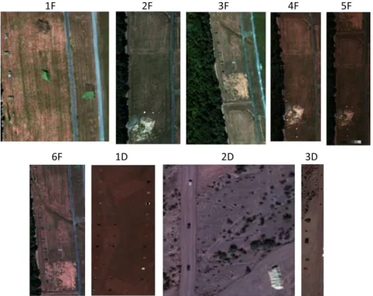
The images used in this research come from the hyperspectral digital imagery collection equip-ment32sensor for the Forest Radiance I and Desert Radiance II collection events in 1995. The images were collected with 210 bands between 397 and 2500 nm and the ground reflectance data was collected with 430 bands between 350 and 2500 nm. The collection names allude to images consisting of forest and desert scenes. Nine images were employed in this research: six forest images and three desert images (as shown in Fig.1and with image details displayed in Table2). Atmospheric compensation was performed with NDVI for forest images, and BI was applied for the desert images due to the lack of vegetation. The targets (which constitute the anomalies of interest herein) in the images consists of vehicles, various colored fabrics and tarps, and numer-ous types of metals and other building materials.
The first step was to analyze an image using one of the seven anomaly detectors described in Sec.3: RX, IRX, LRX, ILRX, AutoGAD, SVDD, or BACON. Each algorithm has user-defined settings that influence the algorithms’performance. In these experiments, the RX detectors and SVDD used the best settings as reflected in Williams et al.,20the settings for AutoGAD were taken from Johnson et al.,21 and the settings for BACON were taken from Billor et al.29 The anomalies detected by the anomaly detector were used twice: first, the anomalies were removed from the image to calculate a robust mean vector and covariance matrix, and second, the anoma-lous pixels served as the test pixels to be classified using one of the four AMF variants described in Sec.2.2: standard AMF, robust AMF, clustered AMF, and largest cluster AMF.
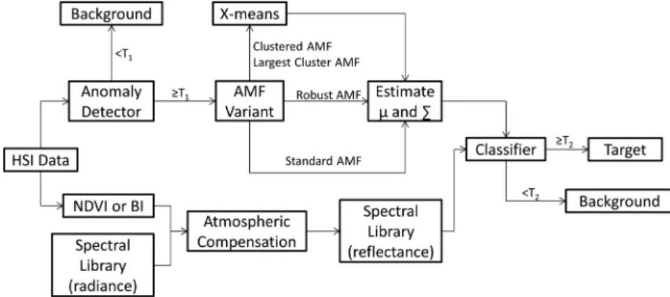
The following steps were performed to classify anomalies. First, the spectral library, con-sisting of 30 objects for forest images and 34 objects for desert images, was transformed from reflectance space to radiance space using NDVI or BI atmospheric compensation depend-ing on the image scene, as depicted in the bottom of Fig.2. Next, one of the seven anomaly detectors then analyzed the image for anomalous pixels, as shown in the top of Fig.2. Pixels below the anomaly detector threshold (T1) are classified as background. Pixels above T1 are classified as anomalies and are used as the pixels to be classified by the AMFs. The mean vector (μ) and covariance matrix (P) are estimated using the appropriate set of data for the AMF vari-ant. The standard AMF usesμandPfrom the entire image, the robust AMF usesμandPfrom
Fig. 1 Hyperspectral images.
Table 2 Hyperspectral image data.
Image Size Total pixels Anomalous pixels Anomalies Unique targets 1F 191×160 30,560 994 10 5 2F 312×152 47,424 281 30 9 3F 226×136 30,736 96 20 11 4F 205×80 16,400 75 29 12 5F 470×156 73,320 440 15 20 6F 355×150 53,250 976 45 10 1D 215×104 22,360 490 46 22 2D 156×156 24,336 417 4 3 3D 460×78 35,880 405 12 12
the image without the detected anomalies, and the clustered AMF and largest cluster AMF use μ and P from the appropriate cluster of data, as determined by the X-means algorithm. Finally, the data is processed through the classifier, and pixels below the classifier threshold (T2) are classified as background and pixels aboveT2 are classified as appropriate target types.
In order to generate receiver operating characteristic (ROC)—like curves33for each AMF/ anomaly detector pair across all nine test images, the following methodology was employed. Each anomaly detector was run across a range of anomaly detector thresholds (Ti1), i¼1;2; : : : ;19 where T1
1 ¼0.01, Ti1þ1¼Ti1þΔ1, and Δ1¼0.005. The pixels flagged as
anomalous are then processed through the four AMFs. Each target in the spectral library is com-pared to a pixel of interest, and the target type with the largest resulting AMF score is declared given its score is above the AMF threshold (Tj2), j¼1;2; : : : ;100 where T1
2¼0.01,
Tjþ1 2 ¼T
j
2þΔ2, and Δ2¼0.01. The thresholding implemented in this research is created
by finding the range of all the AMF scores corresponding to the target type with the largest resulting AMF score and normalizing them between 0 and 1 to allow for consistency among the different AMFs within an image. When a threshold is selected, any pixel with an AMF score less than the threshold is classified as background. Analyzing each of the different detector thresholds across all four of the AMFs, while allowingTj2 to vary across its range of possible values, enumerates all combinations ofTi1 and Tj2.
As the images are processed, a2×3confusion matrix, as displayed in Table3, was generated for eachTi1,Tj2, image combination, denotedCTi
1T
j
2ðkÞ
, whereiandjrepresent specific threshold values andkis the image of interest. The confusion matrix is comprised of two sections to allow for the scoring of every pixel in the image. The anomaly detector section reflects the declaration of a test pixel as background or the passing of the pixel to be classified. Relative to the detector declaration of background, there are false negatives (FNs) and true negatives (TNs). The anomaly classifier section then reflects the ultimate classification of the pixels classified as anomalous by the anomaly detector.
After each of the nine images are processed, new2×3confusion matrices are generated that consist of the sum across all nine images for eachCk
Ti
1T
j
2
combination defined by Fig. 2 Classification experimental process graph.
Table 3 2×3Confusion matrix.
Anomaly detector Anomaly classifier
Background Target Background Target False negative (detector) True positive (classifier) False negative (classifier) Background True negative (detector) False positive (classifier) True negative (classifier)
CTi 1T j 2 ¼ XI k¼1 CTi 1T j 2ðkÞ; (14)
whereIis the number of images analyzed, hereI¼9. Below, the true positive fraction (TPF) (classifier) versus false positive fraction (FPF) (classifier) data point for eachCTi
1Tj2was plotted
for a given anomaly detector—anomaly classifier combination, and the convex hull of the result-ing data is interpreted as a rough ROC curve, as is shown notionally in Fig.3, where the circles are data points and the line represents the ROC curve.
6 Results
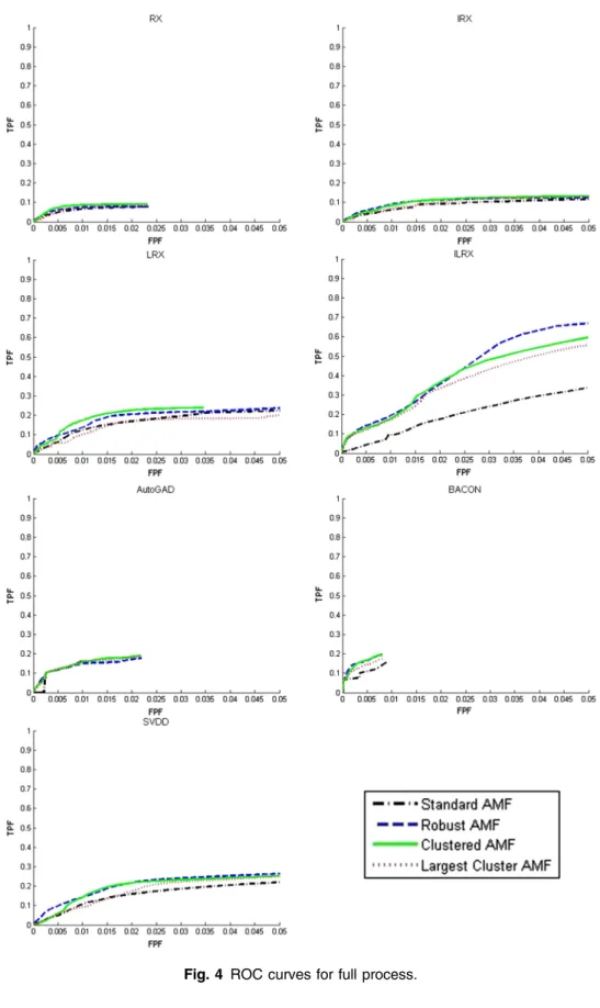
The four AMFs and the seven anomaly detectors were scored to produce ROC curves as described in Sec.5, with the results shown in Figs.4and5. Each figure contains separate graphs of classification performance generated from each anomaly detector. Figure4shows the ROC curves for the full process (detection plus classification). This means taking into account the full 2×3 confusion matrix, implying that
TPF¼ TPC TPCþFNCþFND (15) FPF¼ FPC FPCþTNCþTND ; (16)
where the subscript C and D denote classifier and detector, respectively. Note the low TPF and extremely small FPF come from the fact that nine images with a total of 334,226 pixels were analyzed in the process and these statistics are biased downward by a large number of FND andTND. The key insight to be gained from these ROC curves is that in all cases, the
variants outperform the standard AMF. Furthermore, the clustering methods enhance the robust AMF.
To get a better visualization of the data, a set of conditional ROC curves were created. Figure5displays the ROC curves which account for the performance of the AMF given detec-tions, implying that
TPF¼ TPC TPCþFNC
(17) Fig. 3 ROC curve generated from convex hull of data.
FPF¼ FPC FPCþTNC
: (18)
Again, we see the variants outperform the standard AMF, and in most cases, the clustering methods enhance the robust AMF.
7 Conclusions
This article demonstrates improvements to AMF performance by addressing correlation and nonhomogeneity problems inherent to HSI data, which are often ignored when classifying anomalies. The standard AMF and three variants were employed along with seven different anomaly detectors utilized prior to classification. Manolakis et al.3 state the estimation of
the mean vector and covariance matrix should be calculated using“target-free”data, generating a robust AMF. Here, it was shown that accounting for spatial correlation effects in the detector yields nearly“target-free”data for use in an AMF that is greatly improved through the use of cluster analysis methods.
References
1. G. Shaw and D. Manolakis,“Signal processing for hyperspectral image exploitation,”IEEE Signal Process. Mag.19(1), 12–16 (2002),http://dx.doi.org/10.1109/79.974715.
2. D. A. Landgrebe,“Hyperspectral image data analysis,”IEEE Signal Process. Mag.19(1), 17–28 (2002),http://dx.doi.org/10.1109/79.974718.
3. D. Manolakis et al.,“Is there a best hyperspectral detection algorithm?,”Proc. SPIE7334, 1–16 (2009),http://dx.doi.org/10.1117/12.816917.
4. M. T. Eismann, A. D. Stocker, and N. M. Nasrabadi,“Automated hyperspectral cueing for civilian search and rescue,” Proc. IEEE 97(6), 1031–1055 (2009), http://dx.doi.org/10 .1109/JPROC.2009.2013561.
5. T. E. Smetek and K. W. Bauer,“A comparison of multivariate outlier detection methods for finding hyperspectral anomalies,”Mil. Oper. Res.13(4), 19–44 (2008),http://dx.doi.org/10 .5711/morj.13.4.19.
6. D. Manolakis et al.,“Maintaining CFAR operation in hyperspectral target detection using extreme value distributions,”Proc. SPIE6565, 1–32 (2007), http://dx.doi.org/10.1117/12 .718373.
7. D. Manolakis and G. Shaw, “Detection algorithms for hyperspectral imaging applications,” IEEE Signal Process. Mag. 19(1), 29–43 (2002), http://dx.doi.org/10 .1109/79.974724.
8. D. Stein, A. Stocker, and S. Beaven,“The fusion of quadratic detection statistics applied to hyperspectral imagery,”inIRIA-IRIS Proc. 2000 Meeting of the MSS Specialty Group on Camouflage, Concealment, and Deception, pp. 271–280 (2000).
9. M. T. Eismann, Hyperspectral Remote Sensing, SPIE Press, Bellingham, WA (2012). 10. A. Berk et al., “MODTRAN4: radiative transfer modeling for atmospheric correction,”
Proc. SPIE3756, 348–353 (1999),http://dx.doi.org/10.1117/12.366388.
11. E. Karpouzli and T. Malthus,“The empirical line method for the atmospheric correction of IKONOS imagery,”Int. J. Rem. Sens.24(5), 1143–1150 (2003),http://dx.doi.org/10.1080/ 0143116021000026779.
12. G. M. Smith and E. J. Milton,“The use of the empirical line method to calibrate remotely sensed data to reflectance,”Int. J. Rem. Sens.20(13), 2653–2662 (1999),http://dx.doi.org/ 10.1080/014311699211994.
13. N. A. S. Hamm, P. M. Atkinson, and E. J. Milton,“A per-pixel, non-stationary model for empirical line atmospheric correction in remote sensing,”Rem. Sens. Environ.124, 666– 678 (2012),http://dx.doi.org/10.1016/j.rse.2012.05.033.
14. W. M. Baugh and D. P. Groeneveld,“Empirical proof of the empirical line,”Int. J. Rem. Sens.29(3), 665–672 (2008),http://dx.doi.org/10.1080/01431160701352162.
15. J.W. Rouse et al.,“Monitoring vegetation systems in the Great Plains with third ERTS,”in
Proc. ERTS Symp., NASA no. SP-351, pp. 309–317, NASA, Goddard Space Flight Center, Washington, DC (1973).
16. W. Chen et al.,“Monitoring the seasonal bare soil areas in Beijing using multi-temporal TM images,”inProc. IEEE Int. Geosci. Rem. Sens. Symp., Anchorage, AK, Vol. 5, pp. 3379– 3382 (2004).
17. D. A. Landgrebe,Signal Theory Methods in Multispectral Remote Sensing, John Wiley & Sons, Hoboken, NJ (2003).
18. I. S. Reed and X. Yu,“Adaptive multiple-band CFAR detection of an optical pattern with unknown spectral distribution,”IEEE Trans. Acoust. Speech Signal Process.38(10), 1760– 1770 (1990),http://dx.doi.org/10.1109/29.60107.
19. Y. P. Taitano, B. A. Geier, and K. W. Bauer,“A locally adaptable iterative RX detector,”
EURASIP J. Adv. Signal Process. Special Issue on Adv. Image Proc. Defense Secur. Appl.
20. J. P. Williams, T. J. Bihl, and K. W. Bauer,“Towards the mitigation of correlation effects in anomaly detection for hyperspectral imagery,”J. Defense Model. Simul.(in press). 21. R. J. Johnson, J. P. Williams, and K. W. Bauer,“AutoGAD: an improved ICA based
hyper-spectral anomaly detection algorithm,”IEEE Trans. Geosci. Rem. Sens.51(6), 3492–3503 (2013),http://dx.doi.org/10.1109/TGRS.2012.2222418.
22. A. Hyvärinen, J. Karhunen, and E. Oja, Independent Component Analysis, Wiley-Interscience, New York (2001).
23. J. V. Stone, Independent Component Analysis: A Tutorial Introduction, MIT Press, Cambridge, MA (2004).
24. A. Hyvärinen,“Fast and robust fixed-point algorithms for independent component analysis,”
IEEE Trans. Neural Netw.10(3), 626–634 (1999),http://dx.doi.org/10.1109/72.761722. 25. J. S. Lim,Two-Dimensional Signal and Image Processing, Prentice Hall PTR, Englewood
Cliffs, NJ (1990).
26. S-S. Chiang, C.-I. Chang, and I. Ginsberg,“Unsupervised target detection in hyperspectral images using projection pursuit,” IEEE Trans. Geosci. Rem. Sens. 39(7), 1380–1391 (2001),http://dx.doi.org/10.1109/36.934071.
27. A. Banerjee, P. Burlina, and C. Diehl,“A support vector method for anomaly detection in hyperspectral imagery,”IEEE Trans. Geosci. Rem. Sens.44(8), 2282–2291 (2006),http://dx .doi.org/10.1109/TGRS.2006.873019.
28. A. Banerjee, P. Burlina, and R. Meth,“Fast hyperspectral anomaly detection via SVDD,”in
Proc. IEEE Int. Conf. Image Proc., Vol. 4, pp. 101–104, Curran Associates, San Antonio, TX (2007).
29. N. Billor, A. S. Hadi, and P. F. Velleman, “BACON: blocked adaptive computationally efficient outlier nominators,” Comput. Stat. Data Anal. 34, 279–298 (2000), http://dx .doi.org/10.1016/S0167-9473(99)00101-2.
30. W. R. Dillon and M. Goldstein, Multivariate Analysis: Methods and Applications, John Wiley and Sons, New York (1984).
31. D. Pelleg and A. Moore,“X-means: extendingK-means with efficient estimation of the number of clusters,” in Proc. 17th Int. Conf. Mach. Learn., pp. 727–734, Morgan Kaufmann, Stanford, CA (2000).
32. L. J. Rickard et al.,“HYDICE: an airborne system for hyperspectral imaging,”Proc. SPIE
1937, 173–179 (1993), http://dx.doi.org/10.1117/12.157055.
33. T. Fawcett, “An introduction to ROC analysis,” Pattern Recogn. Lett. 27(8), 861–874 (2006),http://dx.doi.org/10.1016/j.patrec.2005.10.010.
Jason P. Williamsreceived a BS degree in mathematics from the University of Illinois, Urbana, in 2001 and MS and PhD degrees in operations research from the Air Force Institute of Technology, Wright-Patterson Air Force Base, OH, in 2007 and 2012, respectively. He is cur-rently with the Headquarters U.S. Air Forces in Europe, Ramstein Air Base, Germany. His research interests are in the areas of multivariate statistics and response surfaces.
Kenneth W. Bauerreceived a BS degree from Miami University, Oxford, OH, in 1976, an MEA degree from the University of Utah, Salt Lake City, UT, in 1980, an MS degree from the Air Force Institute of Technology, Wright-Patterson Air Force Base, OH, in 1981, and a PhD degree from Purdue University, West Lafayette, IN, in 1987. He is currently a professor of operations research with the Air Force Institute of Technology, where he teaches classes in applied statistics and pattern recognition. His research interests lie in the areas of automatic target recognition and multivariate statistics.
Mark A. Friendreceived his BS from Texas Christian University in 1996 and MS and PhD degrees in operations research from the Air Force Institute of Technology, Wright-Patterson Air Force Base, OH, in 1998 and 2007, respectively. He currently serves as a lieutenant colonel in the United States Air Force stationed at Wright-Patterson AFB, OH, where he is an assistant pro-fessor in the Department of Operational Sciences at the Air Force Institute of Technology. His research interests lie in the areas of automatic target recognition, applied statistics, and simulation.