TI 2011-023/4
Tinbergen Institute Discussion Paper
An Alternative Bayesian Approach to
Structural Breaks in Time Series
Models
Sjoerd van den Hauwe
Richard Paap
Dick J.C. van Dijk
Econometric Institute, Erasmus School of Economics, Erasmus University Rotterdam, and Tinbergen Institute.
Tinbergen Institute is the graduate school and research institute in economics of Erasmus University Rotterdam, the University of Amsterdam and VU University Amsterdam. More TI discussion papers can be downloaded at http://www.tinbergen.nl
Tinbergen Institute has two locations: Tinbergen Institute Amsterdam Gustav Mahlerplein 117 1082 MS Amsterdam The Netherlands Tel.: +31(0)20 525 1600 Tinbergen Institute Rotterdam Burg. Oudlaan 50
3062 PA Rotterdam The Netherlands Tel.: +31(0)10 408 8900 Fax: +31(0)10 408 9031
Duisenberg school of finance is a collaboration of the Dutch financial sector and universities, with the ambition to support innovative research and offer top quality academic education in core areas of finance.
DSF research papers can be downloaded at: http://www.dsf.nl/
Duisenberg school of finance Gustav Mahlerplein 117 1082 MS Amsterdam The Netherlands Tel.: +31(0)20 525 8579
An Alternative Bayesian Approach to
Structural Breaks in Time Series Models
Sjoerd van den Hauwe
1,2∗Richard Paap
1,2Dick van Dijk
1,21Econometric Institute
Erasmus University Rotterdam 2Tinbergen Institute
February 7, 2011
Abstract
We propose a new approach to deal with structural breaks in time series models. The key contribution is an alternative dynamic stochastic specification for the model parameters which describes potential breaks. After a break new parameter values are generated from a so-called baseline prior distribution. Modeling boils down to the choice of a parametric likelihood specification and a baseline prior with the proper support for the parameters. The approach accounts in a natural way for potential out-of-sample breaks where the number of breaks is stochastic. Posterior inference involves simple computations that are less demanding than existing methods. The approach is illustrated on nonlinear discrete time series models and models with re-strictions on the parameter space.
Keywords: Structural breaks, Bayesian analysis, forecasting, MCMC methods, non-linear time series.
JEL Classification: C11, C22, C51, C53, C63.
∗We thank John Geweke and other participants of the first European Seminar on Bayesian
Econometrics in 2010 in Rotterdam for helpful comments. Corresponding author: Sjoerd van den Hauwe, Tinbergen Institute, Erasmus University Rotterdam, P.O. Box 1738, NL-3000 DR Rotterdam, The Netherlands. Tel.: +31-10-40811298, Fax: +31-10-4089162. E-mail address:
1
Introduction
Over the last two decades, empirical evidence showing that macroeconomic and fi-nancial time series are subject to occasional structural breaks in their statistical properties has mounted, see Stock and Watson (1996) and Andreou and Ghysels (2009), among many others. A prominent example in macroeconomics is the Great Moderation, referring to the large decline in volatility experienced by many macroe-conomic time series in the first half of the 1980s, see McConnell and Perez-Quiros (2000); Stock and Watson (2002); Sensier and van Dijk (2004) and Kim et al. (2008), among others. In finance, the presence of structural breaks in predictive regres-sion models for asset returns is by now well documented, see Pesaran and Timmer-mann (2002); Paye and TimmerTimmer-mann (2006); Rapach and Wohar (2006); Lettau and Van Nieuwerburgh (2008); Ravazzolo et al. (2008) and Pettenuzzo and Timmermann (forthcoming), among others.
Many empirical studies reporting evidence for structural changes in macroeco-nomic and financial time series make use of frequentist methods for detecting and dating such breaks, as developed by Andrews (1993); Andrews and Ploberger (1994); Bai and Perron (1998); Bai et al. (1998) and Qu and Perron (2007), among others; see Perron (2006) for a recent survey. These methods can be classified as ‘histor-ical’ testing procedures (Andreou and Ghysels; 2009), in the sense that they are designed for testing for structural change and the identification of potential break dates ex-post for time series observations spanning a given historical, in-sample pe-riod.1 Out-of-sample forecasting in the presence of structural breaks has presented
a much bigger challenge when relying upon frequentist methods, see the survey of Clements and Hendry (2006). A Bayesian approach would much better suit this problem, in the sense that structural change can be made an inherent part of the statistical time series model, in particular including the possibility that breaks oc-cur in the out-of-sample period. Surprisingly then, accounting for possible future breaks when constructing out-of-sample forecasts has not received much attention in the Bayesian literature on structural breaks, with the notable exceptions of Pesaran et al. (2006), Koop and Potter (2007), Maheu and Gordon (2008), and Geweke and
1A different strand of literature concerns testing for structural change ‘in real time’, i.e.
mon-itoring whether new, incoming observations are consistent with a previously specified model, see Chu et al. (1996) and Zeileis et al. (2005), among others.
Jiang (2010).
In this paper we propose a new Bayesian approach to deal with structural breaks in time series models, with an explicit focus on the implications for out-of-sample forecasting. Following the previous literature, we define a structural break as a permanent change in the value of a parameter of the model or, in the Bayesian framework, of a likelihood function. We propose a new stochastic specification to describe the dynamic behavior of the parameter, which has a simple and intuitively appealing interpretation. In each period, with a particular probability a structural break occurs and in that case the new parameter value is generated by a so-called baseline prior distribution. If a break does not occur, the parameter value is equal to the value in the previous period. Put differently, the (conditional) distribution of the model parameter is a two-component mixture, where one component is the baseline prior distribution and the other component is degenerate at the parameter value in the previous period. The mixing probability for the first component is the probability of a structural break. The key advantage of this specification lies in the Bayesian procedures for estimation and forecasting. For estimation purposes, we derive a Markov chain Monte Carlo [MCMC] based algorithm for simulating from the posterior distribution of the model parameters. The posterior simulator boils down to straightforward sampling from three-component mixture distributions, where most weight is put on degenerate components. Our sampler is a single-move algorithm, for which it is well-known that convergence may be problematic (or at least slow). To solve this issue, we introduce a remix step in our sampler which bears similarities to the remixing step in Dirichlet process prior models. For forecasting purposes, the predictive distributions of future observations are also of the mixture type, with one component being the model under the no-break scenario and the other being the model integrated over the baseline prior in case of a break. If the forecast horizon grows, the probability of a break in the out-of-sample period increases and the latter mixture component gets more weight.
The baseline prior and its hyperparameters form a key component in forecasting exercises. Our model specification is such that in the case of a structural break the new parameter value is independently from the past drawn from this baseline prior distribution. However, by including a third layer in the model, this independence assumption may be relaxed and we can train the hyperparameters of the baseline
distribution. Such a strategy is common in marketing (see for example Rossi et al.; 2005) and applied to structural break models in Carlin et al. (1992), Pesaran et al. (2006) and Geweke and Jiang (2010). By doing so, regimes from the past do reveal information for future parameter values that is properly absorbed by the predictive distribution.
Our methodology to accommodate structural breaks in time series models is closely related to the independent, contemporary research by Geweke and Jiang (2010) and the methods by Maheu and Gordon (2008), who propose essentially a similar specification. However, we employ a different submodel representation for the dynamic behavior of the model parameters with favorable computational implica-tions. The simulator of Geweke and Jiang (2010) requires that the regime parameters can be marginalized analytically. But, this requirement restricts the combinations of model and baseline prior distribution that can be considered. Moreover, their sam-pler requires potentially cumbersome tuning of the Metropolis–Hastings proposal distributions. Our simulator does not have these restrictions and can in principle be applied to any combination of model and baseline prior distribution. Maheu and Gordon (2008) also restrict their analysis to models in which the posterior distri-bution is of known form and, moreover, their estimation procedures require com-putationally intensive marginal likelihood evaluations and continuously updating of posterior model probabilities over time.
Our approach to structural breaks in fact offers two key advantages compared to other existing methods. Both are closely related to the desirable properties of structural break models as formulated by Koop and Potter (2007). The first advan-tage is that our specification allows for ana priori unknown number and timing of breaks. In particular, our approach naturally allows for the possibility that breaks may occur beyond the in-sample period. It is commonly recognized that allowing for future breaks is a necessary ingredient for realistic out-of-sample forecasting. Previ-ous attempts to do so have certain limitations and drawbacks. Pesaran et al. (2006), for example, propose an out-of-sample extension of the Markovian model of Chib (1998). In this approach, structural breaks are modeled by means of a non-recurring Markov process, which requires the specification of the number of breaks that occur, both in- and out-of-sample, see also Koop and Potter (2007). Pesaran et al. (2006) circumvent this issue by applying Bayesian model averaging over distinct scenarios,
each with a specific number of breaks in the out-of-sample period. However, this pro-cedure is computationally cumbersome, and still requires a specific plausible choice of the maximum number of breaks to happen over the forecast horizon, which may be difficult to set.2 Our approach does not suffer from these problems by specifying
the number of breaks to be stochastic both in- and out-of-sample.
The second main advantage of our specification is its ability to deal with struc-tural breaks in various types of models. Previous approaches are confined to linear regression models (e.g. Maheu and Gordon; 2008; Geweke and Jiang; 2010) or mod-els that can, at least conditionally, be written in Gaussian state-space form, as in the dynamic mixture models advocated by Gerlach et al. (2000); Giordani et al. (2007) and Giordani and Kohn (2008). By contrast, our set-up can be applied straightfor-wardly to different types of models (or likelihood functions) as well, including models for limited dependent variables, models for count data, and to copula models for de-scribing the dependence between different time series. This flexibility is mostly due to the computational advantages offered by the proposed posterior simulator for our specification of structural breaks. This efficient sampling scheme is the result of analytically integrating out the break indicator variables. If the sample size is T, then each run of the simulator is of orderO(T) and only requires evaluations of one-observation likelihoods and sampling from simple mixtures. Other simulators first integrate with respect to the regime-specific parameters to improve convergence, see Geweke and Jiang (2010) or Gerlach et al. (2000) for a similar solution in a (condi-tional) Gaussian state-space specification. Hence, the feasibility of these approaches relies on the computational ease of this integration step.
The outline of the remainder of this paper is as follows. Section 2 introduces the dynamic specification of the breaking process, analyzes its implications for out-of-sample forecasting and describes issued related to the choice of an appropriate baseline prior distribution and the probability of a structural break. Section 3 deals with the methods to simulate from the posterior distribution. Section 4 demon-strates the usefulness and wide applicability of our methods both for descriptive in-sample analysis and for constructing out-of-sample forecasts that incorporate po-tential future parameter change. This is done by means of four applications involving
2In the most extreme, but also unlikely case, this number is equal to the length of the forecasting
different types of models, including a Poisson count data model, a copula model, a probit model and an autoregressive model. A conclusion and discussion are given in Section 5. The appendices elaborate on issues related to the theoretical results and posterior simulation.
2
Modeling structural breaks
In this section we develop our modeling framework to deal with structural breaks. In Section 2.1 we discuss the model specification in detail and we compare our approach to related alternatives. In Section 2.2 we focus on the implications of our model specification for out-of-sample forecasting. The role of the baseline prior distribution and the probability of structural change are discussed in Sections 2.3 and 2.4.
2.1
Model specification
Letytbe the time series variable of interest, which is observed in periodst= 1, . . . , T,
and letyk,l = (y
k, yk+1, . . . , yl)0, (1 ≤k < l ≤T). Hence, y1,T denotes the complete
set of time series observations in the in-sample period, which we will denote by y for notational convenience. Suppose the time series in periodt is characterized by a distribution with probability density function [pdf]p(yt|y1,t−1, θt), such that yt may
depend on its own past and a possibly time-varying parameter θt.3
At the outset, it is useful to remark that we consider the case of a single parameter
θt solely to facilitate the exposition. Our specification can easily be extended to
a multiple parameter setting. In that case, we may impose simultaneous breaks in all parameters or we may allow individual parameters to break independently while, of course, intermediate cases are possible as well. Similarly, although we restrict ourselves to univariate time series here, the modeling framework can easily be extended to a multivariate setting; see Section 4 for an illustration of both issues. To allow for infrequent structural breaks in the model parameter we propose a stochastic process for θt. Specifically, the distribution of the model parameter in
3Of course it may depend on explanatory variablesx
tas well, but to keep notation clear we do
periodt is specified by the conditional density
p(θt|θ1,t−1) =p(θt|θt−1) =πf0(θt;λ) + (1−π)I{θt=θt−1}, (t= 2, . . . , T), (1)
and θ1 ∼f0(·;λ), where 0 ≤π ≤ 1, f0 is the pdf of a distribution that we call the
‘baseline prior’ for θ, which is characterized by hyperparameters λ, and I{A} is an
indicator function that is equal to one if statement A is true and zero otherwise.4
Hence, the conditional distribution of θt is a mixture of two components. With
probabilityπ a structural break occurs such that the parameter value changes, with the new value being sampled according to the baseline priorf0, while with probability
1−π no break occurs and the distribution ofθt is degenerate at the value from the
previous period. Note that the conditional distributions in (1) result in a joint distribution forθ = (θ1, . . . , θT)0, which we denote by p(θ).
Geweke and Jiang (2010) independently propose a similar approach to deal with structural breaks. A subtle difference (yet crucial for the estimation procedure) is that they explicitly introduce binary dummy variablesst, (t = 2, . . . , T), indicating
the occurrence of a break (st = 1) or not (st = 0). Their model for the
time-dependent parameters can then be written as
p(θt|θ1,t−1,s2,t) =p(θt|θt−1, st) =f0(θt)I{st=1} I{θt=θt−1}
1−I{st=1}
,
where the break indicators st are assumed to be independent and Ber(π). This
auxiliary variable can be integrated out, which results in the same specification as in (1): p(θt|θt−1) = X st=0,1 p(θt|θt−1, st)p(st) =πf0(θt) + (1−π)I{θt=θt−1}.
Similarly, our suggested approach to structural breaks is related to the mixture innovation models of Giordani et al. (2007) and Giordani and Kohn (2008). The framework in these papers crucially depends on the assumption that the model can be written in Gaussian state-space form (at least conditionally) where the parameters
4In a statistical context where we use I
{θ=θ∗} as a distribution for θ, this means that θ is
degenerate inθ∗, that is, Pr[θ=θ∗] = 1. Our notation has the same meaning as the Dirac delta δθ∗(θ).
are treated as the states. The state equations are specified such that the parameter values are sampled from a mixture of a degenerate and a Gaussian component. Specifically, the state equation is given by
θt=θt−1+Ktηt, ηt i.i.d.
∼ N(0, ση2), (2)
where the break indicators Kt have the same statistical properties as the st above.
The state equation (2) can be written in terms of conditional density functions,
p(θt|θt−1, Kt) =Ktfη(θt−θt−1) + (1−Kt)I{θt=θt−1},
wherefη is the pdf ofηt. If we again analytically integrate out the indicator variable
we can straightforwardly see the relation to our approach:
p(θt|θt−1) =
X
Kt=0,1
p(θt|θt−1, Kt)p(Kt)
=πfη(θt−θt−1) + (1−π)I{θt=θt−1}. (3)
In case of a break (3) implies that the change in the parameter value comes from
fη. In our approachθ will be a new value from the baseline priorf0.
For computational reasons, the conditional Gaussian state-space approach re-quires fη to be the pdf of a (mixed) normal distribution, otherwise the relevant
sampling methods developed by Giordani and Kohn (2008) cannot be applied. The-oretically this would not be too restrictive as long as the support for the parameter is (−∞,∞). If, however, the support is a subset of the real line or prior beliefs restrict the region (e.g. by truncation), this approach cannot be used anymore. Our framework is much more flexible with respect to distributional assumptions of the parameters, as we can simply opt for a baseline prior f0 that has the appropriate
features. We can even impose that θ can only take discrete values. Apart from this pro, our approach has additional computational advantages, which result from working with the ‘reduced’ form where the break indicators are marginalized, as will be explained in more detail in Section 3.
Furthermore, the approach of Giordani and Kohn (2008) not only requires the (mixed) Gaussian assumption of the state equation but also of the observation equa-tion. A second major advantage of our approach is that it can be applied to any kind of parametric likelihood function p(yt|y1,t−1, θt). Hence, the time series yt may be
continuous, discrete, or even a combination of both. Moreover, any choice of baseline prior distribution for the parameters and likelihood function can be analyzed, as we will demonstrate in the discussion of the estimation procedure in Section 3 and the illustrations in Section 4.
In order to get a better understanding of the behavior implied by our chosen model specification, it is insightful to examine p(θ) by means of simulation. This is a form of prior predictive analysis as advocated by Lancaster (2004) and Geweke (2005). For initialization we should pick a baseline prior distribution with density
f0 and a breaking probability π. Two routes can be followed. In the first one we
simulate a path {θt}Tt=1 by starting with θ1 ∼ f0 and subsequently using the
con-ditional distributions p(θt|θt−1), (t = 2, . . . , T) as in (1). Alternatively, we may
initialize a pathθ and then simulate iteratively from the full conditionalsp θt|θ[−t]
for t = 1, . . . , T, where θ[−t] = (θ1, . . . , θt−1, θt+1, . . . , θT)0. The first procedure is
based on the decomposition p(θ) = p(θ1)QtT=2p(θt|θt−1), while the second one
ap-plies the Gibbs sampling principle. Because the latter also provides the basis for the posterior simulation scheme as described in Section 3, we discuss this approach in more detail.5
The model in (1) for the stochastic behavior of the parameters shows that{θt}Tt=1
is a first-order Markov chain, implying that the full conditional distribution ofθtonly
depends on its two immediate neighbors. For θt, (t = 2, . . . , T−1), collecting terms
fromp(θ) gives p θt|θ[−t] ∝p(θt|θt−1)p(θt+1|θt) ∝π2f0(θt)f0(θt+1) +π(1−π)f0(θt)I{θt+1=θt} +π(1−π)f0(θt+1)I{θt=θt−1} + (1−π)2I{θt−1=θt=θt+1}. (4)
5Note that by comparing the two simulation strategies we can also check the validity of the
Gibbs sampler. That is, we can check that it traverses the entire support of p(θ) and thereby also retrieves the marginal distributions for theθt’s, which are given by the baseline priorf0 (see
Two scenarios are possible:
Scenario 1: θt−1 =θt+1 ≡θ∗. In this case θt comes from a mixture with two
com-ponents:
θt=θ∗ with probability ∝(1−π)2+ 2π(1−π)f0(θ∗),
θt∼f0 with probability ∝π2f0(θ∗).
The first component in this mixture corresponds with the situation that the value ofθtis equal to both its neighbors’ valueθ∗, which is the case if no breaks
occur at t and t+ 1, or a single break occurs at either t or t+ 1 but the new parameter value after the break is identical to the value before. The second component captures the possibility that breaks occur at both t and t+ 1, in which case the value of θt is obtained from the baseline prior distribution f0
(and by construction the value after the break at t+ 1 is again equal to the value att−1).
Scenario 2: θt−1 6=θt+1. In this case θt comes from a mixture with three
compo-nents:
θt=θt+1 with probability ∝π(1−π),
θt=θt−1 with probability ∝π(1−π),
θt∼f0 with probability ∝π2.
In this case, the three components correspond with the possibilities that (i) no break occurs at time t and (necessarily) a break occurs at t+ 1, (ii) a break occurs at timet and no break occurs at t+ 1, (iii) breaks occur at both t and
t+ 1.
If we compare these situations, it shows that when both neighbors are the same, the probability of no break gets an intuitively expected extra ‘interaction’ weight via the last term in (4). Asθ1 andθT only have one neighbor their full conditionals indicate
that with probabilityπthey come from the baseline prior and with probability 1−π
they equal their respective neighbors, that is, θ2 and θT−1.
In sum, the full conditional distributions of the parameters are a mixture of the baseline prior f0 and one or two – depending on the scenario – degenerate
distributions. Simulating from these distributions is therefore straightforward and fast, also because the degenerate components get most weight.
2.2
Forecasting implications
One of the main reasons why times series models may perform poorly in terms of (out-of-sample) forecasting is the often incorrect assumption that model parameters are stable over time. As shown by Clements and Hendry (2001, 2006), among others, neglecting structural breaks that occur during the in-sample period may yield bi-ased forecasts. As discussed in the introduction, various (frequentist and Bayesian) methods are available for detecting and modeling in-sample breaks, which may be used to annihilate the bias. However, if breaks have occurred in the past, it is likely that further structural breaks may occur during the out-of-sample period as well. Not accounting for this possibility will result in density forecasts that are tighter – as preferred by practioners –, though an essential type of uncertainty is simply ne-glected. In this section we demonstrate the implications of our modeling framework for out-of-sample forecasting, by examining how this uncertainty with regard to the possibility of future structural breaks affects the resulting density forecasts.
In a Bayesian context, density forecasts are given by the posterior predictive dis-tribution, which combines the model structure, prior considerations and information revealed by the data. At timeτ, the posterior predictive densityp(yτ+1|y1,τ) of yτ+1
can be demarginalized as p(yτ+1|y1,τ) = Z p(yτ+1|θ1,τ+1,y1,τ)p(θ1,τ+1|y1,τ)dθ1,τ+1 = Z p(yτ+1|θτ+1,y1,τ)p(θτ+1|θτ)p(θ1,τ|y1,τ)dθ1,τ+1, (5)
by using the first-order Markov property of {θt} and the conditional independence
assumptions.6 The first two densities of the integrand in (5) are given by the
(hi-erarchical) model, while the third component is the posterior density of the model parameters based on the data up to and including time τ. If we apply the dynamic specification of the model parameters (1), this expression further breaks down to
p(yτ+1|y1,τ) =π Z p(yτ+1|θτ+1,y1,τ)f0(θτ+1)p(θ1,τ|y1,τ)dθ1,τ+1 + (1−π) Z p(yτ+1|θτ+1,y1,τ)I{θτ+1=θτ}p(θ 1,τ|y1,τ)dθ1,τ+1 =πp0(yτ+1|y1,τ) + (1−π) Z p(yτ+1|θτ,y1,τ)p(θ1,τ|y1,τ)dθ1,τ, (6) 6Conditional onθ
wherep0(yt|y1,t−1) is defined to be the marginal likelihood ofyt(possibly conditional
on the pasty1,t−1) under priorf0. This result shows that the predictive distribution
is a mixture of two components: (i) with probability π a structural break occurs, and we integrate over the baseline prior f0 that generates the new but unknown
parameter value, and (ii) with probability 1−π no break occurs, and we account for the uncertainty inθτ by integrating over the posterior distribution.
In the nested situation in which we do not allow for a structural break at τ + 1 (π = 0) the predictive distribution reduces to the second part of the sum in (6). If there is a positive probability that a break occurs in the next period, the predictive probability mass is shifted in the direction of the marginal likelihood p0(yτ|y1,τ),
resulting in a more dispersed density forecast. This mechanism becomes even more clear if we investigate longer forecast horizons, as shown next.
The predictive distribution for h periods ahead is given by7
p(yτ+h|y1,τ) =
Z
p(yτ+h|θτ+h)p(θτ+1,τ+h|θτ)p(θ1,τ|y1,τ)dθ1,τ+h.
The intermediate parametersθτ,τ+h−1can be integrated out analytically by applying Proposition A.2 in Appendix A with the marginal posterior of θτ until time τ as
initial distribution, i.e., takeg(θτ) = R p(θ1,τ|y1,τ)dθ1,τ−1. This results in
p(θτ+h|y1,τ) = Z p(θτ+1,τ+h|θτ)g(θτ)dθτ,τ+h−1 = 1−(1−π)h f0(θτ+h) + (1−π)hg(θτ+h). Therefore, θτ+h|y1,τ D
−→ f0 if the forecast horizon h becomes large. For very
large h the parameter comes approximately from the baseline prior, which makes that yτ+h|y1,τ has the marginal likelihood under f0 as its limiting distribution:
yτ+h|y1,τ D
−→ p0. Temporal dependence can be dealt with in a straightforward
way by successively simulating intermediate yt’s yτ+1,τ+h−1
from the likelihood conditional on the most recently sampled parameter value.8
To summarize, the longer the forecast horizon the more the predictive probability mass gets spread according to the marginal likelihood, and possibly shifted away
7For notational convenience, here we suppress the (direct) temporal dependencies between the
dependent variable in this expression, i.e., we writep(yt|y1,t−1, θt) =p(yt|θt).
8In case of stationary processes for y
t, this direct temporal dependence introduces a second
convergence issue and the limiting distribution is not the ‘one-observation’ marginal likelihoodp0,
from the constant parameter setting where θτ+h =θτ. This process is illustrated in
the following simple example.
Example (Forecasting issues): Consider a simple normal linear regression model 9
that allows for structural breaks in the intercept and the variance:
yt|µt, σt2 i.i.d.
∼ N(µt, σ2t), (7)
f0(µ, σ2) = fN(µ;b, σ2B)fIG2(σ2;ν, S), (8)
where we assume that any breaks in the intercept and variance occur simultane-ously. The baseline prior consists of a normal-inverted Gamma–2 distribution with hyperparametersb, B, ν andS. We examine the posterior predictive distributions for different horizons. We start forecasting at timeτ where we assume we know µτ = 5
and σ2
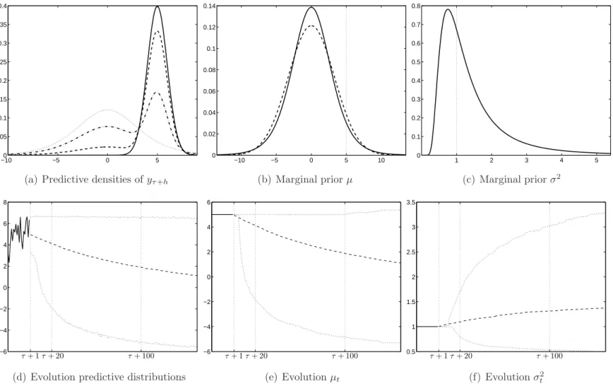
τ = 1. Figure 1 displays the forecasting characteristics in this model. The
graphs in Figure 1(a) show the predictive densities for the different horizons. The solid line shows the likelihood under µτ and στ2, which is the pdf of a normal. The
one-period ahead predictive distribution is depicted by the dashed line: we can already see the shift of probability mass due to the potential break. The dashed-dotted line is associated with h = 20. Obviously, the larger horizon h the closer the marginal likelihood (dotted line) is approximated; for h = 100 we are near the dotted line. Note that in this case the ‘limiting’ distribution is given by
p0(yτ+h|y1,τ) =
Z
p(yτ+h|µ, σ2)f0(µ, σ2;b, B, ν, S)dµdσ2.
The integral can be evaluated analytically yieldingyτ+h|y1,τ ∼ T(b,(B+ 1)/(Sν), ν),
forh large. Figures 1(d)–(f ) show the evolution of the distributions of the dependent variable, the intercept and the variance, respectively, over time. For the two parame-ters we can see that ultimately the theoretical marginals as plotted in Figures 1(b)–(c) are approximated. The solid line for µ indicates the marginal Student’s t (by inte-grating outσ2). For comparison, the dashed line is the pdf of a normal with variance
σ2 fixed at the Student’s t’s.
9The example regression model includes only a constant for purposes of illustration; it can easily
2.3
Baseline prior choice
The baseline prior distribution is a key element in our modeling approach and, as just shown, it plays a crucial role in out-of-sample forecasting. It thus warrants further discussion. Two important considerations when choosing the baseline prior
f0(·;λ) are (i) the type of distribution and (ii) its hyperparameters λ.
In our modeling framework, the baseline prior distribution gives birth to new parameter values in case of a structural break. As such it is one of the advantages of our approach, in the sense that restrictions on the model parameters, like pos-itive support for variances, can easily be implemented through the specification of the baseline prior. Furthermore, the effect of the prior specification on forecasting can easily be analyzed. Our model specification does not put any restrictions on the prior. The prior distribution can either be conjugate or non-conjugate. The advantage of a conjugate prior is that it usually facilitates posterior simulation, but non-conjugate priors can also be dealt with easily, as discussed in Section 3.1.2.
Not less important than the type of the baseline prior distribution is the setting of the hyperparametersλ. This crucially depends on the ultimate goal of the research. If it is mostly exploratory, that is, if we merely want to check for the possibility of structural breaks in the past, choosing an uninformative baseline prior makes sense, where we should ensure that it covers regions with plausible values sufficiently. If, however, the primary interest lies in constructing accurate forecasts,λplays a major role.
As shown before, the predictive distribution is constructed by mixing the like-lihood over the posterior and the baseline prior, where the latter gets more weight as the forecast horizon grows. Clearly, choosing a particular value forλ means that we fix the long run predictive distribution. This forms no problem when we have leading prior information to be imposed. However, if our prior knowledge is diffuse, this will result in relatively wide-spread predictive distributions. To circumvent the latter situation we may exploit the hierarchical model structure and introduce a third layer, that is, we may put a prior p(λ) on these hyperparameters. This is a common strategy in Bayesian modeling, see, for example, Geweke (2005) for general comments and Pesaran et al. (2006) and Geweke and Jiang (2010) for a forecasting application.
To illustrate this, suppose there turn out to beK −1 structural breaks during the in-sample period, which implies we have K different regimes with parameters θ∗k, (k = 1, . . . , K). Each element of θ∗ = (θ1∗, . . . , θK∗ )0 is generated by the baseline f0.
Moreover, conditional onλtheseK unique parameters are statistically independent (see Proposition A.1 in Appendix A). The first advantage of this extra model layer is that after marginalizing outλthe regime parameters do show dependence, which Koop and Potter (2007) list as a requirement for any structural breaks model. Sec-ond, and perhaps more important, it allows for a data-updating step to learn about
λ. Both advantages combined have the desirable effect that parameter values from the past provide information relevant for future regimes, properly assimilated in the predictive distributions.
In most hierarchical settings a conjugate prior for λ is implemented. Inte-grating out λ, possibly through simulation, provides the marginal baseline prior R
f0(θt;λ)p(λ)dλ. This marginal baseline prior provides insights in what values for
θt are a priori covered, see Section 4 for an example. It is important to note that in general there will be a limited number of breaks and, hence, a limited number of unique θ∗
k values. Since these contain all the information in the data relevant for λ,
there may be little updating. Hence, p(λ|θ∗) may be close to p(λ).
2.4
Probability of a structural break
Finally, some remarks concerning our specification of the structural break process are in order. In our set-up, the probability of a structural break, π, is constant over time. This implies that the duration of a regime (that is, the period of time a particular parameter value prevails, in between two consecutive breaks) has a geometric distribution. A theoretical drawback of this implication is that short durations get highest probability a priori. That is, if the duration d ∼ Geo(π) then Pr[d=j|π] = π(1−π)j−1, (j = 1,2, . . .). Koop and Potter (2007) argue for
alternatives that do not impose this restriction, for example by opting for Poisson or history-dependent durations. Note that mixing the distribution of d over a prior
p(π) does not change the form of the marginal for dand its mode remains at d= 1. Two sidemarks are in place with regard to this supposed drawback. First, because
πis usually (very) small the dispersion of the resulting geometric distribution is large, assigning different durations pretty much an equal probability. This is in contrast
to the Poisson case where most of the mass is concentrated around its mean ω. However, there is no obvious, neither theoretical nor empirical, argument for why there would be a break every ω periods on average. Instead, empirical research shows that breaks seem to come in at arbitrary points in time instead of obeying a cyclical pattern.
Second, suppose we are about to enter time period t and define dt to be the
duration of the current regime, i.e., the period of time expired since the previous break. If this regime already lasted for j periods, the probability that it will die at time t in the geometric case is Pr[dt=j|dt≥j] = π, for all j = 1,2, . . .. In the
Poisson casePr[dt=j|dt≥j]−→1 ifj becomes large, which means that occurrence
of a break will eventually be enforced due to this regime duration specification. A similar problem arises during forecasting: if a regime already lasts a relatively (compared to ω) long time we will forecast a break with probability close to one. The apparent lack of predictability of the occurrence of structural breaks (Maheu and Gordon; 2008) pleads in favor of geometric durations.
As final remark, note that we may fix π to a specific value or, alternatively, treat it as an unknown model parameter (for which we then have to specify a prior distribution). From a non-statistical point of view we can interpretπ as a smoothing parameter: the closer it is to zero the more bumpy behavior is penalized resulting in increased smoothness (less breaks). Because we model infrequent structural change it should take a small number. Often, prior thoughts give a hunch for the expected number of breaks and together with the sample sizeT we can fixπ. Note that despite such a fixation the actual number of breaks is still random. As a full Bayesian alternative we can put a prior on this parameter. A Beta prior appears to be convenient, but any other distribution restricted to [0,1] is allowed. In case of a prior specification on π, we should take into account the danger of ‘overfitting’, which may occur because both the number of breaks andπ are not set in advance. Giordani et al. (2007) provide examples of prior parameter settings of a (Beta) prior concentrated around small values to avoid this danger. Another alternative is to link π to covariates in a probit fashion to make it time-varying. This would simply introduce an additional hierarchical layer to the model and posterior simulation is straightforward.
3
Posterior simulation
In this section we discuss our procedure to simulate from the posterior distribution. We use simulation techniques from the class of MCMC methods, see, for example, Robert and Casella (2004). Section 3.1 deals with sampling of the time-varying parameters inθ while Sections 3.2 and 3.3 discuss simulation of the baseline hyper-parametersλand the breaking probabilityπ, respectively. Our simulation approach is different from Geweke and Jiang (2010) and Gerlach et al. (2000), who first inte-grate with respect to the regime-specific parameters to improve convergence. Their estimation algorithms rely on the analytical tractability of these integrals which limits the combinations of model and baseline prior specifications that can be con-sidered. Our simulator does not require this analytical integration step but instead uses a remixing step to improve convergence. Hence, it is not restricted to conjugate prior settings or to linear regression models or models which can be written in a (mixed) Gaussian state-space representation.
3.1
Time-dependent parameters
We simulate the time-dependent parameters{θt}Tt=1 conditional on the parametersλ
andπ. To facilitate notation, assume without loss of generality for the moment that
λand π are known or fixed, such that inference involves determining the character-istics of p(θ|y). We start with analyzing the situation of a conjugate baseline prior distribution and likelihood function. In this setting we propose to employ a Gibbs sampler to sequentially sample from the full conditional posteriorsp θt|y,θ[−t]
, for
t= 1, . . . , T. The non-conjugate setting is examined thereafter. 3.1.1 Conjugate setting
In Section 2.1 we have derived the full conditional prior distributions of θt in (4).
Combining these with the likelihood p(yt|y1,t−1, θt) makes that applying Bayes’ rule
results in the full conditional posterior distributions
p θt|y,θ[−t]
∝ p(yt|y1,t−1, θt)p θt|θ[−t]
. (9)
Hence, the full conditional posteriors are also of the mixture form just like (4). Again we can consider the two possible scenarios for t = 2, . . . , T −1 (the posteriors for
t= 1 andt =T are again straightforward special cases):
Scenario 1: θt−1 =θt+1 ≡θ∗. In this case θt comes from a mixture with two
com-ponents: θt=θ∗ with probability ∝ 2 + 1−π πf0(θ∗) p(yt|y1,t−1, θ∗), θt∼p(θt|y1,t) with probability ∝ π 1−π p0(yt|y1,t−1),
where, in order to get the appropriate mixture components and their respective weights, we use the identity
p(yt|y1,t−1, θt)f0(θt) =p0(yt|y1,t−1)p(θt|y1,t), (10)
where p0(yt|y1,t−1) =
R
p(yt|y1,t−1, θt)f0(θt)dθt is the marginal likelihood of yt
under the baseline priorf0 andp(θt|y1,t)∝p(yt|y1,t−1, θt)f0(θt) is the posterior
of θt conditional on data up to and including time t. The two components in
this mixture again correspond with the situations that (i) no breaks occur at
t and t+ 1 or a single break occurs at eithert or t+ 1 but the new parameter value after the break is identical to the value before, and (ii) breaks occur at both points in time. In the former caseθt is set equal to its neighboring values
θ∗, whereas in the latter case its value is obtained from the posterior.
Scenario 2: θt−1 6=θt+1. In this case θt comes from a mixture with three
compo-nents: θt=θt−1 with probability ∝p(yt|y1,t−1, θt−1), θt=θt+1 with probability ∝p(yt|y1,t−1, θt+1), θt∼p(θt|y1,t) with probability ∝ π 1−π p0(yt|y1,t−1).
Now the possibilities comprise of (i) no break at timetand a break att+1 (such thatθt=θt−1), (ii) a break attno break att+1 (such thatθt=θt+1), and (iii)
breaks at botht andt+ 1 (such that θt is obtained from the ‘one-observation’
posterior).
One iteration of this Gibbs sampling scheme is performed inO(T) computing time. Moreover, sampling from the mixture distributions is straightforward. The only
part that may consume considerable computing time is formed by the observation-specific likelihood evaluations to get the mixture weights. Also, vectorization of the marginal likelihood evaluations (which is often possible) is computationally efficient (see Conley et al.; 2008). This contrasts with the methods proposed by Gerlach et al. (2000), which involve time-consuming matrix inversions and decompositions in every iteration and Kalman filter computations that are of order O(T2).
As the sampler we propose is of the single-move type, it may suffer from slow convergence. In order to enhance convergence of the Markov chain, we implement a so-called remix step comparable to remixing in Dirichlet process prior models as described by Escobar and West (1995). After running one iteration of the above Gibbs sampler we obtain a particular value for θ. Conditional on this value we can construct subsamples (regimes), according to the break dates S = {t | θt 6=
θt−1, t = 2, . . . , T}. In case of K − 1 = |S| breaks, we form K subsamples such
that all observations within each subsample are characterized by the distribution
p(yt|y1,t−1, θt) with the same parameter value θt=θ∗k, (k = 1, . . . , K). The index k
follows the time order, i.e.,θk∗is the parameter value of the regime that comes in time immediately after the regime with valueθ∗
k−1. Supposetkis the time index of the last
observation in regimek (just prior to the k-th structural break), andt0 = 0,tK =T
and tk−1 < tk. Then, the subsamples are denoted y(k) = (ytk−1+1, . . . , ytk)
0 such that
y= y(1)0
, . . . ,y(K)00
. We know from Section 2.3 that every unique parameter value is an independent realization fromf0 (conditional on λ), enabling us to rewrite the
likelihood function and resample θk∗ from
p θ∗k|y(k) ∝ f0(θ∗k) tk Y t=tk−1+1 p(yt|y1,t−1, θ∗k), (k = 1, . . . , K). (11)
This is just the ‘multi-observation’ version of the previously discussed posterior mixture component p(θt|y1,t), and hence it has a known form. These resampled
(θ∗
1, . . . , θ∗K)
0
are used in the next iteration of the Gibbs sampler. To demonstrate the efficacy of our Gibbs sampler we return to the example from the previous section. Example (continued) (Estimation issues): The model in (7)–(8) shows that the
Gaussian likelihood combined with a normal-inverted Gamma–2 baseline prior forms a conjugate setting. Integrating out both µ and σ2 provides the one-observation
marginal likelihoods for t= 1, . . . , T (Student’s t densities), p0(yt) =π− 1 2Γ 1+ν 2 Γ ν2 (B+ 1) −1 2 (yt−b)2 B+ 1 +S −1+ν2 Sν2.
Of which computation can easily be vectorized. The one-observation posteriors for the mixture components have the familiar form:
σt2|yt∼ IG2(w, W), µt|yt, σ2t ∼ N(a, A).
The parameters of these are
w= 1 +ν, W =S+ (yt−b) 2 B + 1 , a= ytB+b B + 1 , A=σ 2 t B B+ 1.
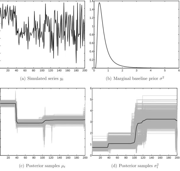
We simulate a time series ofT = 200observations from a process with three regimes in both mean and variance, where the structural breaks occur at t = 40 and 100. Figure 2(a) shows the simulated time series. After employing the Gibbs sampler with the remix step for 2,000 runs, we obtain the posterior time paths for µ and σ2
as depicted in Figures 2(c)–(d), where the first 1,000 runs are discarded as burn-in and only the last 1,000 runs are used for constructing the posterior distributions. The chain converges quickly and this only requires 1-2 minutes computing time on a modern personal computer. We see that the data generating process is accurately retrieved and the imposed simultaneous breaking of the two parameters is not restric-tive. Figure 2(b) shows the marginal baseline prior for σ2. Since we have a regime
with variance equal to 4 and the baseline prior has only modest support for values larger than 2, it is interesting to note that the variance of this volatile regime is still properly estimated. However, this remark is certainly something to be aware of while choosing the baseline distribution. We further address this issue in the illustrations in Section 4.
The above derived Gibbs sampler can be applied to conjugate and conditional conjugate settings. That is, in case of independent breaks in a vector of time-varying parameters, where we have multiple layers as in (1), we can condition on other time-varying parameters and still employ this procedure.
3.1.2 Non-conjugate setting
In the case of non-conjugate baseline priors and likelihoods we propose to implement a Metropolis–Hastings [MH] sampler. Instead of direct sampling from the consecu-tive full conditional posteriors, we now use the full conditional priors as candidate distributions to obtain the following algorithm:
Step 1. Initialize the vector of time-varying parameters10 at θ(1); set m = 1 and
repeat Step 2 form = 2, . . . , M (= number of simulation runs);
Step 2. For t = 1, . . . , T sample from the full conditional prior as in (4) and use this proposal valueθ#t as a sample from the candidate distribution. The result
in (9) determines the MH-steps:
• Compute the proposal acceptance probability (which is the ratio of one-observation likelihoods) α(θt(m), θt#) = min pyt|y1,t−1, θ#t pyt|y1,t−1, θt(m) ,1 ;
• Set θ(tm+1) =θt#with probabilityα(θ
(m) t , θt#) andθ (m+1) t =θ (m) t otherwise.
Because of the assumption that structural breaks occur only infrequently, the full conditional prior is the dominant part in (9). Exactly this makes the chosen can-didate distribution a well-performing option. Moreover, for the large majority of the observations there will be no break and in iteration m it will hold that
θ(t−m1) = θ(tm) = θ(t+1m) ≡ θ∗. In this case the proposal value θ#
t will very likely be
θ∗ and no likelihood evaluations at all are needed as the acceptance probability
obviously equals one. Hence, this MH-sampler requires even less computations com-pared to the previous Gibbs sampler and is stillO(T). However, because π is small, convergence may take longer. Starting with a no-breaks situation it may take a while before the non-degenerate component f0 is sampled from.
For the remixing in (11) we can sample from a close candidate and perform an MH-step or, for low-dimensional cases, implement a griddy-Gibbs step (see Ritter and Tanner; 1992).
10The easiest way to do so is simply starting in a case of no breaks at all, that is, setθ(1)
t =θ0,
3.2
Baseline parameters
In case of a prior on the hyperparameters of the baseline distribution, we can update by extending the discussed simulation scheme as in any hierarchical model. Condi-tional on θ we can construct the vector of the K unique parameter values θ∗ that are independent draws fromf0(θk∗;λ). Therefore, updating λ means sampling from
p(λ|y,θ∗) ∝ p(λ)
K
Y
k=1
f0(θ∗k;λ). (12)
Clearly, a conjugate prior distribution for λ usually facilitates this simulation step. We refer to Section 4 for examples.
3.3
Breaking probability
In case we treat the probability of a break π as an unknown parameter, we can include it in the MCMC simulation scheme and update by simulating from its full conditional posterior, which can be written as
p(π|y,θ) ∝ p(π)
T
Y
t=2
p(θt|θt−1),
because the conditional densities of the parameters are the only parts that involve
π. Conditional on a sampled value of the parameter vector, the transition densities reduce to
p(θt|θt−1) =
(
πf0(θt), if θt 6=θt−1,
πf0(θt) + (1−π), if θt =θt−1.
This shows that a Beta prior does not automatically lead to a full conditional distri-bution which is also Beta, as the termπf0(θt) in caseθt=θt−1 does not cancel out.11
However, we can augment the parameter vector with a vector of indicator variables s= (s2, . . . , sT)0, such that conditional on these indicators π can be sampled from a
Beta distribution, see Geweke and Jiang (2010) and their specification in Section 2.1. Sampling sconditional onθ is simple and fast. Importantly, given θ the st’s are
non-degenerate. We refer to Appendix B for details of this step and for a proof that it leads to the proper invariant distribution. Note that we actually twist the procedure
11Becauseπf
0(θt) is small it is very close to a Beta distribution. Applying an MH-step with as
proposed by Giordani and Kohn (2008). Instead of simulating indicators and states in one block by integrating out the states first, we sample in one block by first analytically integrating out the indicator variables. This results in a computationally more attractive way to do inference.
If we now take a Beta prior for π the full conditional posterior (conditional on s) ofπ is also Beta:
π∼ Be(r1, r2) =⇒ π|y,s∼ Be(K∗+r1, T −1−K∗+r2),
with K∗ = PT
t=2I{st=1} which is larger than or equal to the number of in-sample
breaks K−1.
4
Illustrations
In this section we demonstrate the practical usefulness of our approach by presenting four illustrative applications. As we want to highlight the general applicability of our approach to different types of time series models, the illustrations involve a Poisson count data model, a copula model, a probit model and an autoregressive model. These four examples will touch on issues relevant with respect to the modeling process and estimation, including prior specification and the computational ease of our approach in nonlinear models.
4.1
A Poisson count data model for earthquake data
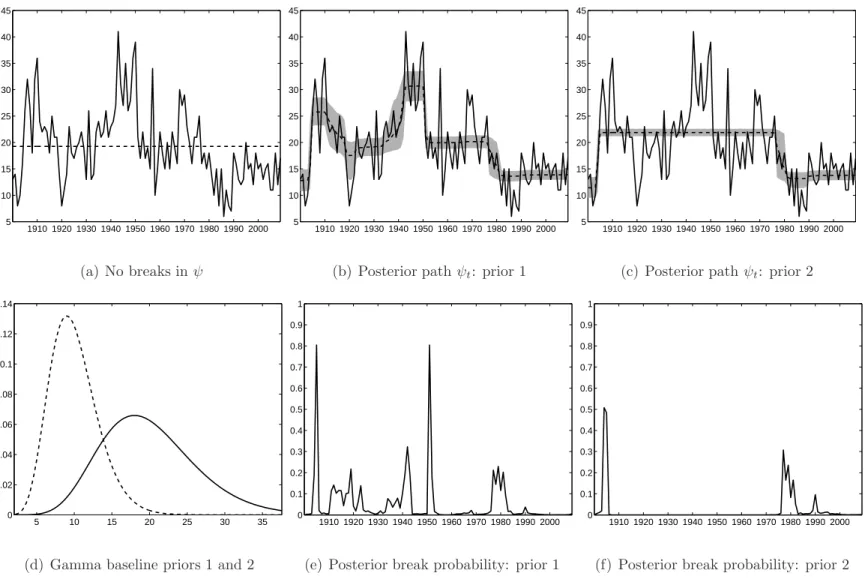
In this example we investigate possible structural instability in a count data model, that is, a model for a time series that takes only discrete values within a limited range. Specifically, we consider a Poisson model for describing the worldwide annual counts of extreme earthquakes (larger than 7.0) for the period 1900-2009.12 The time
series is displayed in Figure 3(a), showing that it ranges between a minimum of 6 in 1986 and a maximum of 41 in 1943. It also appears that the series may be subject
12Taken from the Time Series Data Library by Rob Hyndman: Hyndman,
R.J. (2010), http://robjhyndman.com/TSDL accessed on July 23, 2010. Orig-inally collected by the National Earthquake Information Center, which source (http://earthquake.usgs.gov/earthquakes/eqarchives/year/eqstats.php) we also have used to extend the sample with data up to 2009.
to occasional level shifts. We examine this possibility by allowing for time-variation in the mean parameter of the Poisson model. The complete model is given by
yt|ψt i.i.d.
∼ Poi(ψt),
p(ψt|ψt−1) = πf0(ψt) + (1−π)I{ψt=ψt−1}, f0(ψ) = fGa(ψ;a, b).
where we opt for a Gamma baseline prior for the parameterψ to obtain a conjugate setting.
This conjuage setting implies that we can implement a straightforward Gibbs sampler for this model. The necessary marginal likelihoods become
p0(yt) = ba (b+ 1)a+yt Γ(a+yt) Γ(a)yt! ,
where the ratio on the right reduces to a+yt
a
if a is integer. The one-observation posterior for the continuous mixture component is
ψt|yt ∼ Ga(a+yt, b+ 1).
Naturally, the posterior for the remix step, conditional on the breaking dates is
ψk∗|y(k) ∼ Ga a+Xtk t=tk−1+1 yt, b+ (tk−tk−1) ,
where k denotes the regime.
Posterior results for this model are depicted in Figure 3. The results are based on 5,000 iterations of the Gibbs sampler of which the first 2,000 iterations serve as burn-in. This takes about 2-3 minutes computing time. In Figures 3(b)–(c), we display the posterior marginal distributions of theψt’s for two different parameterizations of the
Gamma baseline prior. The density functions of these two baseline priors are given in Figure 3(d). If we choose for a relatively uninformative prior with wide support, three distinct kinds of geophysical activity seem to occur. If we choose for the more restrictive prior with support concentrated under 20, the ‘high-activity’ type (values around 25-30) is not present anymore, see Figure 3(c). This demonstrates that it is important that the prior onψ has enough support to capture all possible regimes in the data. Figures 3(e)–(f) show the marginal posterior break probabilities for each point in time. These are Pr[ψt 6= ψt−1|y] = EI{ψ
t6=ψt−1}|y
can easily be computed using the Gibbs output by simply counting the number of breaks given a sample of ψ1,T from the posterior. The probabilities in Figures 3(e) indicate that the structural breaks may either occur almost instantaneously (as in 1905 and 1951) or gradually (during the 1910s, the late 1930s and early 1940s, and around 1980).
4.2
Breaks in copula model parameters
To illustrate the usefulness of our approach in non-conjugate settings we examine a copula model, which is becoming increasingly popular in empirical finance to capture non-standard cross-sectional dependence (see, for example, McNeil et al.; 2005; Jondeau and Rockinger; 2006). We simulate 400 observations ut= (u1t, u2t)0,
(t = 1, . . . ,400), from a bivariate Clayton copula, given by C(ut;θt) = (u−1tθt +
u−θt
2t −1)−1/θt, with θt>0. The parameterθtdetermines the strength of dependence
betweenu1tandu2t, with higher values indicating stronger dependence. For example,
Kendall’sτ is equal to θt/(θt+ 2). Furthermore, the Clayton copula is characterized
by lower tail dependence and upper tail independence, in the sense that lim q↓0 Pr[u2t≤q|u1t≤q] =C((q, q)0;θt)/q= 2−1/θt, lim q↑1 Pr[u2t≥q|u1t≥q] = [1−2q+C((q, q)0;θt)]/(1−q) = 0.
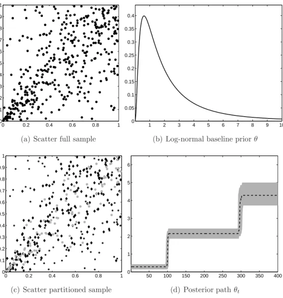
We impose three regimes with structural breaks occurring at observations 101 and 301. The copula parameter values for these three regimes are 0.1, 2 and 5, re-spectively. Figure 4 displays some characteristics of the simulated data. Figure 4(a) shows a scatter of the bivariate data over the whole sample period in the unit square. No structural change is visible at first sight. Figure 4(c) displays the same data but here we distinguish between the three regimes by using different marker types. For example, the grey bullet data correspond to the most recent regime in whichθ = 5; the large parameter value implies stronger (left-tail) dependence.
We use the following model to estimate the parameters of the Clayton copula for the simulated series:
ut|θt i.i.d.
∼ CCl(θt),
p(θt|θt−1) = πf0(θt) + (1−π)I{θt=θt−1},
The log-normal baseline prior exhibits desirable properties as it can be used for any parameter which is bounded from below/above. It is easy to see that the baseline prior f0 and the likelihood cCl(ut|θt) =∂2C(ut;θt)/(∂u1t∂u2t) are non-conjugate, so
we have to use the Metropolis-Hastings sampler to simulate from the full conditional posteriors p θt|U,θ[−t]
with U = (u1, . . . ,u400)0. For the remixing step we use a
griddy-Gibbs step where we take into account thef0-prior for the regime parameter:
θ∗
k ∼logN(a, A), (k = 1, . . . , K).
If θ ↓0 the Clayton copula becomes an independent copula. The first regime is close to this situation. Therefore we consider a quite uninformative baseline prior (a= 0.5 andA = 1) which also covers values close to zero. The density of the prior is depicted in Figure 4(b). As we expect only a few breaks we set π equal to 0.01. Posterior results are shown in Figure 4(d). It turns out that the marginal posteriors of the parametersθt resemble the data generating process closely. We see very sharp
and sudden shifts in the parameter value at times t = 101 and t = 301. Posterior results turn out to be quite robust with respect to prior parameters settings and specification of the baseline prior. The computational burden of our approach is small as it takes only three minutes computing time to obtain 3,000 draws from the posterior distribution.
4.3
Size spread sign prediction
In the third illustration we apply our method to a probit model to forecast the sign of the size spread in monthly U.S. stock returns. The size spread is defined as the difference between the returns on portfolios consisting of the 20% smallest stocks and portfolios consisting of the 20% largest stocks over the period July 1962 - October 2010.13 Hence, the data correspond to binary random variables y
t, which equal 1 if
the difference is positive and zero otherwise. We model these binary variables using a probit specification:
yt|xt,βt i.i.d.
∼ Ber(Φ(x0tβt)), (13)
where Φ(·) is the CDF of the standard normal distribution. For the explanatory variables xt we use a number of series that are typically considered for predicting
13The data were obtained from Kenneth French’s website data library
(relative) stock returns. A preliminary analysis suggests to use the following five variables: credit spread, term spread, market return, and the growth in the Con-ference Board’s leading index.14 We also include an intercept and the one-month
lagged size spread. As empirical studies indicate that the relation between some of the explanatory variables and stock returns change (see, for example, Pesaran and Timmermann; 2002), we allow for breaks in theβ parameters.
Since we are dealing with a simple 0/1-series, we must be careful not to demand too much from the data. For example, allowing all six parameters to vary leads to too much flexibility corresponding to perfect fit in some time periods.15 Therefore
we focus on possible changes in the effect of the two spread variables and we only allow their coefficients, βCS and βTS, to change simultaneously over time. Thus, we
extend the model in (13) with the conditional distribution
p(βS,t|βS,t−1) =πf0(βS,t) + (1−π)I{βS,t=βS,t−1},
and we propose to use the following Gaussian baseline prior:
βS = (βCS, βTS)0|µ,Σ ∼ N(µ,Σ). (14)
For the time-invariant part of βt we apply an uninformative conjugate Gaussian
prior. As discussed before, especially for forecasting purposes it would make sense to update the hyperparameters of the baseline prior. We consider a matricvariate normal-inverted Wishart prior for the hyperparamters:
µ0|Σ ∼ MN(p0, q·Σ), (15) Σ ∼ IW(S, u). (16)
For the breaking probability π we take a Beta prior with parameters r1 and r2.
14To be more precise: (1) credit spread: the difference between Moody’s Baa corporate bond rate
and the 10-year Treasury constant maturity rate, in deviance from its one-year moving average; (2) term spread: the difference between the 3-month Treasury bill secondary market rate and the effective Federal funds rate, in deviance from its one-year moving average; (3) stock market return: level of the S&P500 index relative to a two-year moving average; (4) growth in leading index: growth rate of The Conference Board’s Composite Leading index over the six most recent months. All explanatory variables are available at the actual time the forecast is constructed, that is, some of them are appropriately lagged to take into account publication delays.
15This issue becomes even more relevant when the data show persistent clustering of zeros or
The prior hyperparameters are set to p0 = (0,0), q = 2, S = 2·I
2 and u = 6.
Following the suggestions in Giordani et al. (2007) the parameters of the prior forπ
are set to r1 = 5, r2 = 3000, which corresponds to a prior assumption of one to two
breaks. Because of the non-conjugate setting of (13) and (14) we have to rely on the MH-procedures described in Section 3.1 to sample from the posterior distribution.16
To speed up convergence of the chain we employ a tailored remix step. For the remix step we sample latent variables from truncated normals just as in an MCMC sampler for a probit model based on data augmentation (see, for example, Albert and Chib; 1993). Conditional on these latent variables we resample the βS parameters. Note
that we only use these variables for the remixing step.
Figure 5 shows the posterior results of this sampler based on 7,000 iterations of the MCMC sampler of which the first 2,000 serve as burn-in. Figures 5(a) and (c) show the posteriors of the two parameters that may be time-variant. Initially the credit spread has no impact, but since the late 1970s its effect becomes positive. After the end of the 1990s the effect becomes negative. The term spread has a positive impact from the beginning of the sample which becomes even stronger in the early 1980s, though, its posterior uncertainty also increases.
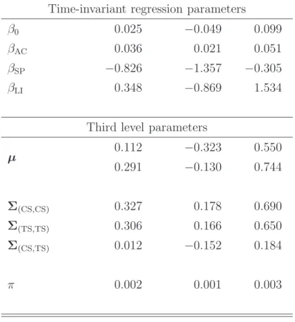
The marginal properties of the posterior distribution of the model parameters are reported in Table 1. The posterior median of the µ parameters is larger than the median of the prior although the increase is small due to the fact that we only have a small amount of breaks in the sample. Figure 5(b) shows the posterior of the two marginal baseline densities implied by f0(·;µ,Σ) integrated over the posterior
p(µ,Σ|y). The posterior baseline belonging to the term spread is slightly more shifted to the right due to the positive effect of the term spread on the size spread sign.
In Figure 5(d) we show the ‘fitted’ in-sample probabilities; Φ(x0
tβt) integrated
over the posterior distribution. These probabilities do not show an outspoken pattern which is inherent to these models. The hitrate is 63% based on a cut-off of 0.5.
16If we use data augmentation for the probit part we can rely on Gibbs steps but this extends
4.4
Forecasting U.S. quarterly GDP growth
Our final illustration examines structural breaks in an AR(4) model for quarterly growth in U.S. gross domestic product and the implications with regard to forecast-ing. Similar exercises have been employed by McConnell and Perez-Quiros (2000); Clark (2009) and Geweke and Jiang (2010), for example. If yt is the annualized
quarterly growth rate for the sample period 1960Q1-2010Q3 and the random shocks are assumed to be Gaussian, then the standard AR(4) representation can we written as yt=αt+ξtyt−1+ 3 X j=1 ϕ∗j∆yt−j+εt, εt i.i.d. ∼ N 0, σt2 ,
where we condition on the observations before 1960Q1.
First, we allow for infrequent intercept shifts and changing persistence through the conditional mean parameters αt and ξt, respectively. We impose simultaneous
changes in these two parameters to control for the fact that the unconditional ex-pectation ofytis determined by both in a positive way. A shift in the unconditional
mean, either through the intercept or the persistence parameter occurs with proba-bility π1. To impose unit root stationarity ξt should take values smaller than 1. In
our framework this truncation is easily dealt with. Further (conjugate) considera-tions lead to a truncated multivariate Gaussian baseline prior distribution for the time-varying mean parameters θt= (αt, ξt)0:
p(θt|θt−1) = π1f0(θt) + (1−π1)I{θt=θt−1},
θ|µ,Σ ∼ N(µ,Σ)×I{ξ<1}. (17)
Shifts in the volatility of the random shocks (σ2
t =Var[εt|σ2t]) are modeled
inde-pendently from the previous regression parameters. Therefore we specify a separate layer as in (1) with a break in variance occurring with probability π2. For this
parameter we opt for an inverted Gamma–2 baseline prior:
p(σt2|σ2t−1) = π2f0(σt2) + (1−π2)I{σ2 t=σt2−1}, σ2|Ω, ν ∼ IG2(Ω, ν).
In order to update the baseline prior parameters, we augment the model with a third level. For the baseline parameters of the truncated Gaussian in (17) we use the same conjugate choice as in the sign prediction model of Section 4.3, see
(15)–(16). Following Clark (2009), we use the pre-sample data to set its parameters p= (2,0.4)0,q = 10,u = 6 and S= 2·I2.
We impose an inverted Gamma–2 prior for the parameter Ω of the baseline distribution of the conditional variance. This allows us to learn with respect to the distribution of σ2
t:
Ω∼ IG2(W, z).
To simulate Ω during the MCMC scheme we implement an independence MH-simulator with a Gamma distribution to generate proposal values. Again we use historical data and take W = 50, z = 6 andν = 9.
Further prior settings involve a conjugate Gaussian prior on the time-constant parameters
(ϕ∗1, ϕ∗2, ϕ∗3)0 ∼ N(b,B),
where we set its hyperparameters such that it is close to a flat prior. To complete, since we have two layers that account for structural breaks in the mean parameters and the conditional variance, respectively, we have to set two priors for the associated break probabilities π1 and π2. We use two independent Beta priors:
π1 ∼ Be(r11, r12) and π2 ∼ Be(r21, r22),
and we set r11 = 5, r12 = 1000, r21 = 1 and r22 = 100. This way the expected
probability of a break in either the mean or the conditional variance is approximately equal to 0.02.
The assumption of independence between the two layers has the following im-plications for estimation. Conditional on the standard deviations σ = (σ1, . . . , σT)0,
we have a conjugate setting17 and therefore we can employ the Gibbs sampler to
simulate (αt, ξt)0, (t = 1, . . . , T). Vice versa we also have a conjugate setting and
can simulate the conditional variances.
Figures 6(a) and (d) show the data and the posterior unconditional mean of
yt, and the posterior path of σt2, respectively. The unconditional mean is given by
αt/(1−ξt). Figure 6(a) shows that no shifts have occurred during the sample period;
α is in the range [1,1.9] and the persistence parameterξ covers values in [0.4,0.65].
17Even with the truncation of the Gaussian baseline prior for ξ, the marginal likelihoods and
posterior distributions can be obtained analytically. Of course, the MH-routines can be applied equally well.
The variance does show significant changes, in line with previous empirical findings. The Great Moderation corresponds to the large decline in volatility in the early 1980s. Recent negative growth rates suspect this decline is being offset, see Clark (2009). However, more data are needed to provide more strong evidence in favor of this hypothesis.
In Figures 6(b) and (c) we display the evolution of the marginal posterior pre-dictive distributions p(yτ+h|y1,τ) for h = 1, . . . ,40, for two cases: no breaks at all
and the previously described structural break model, respectively. Forecasting starts at τ = 2002Q4. Figures 6(e) and (f) show the marginal posterior predictive densi-ties for horizions one quarter ahead (solid) and ten years ahead (dashed). Clearly, if we assume parameter stability the Great Moderation is not accounted for and the current variance is heavily overestimated leading to too wide density forecasts. The structural break model starts with tighter forecast densities due to the smaller estimated σ2
τ. If the forecasting horizon grows, we see that incorporating future
structural breaks leads to a predictive distribution that is more peaked than the Gaussian in Figure 6(e). This heavy-tailedness assigns more probability mass to more extreme values as realized in 2010.
5
Conclusion and discussion
In this paper we have proposed a dynamic stochastic specification to model infre-quent sudden changes in model parameters over time. The specification is simple and has many nice desirable properties.
First of all, the number of in-sample and out-of-sample breaks and the break dates are a priori unknown. The dynamic specification contains natural implications in terms of out-of-sample forecasting. In existing models, future parameter breaks are neglected or require (computationally demanding) extensions. Our approach implies a random number of out-of-sample breaks where its distribution depends on the fore-casting horizon and the breaking probability. The risk of future breaks is assimilated in the posterior predictive distributions according to the rules of probability.
Second, our approach is flexible in the sense that the posterior simulator does not impose any restrictions on the model under consideration. Hence, we do not have to limit ourselves to linear regression models or models which can be written in