Wild adaptive trimming for robust estimation and
cluster analysis
ANDREA
CERIOLI
†,
ALESSIO
FARCOMENI
‡,
MARCO
RIANI
††
Department of Economics and Management, University of Parma
‡Department of Public Health, Sapienza - University of Rome Italy
Abstract
Trimming principles play an important role in robust statistics. However, their use for clustering typically requires some preliminary information about the con-tamination rate and the number of groups. We suggest a fresh approach to trim-ming that does not rely on this knowledge and that proves to be particularly suited for solving problems in robust cluster analysis. Our approach replaces the original
K-population (robust) estimation problem withKdistinct one-population steps, which take advantage of the good breakdown properties of trimmed estimators when the trimming level exceeds the usual bound of 0.5. In this setting we prove that exact affine equivariance is lost on one hand, but on the other hand an arbi-trarily high breakdown point can be achieved by “anchoring” the robust estimator. We also support the use of adaptive trimming schemes, in order to infer the con-tamination rate from the data. A further bonus of our methodology is its ability to provide a reliable choice of the usually unknown number of groups.
Key words: Breakdown Point; Forward Search; MCD; Outliers; Robust Clustering
1
Introduction
Trimming principles play an important role in robust statistics and allow to solve com-plex problems in the analysis of contaminated multivariate data (see, e.g., Clarke and Schubert, 2006; Cuesta-Albertos et al., 2008; Garc´ıa-Escudero et al., 2008; Ritter, 2014; Farcomeni and Greco, 2015). LetX = {x1, . . . , xn} be a random sample
ofv-variate observations from a population with distribution functionG(x). We as-sume thatG(x) is an unknown element within a familyG of distribution functions such that
G={G(x) :G(x) = (1−ǫ)G0(x) +ǫG1(x); x∈Rv; ǫ∈[0,1)}, (1) whereG0(x) is the distribution function of the “good” part of the data, i.e. G0(x)
to a classCof distributions andǫis the contamination rate. Although it is not necessary to defineCas a specific parametric family, some regularity conditions on it are often assumed (see, e.g., Cuesta-Albertos et al., 2008; Cerioli et al., 2013).
In the one-population version of model (1) it is common to take
G0(x) = Φµ,Σ(x), (2)
whereΦµ,Σ(x)is the distribution function of av-variate normal random variable with
meanµand dispersionΣ. The trimmed estimators ofµandΣtake the form
˜ µα= 1 Wα n X i=1 wi,αxi, (3) ˜ Σα= ζα Wα n X i=1 wi,α(xi−µα˜ )(xi−µα˜ )′, (4) whereα∈(0,0.5), eitherwi,α= 0orwi,α= 1,Wα=Pn
i=1wi,α, and ζα= 1−α Gχ2 v+2(χ 2 v,1−α) (5)
is a scaling factor ensuring consistency ofΣ˜αwhenǫ= 0. In (5), we defineGχ2
v(·)to be the distribution function of aχ2
vrandom variable, while χ2v,1−α=G−χ21
v(1−α) (6)
is its(1−α)-th quantile. Computation of the binary weightswi,α, i = 1, . . . , n, is sketched in§2.1 and§2.2 for two alternative trimmed estimators. In all cases, the weightswi,α are defined in such a way thatWα = ⌊(1−α)n⌋, where⌊·⌋denotes the floor function. The numberαthus gives the trimming level, i.e. the proportion of observations discarded by the robust procedure. The squared distances
di,α2 = (xi−µα˜ )′Σ˜α−1(xi−µα˜ ) i= 1, . . . , n (7)
are used for outlier identification and, more generally, for robustly ordering multivariate data (Atkinson et al., 2004; Hubert et al., 2008; Riani et al., 2009; Cerioli, 2010).
In the standard approach to trimmingαmust be fixed in advance, thus requiring some a priori information on the degree of contamination in model (1). Otherwise, the usual suggestion is to chooseα=ǫ∗−1/n, where
ǫ∗=⌊(n−v+ 1)/2⌋/n≈0.5 (8) is the maximal value of the (replacement) breakdown point ofµα˜ and Σ˜α (Davies,
1987; Lopuha¨a and Rousseeuw, 1991). Under model (1), this choice corresponds to the assumption that at least50%plus another⌈(v−1)/2⌉observations, where⌈·⌉is the ceiling function, come fromG0(x), i.e. that
ǫ < 1
Condition (9) is very natural in one-population models forG0(x), like (2) (see, e.g.,
Rousseeuw and Leroy, 1987, p. 14). However, choosingα= ǫ∗−1/nmakes
com-putation of the trimmed estimatorsµα˜ andΣ˜α virtually useless when there is more
than one “good” population and the goal is to robustly cluster the observations inX according to these populations. In a multi-population structure forG0(x), we typically
assume that the “good” data come from
G0(x) = K X k=1 πkΦµk,Σk(x), πk>0, K X k=1 πk= 1, (10) whereK is the unknown number of populations,µk andΣk are population-specific
parameters, andπ1, . . . , πKare the unknown mixing proportions. It is then possible to
identify the largest population inG0(x)through estimates (3) and (4), and the
associ-ated robust distances (7), only in the unlikely situation wheremaxkπk≫0.5. Indeed,
a simple example where trimming methods fail to detect a multi-population structure even ifmaxkπk ≈0.6is provided by Atkinson et al. (2004, pp. 372–373). A related
qualitative comment is made by Huber and Ronchetti (2009, p. 21).
The goal of this work is to suggest a fresh approach to trimming that allows com-putation of the trimmed estimatorsµα˜ and Σ˜α also whenG0(x) follows (10) with maxkπk≤0.5. Our methodology is particularly suited for solving problems in robust
cluster analysis, whose aim is to identify individual membership to the populations that originate mixture (10). This is achieved by replacing aK-population (robust) es-timation step, at the heart of the available model-based clustering algorithms, withK
distinct one-population steps, which take advantage of (3) and (4). Specifically, our proposal consists in computing the trimmed estimatorsµα˜ andΣ˜αwithα≥0.5, and
possibly much larger than the usual bound(ǫ∗ −1/n). We name our method wild
trimming, since we suggest to trim much more than it is customary following (8).
In-deed, our trimming level can be as large as the highest value ofαfor which Σ˜α is
positive definite. We also strongly support the use of adaptive procedures (in the sense described by Huber and Ronchetti, 2009, p. 8), where the trimming level is not fixed in advance, but different values ofαare used and the best one is selected from the data, thus yielding a closer agreement betweenαin (3) and (4), andǫin (1). Therefore, the output of our methodology is a robust procedure where not all units inX are clas-sified into groups, since we discard the observations that are believed to come from the contaminant distributionG1(x), and where neither the number of groupsK nor the
trimming levelαare specified a priori.
In spite of its simplicity, we believe that the idea behind wild trimming has not gained the popularity that it deserves. One motivation lies in the often implicit assump-tion that the “good” populaassump-tion should correspond to the majority of data. Instead, our point of view is different and we define outlyingness of a multivariate observation with respect to a specific point, sayx0, ideally sampled fromG0(x). In our framework also
the bulk of the data can become anomalous if sufficiently far fromx0. Wild trimming
thus provides a very natural approach, since condition (9) is not required. Although the robustness properties of the estimators obtained withα ≥ 0.5 turn out to be far from trivial, they are intuitively appealing and obviously do not contradict the well known findings for the caseα <0.5, such as the fundamental bound (8). One
excep-tion towards the applicaexcep-tion of wild trimming ideas is provided by the Forward Search, which has shown good potential for performing robust cluster analysis (Atkinson et al., 2004, 2017), but mainly in an exploratory context. Our work thus puts robust cluster-ing through the Forward Search within a statistically principled framework where the robustness properties of the algorithm are made explicit. However, our goal is more ambitious and through our methodology we aim at performing robust estimation and cluster analysis under the same umbrella, with data-driven selection of bothKandα. This task is clearly not possible in the standard approach to trimming, whereα <0.5, and is also problematic through the available robust clustering techniques, which re-quire some a priori information about the features of models (1) and (10).
The paper is structured as follows. In§2 we introduce the two multivariate trimmed estimators that we use in our work. In§3 we obtain the robustness properties of these estimators under wild trimming and we define a new class of estimators having the required breakdown properties. The suggested robust divisive clustering method is detailed in§4. We show the practical advantages of our proposal in§5, where we also provide comparisons. Some concluding remarks are given in§6. Further examples are provided in the Supplementary Material.
2
Multivariate (adaptive) trimming
2.1
The Minimum Covariance Determinant
For trimming levelα, the Minimum Covariance Determinant (MCD) subset ofX is defined as the subsample ofhα =⌊(1−α)n⌋observations whose covariance matrix has the smallest determinant. Letι♭
α ={i1, . . . , ihα}denote the set of the indices of the observations belonging to this subset. The MCD estimators ofµandΣ(Rousseeuw and Leroy, 1987, p. 262–265) are then defined by (3) and (4), with weights
wi,α = 1 if i∈ι♭α (11)
= 0 otherwise,
andWα =hα. The MCD estimators are consistent under very general conditions on
G(x)(Butler et al., 1993; Cator and Lopuha¨a, 2012). They also attain the breakdown bound (8) whenα = ǫ∗−1/n. To increase efficiency, while keeping a high
break-down point, a one-step reweighting scheme is often used. Reweighted estimators are computed by giving weight 0 to observations for which the squared robust distance (7) exceeds a threshold value, defined in terms of a new trimming levelα∗ ∈ (0, α)and
such thatα∗≪α. The reweighted MCD (RMCD) estimates are then obtained through
(3) and (4), but now with weights
wi,α∗ = 1 if d2i,α≤d2α∗ (12)
= 0 otherwise,
and scaling factorζα∗ = (1−α∗)/{Gχ2
v+2(χ
2
v,1−α∗)}. A popular choice in (12) is
α∗ = 0.025, so thatd2
α∗ is the(1−α∗) = 0.975-th quantile of the distribution of
consideredd2
α∗ =χ2v,0.975, but more accurate approximations exist (Hardin and Rocke,
2005; Cerioli, 2010). The RMCD estimates can thus be seen as the result of a two-step adaptive trimming procedure, computed using two different subsets ofX. Each of these subsets is defined by a specific trimming level: αin the initial step andα∗ in
the reweighting stage. An advantage is that the number of units declared to be outliers by distances (7), and thus discarded in the second subset, can provide information on the contamination rateǫin model (1). A fully adaptive procedure based on the MCD should extend the reweighting scheme to a decreasing sequence of trimming levels, starting fromα, and monitor the resulting changes in the parameter estimates (see Riani et al., 2014; Cerioli et al., 2017). A similar approach is exploited in the Forward Search.
2.2
The Forward Search
The Forward Search (FS) is a flexible general method for detecting anomalies in struc-tured data (Atkinson et al., 2004). Given a sample ofnobservations and a generating model for them, the method starts from a subset of cardinalitym0 ≪n, which is
ro-bustly chosen to contain observations coming from the postulated model. This subset is used for fitting the model and suitable deviance measures are computed. The subse-quent fitting subset is then obtained by taking them0+1observations with the smallest
deviance measures. The algorithm iterates this fitting and updating scheme until all the observations are used in the fitting subset, thus yielding the classical statistical sum-mary of the data. Therefore, the FS applies a decreasing sequence of trimming levels
α0> α1> . . . > αL>0, with α0= 1−m0 n , (13) αl=αl−1− 1 n, l= 1, . . . , L, (14)
andL = n−m0. Clearly, αL = 1/n, while in the last step of the FS we have
αL+1=αL−1/n= 0and no trimming is performed. The typical initialization in a
multivariate framework is withm0=v+ 1observations in (13), so thatL=n−v−1.
A slightly larger value ofm0is sometimes selected to improve numerical stability of
the initial estimates.
At stepl = 1, . . . , Lof the FS, the trimmed estimators (3) and (4) are computed with weights wi,αl = 1 if i∈ι † αl (15) = 0 otherwise, whereι†
αl={i1, . . . , iml}is the set of the indices of theml=⌊(1−αl)n⌋observations that form thel-th fitting subset. Specifically,ι†
αl is obtained by taking the units with themlsmallest squared distances
d2i,αl−1= (xi−µα˜ l−1)
′Σ˜−1
computed from the estimates with trimming levelαl−1. The initial setι†α0, of
cardi-nalitym0 =⌊(1−α0)n⌋, is instead defined through an exogenous criterion, such as
the intersection of robust bivariate projections, or the optimization of a robust objective function on subsets ofm0 observations. In§4 we adopt a random sampling strategy
that proves to be suitable for clustering purposes.
The presence of observations deviating from the null model can be displayed through pictures that monitor relevant quantities along the search, such as the squared robust distances (16) and their order statistics. For instance, if onlyn0 < n units actually
belong to the postulated population, we typically observe a peak in the monitoring plot of the minimum (squared) distance outside the fitting subset, when this subset only contains then0“good” observations and the first outlier is about to enter. A formal
procedure for precise identification of the contaminated observations is developed by Riani et al. (2009) when (2) is the null model. Under the same assumption, Cerioli et al. (2014) show that the FS estimators are both consistent and robust, while Johansen and Nielsen (2016a,b) provide a general asymptotic theory for the FS in regression.
3
Robustness properties under wild trimming and a new
class of estimators
Unless otherwise stated, in what follows we make use of the replacement version of the breakdown point (BP) of an estimator, which is defined as the smallest fraction of outliers that can take the estimate over all bounds. A well known result of Lopuha¨a and Rousseeuw (1991, Th. 2.1) is that the maximal BP of any translation equivari-ant location estimator cannot exceed⌊(n+ 1)/2⌋/n. An estimator of locationt(·)
is translation equivariant ift(x+c) = t(x) +c. Instead, we say that an estimator is quasi-translation-equivariant if it is translation equivariant within a subspace (see Proposition 2 below).
The result of Lopuha¨a and Rousseeuw (1991) corresponds to the intuitive statement that we should trim at most a portionα = ⌊(n−1)/2⌋/nof the observations, in order to get rid of the possible contaminants and to base our estimate on a subset of at least⌊n/2⌋+ 1“good” data points. However, in this paper we use trimming levels much larger than 50% and it is natural to wonder what are the breakdown properties of our location estimators. There are only two possibilities: either our estimators are translation equivariant and their BP is⌊(n+1)/2⌋/neven if the trimming level is much larger than⌊(n−1)/2⌋/n, or they can achieve a BP much larger than 50% but they are not translation equivariant. The latter claim holds. Formally, we define a class of trimmed quasi-translation-equivariant location estimators whose breakdown point can be arbitrarily higher than 50%, depending on the chosen level of trimming.
To do so, we fix a point x0 ∈ Rv. We define an anchored class of estimators,
saytx0(·), which correspond to the original MCD (or FS, or other trimmed) estimator.
of the location parameterµfor trimming levelαis then tx0(X) = 1 ⌊n(1−α)⌋ ⌊n(1−α)⌋ X i=1 x‡i, (17) wherex‡⌊n(1−α)⌋ = {x‡1, . . . , x ‡
⌊n(1−α)⌋} is the minimizer of the objective function
among all the subsets of⌊n(1−α)⌋points ofX whose convex hull containsx0. We
remark that in this paper we indicate with the term “objective function” the objective function of any estimator of interest, be it MCD, or any another high-breakdown mul-tivariate estimator (excluding FS which involves a sequence of selection steps); and with the term “solution” to the objective function the estimator itself. The anchored estimator arises as a solution to an anchored objective function, that is, a constrained objective function that we now formally define. Specifically, we look for solutions of the objective function subject to
∃(λ1, . . . , λ⌊n(1−α)⌋) : λi≥0 and ⌊n(1−α)⌋ X i=1 λi= 1 and||x0− ⌊n(1−α)⌋ X i=1 λix‡i||= 0, (18) for a norm|| · ||.
Some results for anchored trimmed estimators follow. A key issue in their deriva-tion is that any point within the support ofG0(x)also belongs to the convex hull of the
points in the support. Additionally, convex hulls are non-decreasing: for every two sets
AandB, whereA⊆B, the convex hull ofAis a subset of the convex hull ofB.
Proposition 1 Ifx0belongs to the convex hull of the points inX, the anchored trimmed
estimator exists. Ifx0belongs to the interior of the support ofG0(x), the probability
that the anchored trimmed estimator of location exists converges to the unity with the sample size.
Proof. By the non-decreasing property of convex hulls, the convex hull of any subset of
size⌊n(1−α)⌋is a subset of the convex hull ofX. Consider the set of all subsets of size⌊n(1−α)⌋and callhjthe convex hull of thej-th subset, andhthe convex hull of X. It is straightforward to check that∪hj⊆h. Therefore, ifx0belongs to the convex
hull ofX, there must exist at least one subset of size⌊n(1−α)⌋whose convex hull containsx0. To see the second part, suppose thatX⌊n(1−α)⌋ ={x1, . . . , x⌊n(1−α)⌋}is
sampled fromG0(x). The probability that anyx0in the interior of the support belongs
to the convex hull ofX obviously converges to the unity.
For anyx0in the interior ofG0(x), existence is often very likely even for smalln.
As few as two or three well placed points are enough regardless ofv. It can also be argued that the solution is unique ifx0is in the interior of a unimodal and elliptically
contouredG0, in view of Proposition 1 and the uniqueness results in Davies (1987)
and Butler et al. (1993). Additionally,x0does not need to be chosen in advance, as in
the case of the FS (see§4, where we adopt a sampling strategy for a data-driven choice ofx0), or it can be easily tuned if no solution is found for an initial choice. While
O(nv/2+ 1)), checking whether anyx
0belongs to the convex hull of a set ofnpoints
has quadratic complexity. Hence, ifx0is fixed, one could verify in advance whether
the anchoring point belongs to the convex hull ofXbefore computing robust estimates. The following result assumes that the anchoring point is fixed.
Proposition 2 The anchored trimmed estimator of location is quasi-translation-equivariant.
Formally, for any collection of pointsX ={x1, . . . , xn}and a fixedx0 ∈Rvwithin
their convex hull there exists a setA(x0,X)⊆Rvsuch that ift(x) +c∈A(x0,X), thent(x+c) =t(x) +c.
Proof. Ifx0belongs to the convex hull ofX, there exists at least one anchored estimator
by Proposition 1. Letx‡⌊n(1−α)⌋denote this solution. Fix any vector of constants, say
b∈Rv. By the properties of the objective function, ifx0belongs to the convex hull of
x‡⌊n(1−α)⌋+b, then
tx0(X+b) =tx0(X) +b. (19)
Ifx0does not belong to the convex hull ofx‡⌊n(1−α)⌋+b, thenx‡⌊n(1−α)⌋+bis not an
admissible solution. Consequently, it will either happen that another subset ofX+b
is the solution to the anchored estimator problem, or that no solution exists. In both cases, the property of translation equivariance is lost.
Denote withCX the convex hull ofX. From the proof of the previous proposition
it can be seen that
A(x0,X) = n b :x0∈Cx‡ ⌊n(1−α)⌋+b o .
We now discuss a restricted version of the BP, suitable for anchored estimators.
Proposition 3 For a fixedα, consider the substitution of(⌊nα⌋)points ofXsuch that
the chosen anchoring pointx0belongs to the convex hull of the remaining⌈n(1−α)⌉.
Then, the anchored estimator of location (17) cannot break down. Consequently, the
BP (restricted to substitution of certain subsets ofX) is equal to(⌊nα⌋+ 1)/n, where
α∈(0,1)is the trimming level.
Proof. It is immediate to see that(⌊nα⌋+ 1)/nis an upper bound. Suppose that we
replaced⌊nα⌋+1observations with arbitrary values. By definition, at least one of these values would not be discarded, hence leading to breakdown of the anchored estimator. To see that(⌊nα⌋+ 1)/nis also a lower bound, fix a collection of (non-contaminated) pointsX ={x1, . . . , xn}, withxi∈Rv. LetT = supx∈X||tx0(x)||. Replace at most
⌊nα⌋points ofXwith arbitrary points to obtainY. Since there are⌊n(1−α)⌋points of the original sampleX, and by assumption these form a convex hull containingx0, there
exists at least one solution fort(Y), wheret(·)is the unconstrained version oftx0(·).
This solution is such that||t(Y)||< T by the properties oftx0(·). Consequently, after
anchoring there are one or more possible solutions to the anchored objective function, at least one of which is bounded. The bound depends only on the original sample points. It only remains to show that the anchored estimatortx0(X)chooses one of the
bounded solutions, which follows since the unbounded solutions either correspond to unbounded objective functions, or anyx0 ∈Rv does not belong to their convex hull.
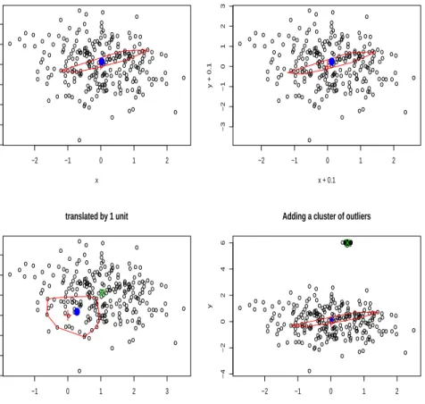
An important remark about anchored estimators is that they are not translation equivariant. A sort of hard shrinkage towardsx0 happens: as soon as a translation
moves X far enough from x0, the translation equivariant solution is mapped in a
bounded set close tox0. This is illustrated in Figure 1, where we setα = 80%. In
the top left panel, the MCD and anchored MCD coincide (blue dot). In the top right panel, data are translated by a small amount and still the anchorx0(red cross) is within
the convex hull of the optimal MCD subset. If we translate by a larger amount, the anchor is now poorly chosen and the MCD (greenX) does not coincide with the an-chored MCD anymore (bottom left panel). A data-dependent choice ofx0, such as the
one adopted in§4, will help to prevent this situation. The fact that anchoring is useful is illustrated in the bottom right panel, where a cluster of outliers is added. The MCD is now within this cluster, as its points have a very small scatter, while the anchored MCD is not affected.
Another important remark concerns the seemingly restrictive assumption that sub-stitution of points inXis restricted to a subset which guarantees existence of a convex hull containingx0. It shall be noted though that the substituted points are (as usual)
replaced by arbitrary points. Additionally, as said before,x0 need not be chosen in
advance and can hence be tuned to guarantee existence. Once the anchored estimators exist, they cannot break down. For this reason, it can be readily shown that the
addi-tion breakdown point – which is based on adding contaminating points to the data set,
instead of replacing them: see Hennig (2004) – is not restricted.
Theorem 1 Fixg >0as the number of points to be trimmed. Suppose that the chosen
anchoring pointx0belongs to the convex hull ofX. Then, the anchored estimator of
location (17) has an addition breakdown point ofg/(n+g).
Proof. Suppose thatg+1contaminated points are added. Since onlygcan be trimmed,
at least one contaminated point will be included in the estimators and possibly lead to break down. Therefore an upper bound for the addition breakdown point isg/(g+n). Note now that, since thenpoints originally included in the dataX are not modified or removed, by assumption onx0the anchored estimator exists with at least one solution
such that
|tx0(X)| ≤T
for a certain finite valueT which depends only on the original data. It only remains to show that the anchored estimatortx0(X)chooses one of the bounded solutions,
which is straightforward as the unbounded solutions either have unbounded objective functions, or anyx0∈Rvdoes not belong to their convex hull.
A fairly similar discussion can be put forward for affine equivariant estimators. Recall for instance that an estimator of locationt(·)is affine equivariant ift(Ax+c) =
At(x) +c. Davies (1987) shows that the BP of any affine equivariant covariance esti-mator is at most given by (8), which might be much smaller than 50%. The trimming level obviously has an upper bound of⌊(n−v−1)⌋/nto guarantee that the estimated covariance matrix is positive definite. If we use a trimming levelα∈(0,1−(v+1)/n), a reasoning along the lines of the proof of Proposition 3 can be used to show that the BP of the anchored estimator of scatter is equal to(⌊nα⌋+ 1)/n.
−2 −1 0 1 2 −4 −3 −2 −1 0 1 2 original x y −2 −1 0 1 2 −3 −2 −1 0 1 2 3 translated by 0.1 units x + 0.1 y + 0.1 −1 0 1 2 3 −3 −2 −1 0 1 2 3 translated by 1 unit x + 1 y + 1 −2 −1 0 1 2 −4 −2 0 2 4 6
Adding a cluster of outliers
x
y
Figure 1: Anchoring estimators in action. The red cross indicates the anchoring point. The blue dot is the anchored estimator, surrounded by the convex hull (containing the anchoring pointx0). When this differs from the MCD, the MCD is shown as a green X.
The anchored estimator of scatter is found along the same lines as the anchored estimator of location: given a sample ofv-variate observationsX ={x1, . . . , xn}and
trimming levelα, the anchored estimators of the location parameterµand scatterΣare
tx0(X) = 1 ⌊n(1−α)⌋ ⌊n(1−α)⌋ X i=1 x‡i, Tx0(X) = ζα ⌊n(1−α)⌋ ⌊n(1−α)⌋ X i=1 (x‡i−tx0(X))(x ‡ i−tx0(X)) ′, (20) wherex‡⌊n(1−α)⌋={x‡1, . . . , x ‡
⌊n(1−α)⌋}is the subset of⌊n(1−α)⌋points ofX
min-imizing the objective function among all subsets whose convex hull containsx0.
Theorem 2 Assume contaminating points are in general position, that is, they do not
lie in a lower dimensional space. For a fixedα, consider the substitution of(⌊nα⌋)
points ofX such that the chosen anchoring pointx0belongs to the convex hull of the
remaining⌈n(1−α)⌉. Forα∈(0,1−(v+ 1)/n), the anchored estimator of scatter
has (restricted) BP(⌊nα⌋+ 1)/n.
Proof. The fact that(⌊nα⌋+ 1)/nis an upper bound is shown as in the proof of
Propo-sition 3. In fact, ifα= 1−(v+ 1)/n, no positive definite solution exists. For smaller values ofα, if we replace(⌊nα⌋+ 1)observations with arbitrary values, at least one of these values would not be discarded. Consequently, all solutions would become un-bounded. To see that(⌊nα⌋+ 1)/nis also a lower bound, we need to show two things. First, we need to show that the minimum covariance determinant cannot be arbitrarily increased. To see this, replace at most⌊nα⌋points ofXwith arbitrary points to obtain Y. Since there are⌊n(1−α)⌋points of the original sampleX, and by assumption there exists at least one anchored solutionΣˆ, there exist at least one solution with bounded determinant. The anchored estimator chooses one of the bounded solutions as the un-bounded solutions either have unun-bounded objective functions, or anyx0∈Rvdoes not
belong to their convex hull. Secondly, we need to show that the minimum covariance determinant cannot be arbitrarily decreased. This is straightforward from the assump-tion thatXand contaminating points are in general position (see detailed reasoning on this point in Davies (1987); Lopuha¨a and Rousseeuw (1991)).
As in Theorem 1, it is possible to show that the addition BP forΣˆ is unrestricted.
4
Wild adaptive trimming for robust cluster analysis
Our main strategy for performing robust cluster analysis through wild (adaptive) trim-ming follows the general principle that several analyses from more than one starting point are necessary to reveal the clustering structure. When the data come from model (10), the trimmed estimators computed withα <0.5typically use observations from several clusters and may thus fail to identify the different populations. On the other hand, starting with a subset of observations belonging to the same population would lead to high values of the robust distances (7) for the observations from other clus-ters, which are then detected as outliers. Empirical evidence of this behaviour has been shown in an exploratory context (see, e.g., Atkinson et al., 2004, 2017), while the robustness properties of§3 provide a more general theoretical justification.
With a slight abuse of notation, in what follows we letG0(x)denote the distribution
function of one of the normal mixture components in (10), to be taken as the target population with parametersµandΣ, instead of the distribution of the whole mixture. That is, we now let
G0(x) = Φµ,Σ(x)
as in (2), with
µ=µk∗, Σ = Σk∗
for a givenk∗∈ {1, . . . , K}. Correspondingly, we takeG
1(x)to be the (unspecified)
distribution function mixturing all the other components and the contaminated obser-vations. It is then crucial to use trimming levels in the computation of (3) and (4) that could lead to estimation ofµandΣ, and thus to identification ofG0(x), under model
(1). This task is clearly made possible by the adoption of a wild trimming approach, and by the fact that, as noted,G0(x)now identifies a single population.
We suggest a divisive clustering approach that splits theK-population estimation problem defined by (10) intoK one-population steps, which take advantage of the good breakdown properties of wild trimming estimators and do not force all units to be classified. In an adaptive framework, we start the trimming procedure from values ofαmuch larger than 0.5, typically including onlyv+ 1 observations or a slightly larger number, in the first estimation step. The details of our robust divisive clustering procedure are described below. For concreteness we refer to wild adaptive trimming through the FS, but any other procedure that shares the same properties (e.g., based on the MCD) could be potentially used.
1. Computation of minimum Mahalanobis distances from random starts. We performRforward searches starting fromRrandom subsets of sizem0=v+ 1.
For all the searches and each ml = ⌊(1−αl)n⌋, l = 0, . . . , L, we control the ratio between the maximum and the minimum eigenvalue of the estimated covariance matrix. We impose that this ratio is smaller than a certain threshold, sayc, in order to avoid the detection of spurious groups due to the presence of almost collinear points. We discard the searches (whose number, say, isr) for which this condition is not fulfilled. For each of theR−rremaining searches and each subset sizeml, we store the value of the minimum Mahalanobis distance of the units not belonging to the fitting subset:
dmin(ml) = minqd2
i,αl, i /∈ι
†
αl, (21) where, forl = 0, . . . , L,d2
i,αl is defined as in (16). In all the examples that follow we setR= 500, although a larger number of random searches should be performed in the case of big data sets. Indeed, it usually suffices that the majority of points of the starting subset belong toG0(x)in order to obtain high values of
the robust distances (7), and thus of (21), for the observations not belonging to this population. The probability of randomly selectingη0 = ⌊m0/2⌋+ 1
observations from a sample ofN units drawn fromG0(x)is ηN0/ ηn0, which
is often not exceedingly small whenm0=v+ 1andnis of the order of just a
to recover from a bad starting point, by replacing contaminated observations in the fitting subset with others coming fromG0(x)(see, e.g., Atkinson et al.,
2004). This phenomenon, which is called “interchange”, clearly enhances the diagnostic power of (21) and increments the probability of detectingG0(x)with
a fixed number of random starts, as our empirical examples show in§5. 2. Envelope calibration. If all the units inι†
αl come fromG0(x)and the units not inι†
αlcome from different populations (separated fromG0(x)), the observation giving rise todmin(ml)will be an outlier and its distance will be large if com-pared to the distances of the units in ι†αl. We thus need to compare the value ofdmin(ml)with the quantiles of its distribution for each stepl = 0, . . . , L. The simulation results given in Atkinson et al. (2006) show that the envelopes ofdmin(ml)starting from random subsamples are much larger than those based on robust initialization whenml< n/3, especially in the case of extreme quan-tiles. However, this difference decreases aslincreases and becomes negligible for subsets of sizeml > n/2. A reliable approximation to envelopes based on the theory of order statistics is given in Riani et al. (2009), but only for the case of robust initialization.
Since we are interested in values ofmlwhich may be much smaller thann/2, we have simulated the 1%, 50%, 75%, 90%, 95%, 99%, 99.9%, 99.99%, 99.999% and 99.9999% percentiles of dmin(ml), for l = 0, . . . , L, under the normal modelG0(x) = Φµ,Σ(x)and using 1,000,000 random initializations. In what
follows we call these envelopes the null envelopes, since they correspond to the situation where only one population exists, i.e. (10) holds withK = 1. They have been obtained for each value ofv≤10and a grid of values ofnfrom 50 to 2000. Ifnis not in the grid we use linear interpolation between the two adjacent values.
3. Convex hull constraint and pruning. The observations entering in the first steps of the FS are those more likely to come fromG0(x). It is thus natural to
adopt a data-dependent anchoring procedure and to fix the anchorx0as a point
which lies inside the convex hull of the observations belonging to the fitting subset ι†
αl. In this way the anchor will not be too far from the true mode of
G0(x), at least whenG0(x)belongs to the elliptical family, untilι†αlremains free of contaminated observations. Therefore, we findαlas the trimming level prior to the first exceedance of the null envelope ofdmin(ml)for a certain probability level, sayς. As we see in§5, in the first steps just after the random start the values ofdmin(ml)may be above the 99% threshold due to random fluctuations and the number of different trajectories diminishes considerably asmlincreases. In fact, all random starts of sizem0=v+ 1initialized with more than⌊v/2⌋+ 1
observations fromG0(x), as soon as the subset size grows, tend to remove the
observations from the other groups and include other observations fromG0(x).
Therefore, after a few steps, theR−rsearches naturally anchor themselves to a few centroids and a few covariance matrices. In what follows we callm† the
subset size for which we start to impose the “anchoring”. More precisely,
wheredς(ml)is theς-quantile ofdmin(ml)andmingrsizeis the minimum group size that we are willing to tolerate. For allR−rtrajectories we monitor whether the units which are progressively included forml> m†satisfy the
con-vex hull constraint (18). Therefore in practice there is no need to choose a partic-ular anchoring point, such as the centroid or the median of the units belonging to subset at stepm†, because the satisfaction of the convex hull constraint ensures
we anchor so to obtain an estimator which cannot break down (see Proposition 3). As a result of this procedure we prune some of the trajectories ofdmin(ml), i.e. their monitoring ends much earlier than at the final stepl =Lbecause the convex hull constraint fails to be satisfied. Letm†+atbe the final subset size
for trajectoryt(t = 1, . . . , R−r). In the examples which follow, in order to obtain a satisfactory degree of pruning, we takeς = 0.9999. It shall be noted that identical results can be obtained if we increase the confidence band to 99.9999%, or decrease it to 99%. In the latter case, however, the number of random starts which must be used has to be considerably increased. Otherwise, we may lose trajectories which completely end up into one group but which, due to random fluctuations, are pruned before the peak due to loss of anchorage because the convex hull is too “small”.
4. Extreme exceedance of null envelopes. The envelopes ofdmin(ml)are point-wise because their confidence level is referred to a fixed subset sizeml. In the adaptive trimming framework of the FS we potentially make many comparisons, one for each value ofml. Our detection rule thus needs to allow for simultaneity. In order to avoid random exceedances, we select all the prunedR−rtrajectories ofdmin(ml)for which there is an exceedance of a very extreme threshold of the null envelope, saydς∗(ml). Letd(t)
min(ml)be the trajectory for thet-th pruned
search. Then,m∗
t is the first subset size for which
d(mint) (ml)> dς∗(ml) ml=m†, m†+1, ..., m†+at, t= 1,2, . . . , N−r.
(22) In what follows we takeς∗= 0.999999.
5. Divisive split. Given that our purpose is to identify and remove first the group which is most remote from the others, among the searches for which condition (22) is verified we take the one (say thet∗) for which
rsj∗ = arg max t rst, (23) where rst= max ml d(mint) (ml)−d0.5(ml) d0.99(ml)−d0.5(ml). (24) We then assign theml−1observations which formι†
αl−1to a tentative group.
6. Iteration of previous steps. The previous steps (1-5) are iterated until with the units which are left out we end up with one of the two following cases: A) their number is smaller thanmingrsize. B) we do not observe any exceedance of the extreme null envelope.
7. Robust tree. At the end of the procedure we display the binary splits and the resulting clusters by a tree-like structure. In the vertical axis of the tree we show the distance levelrsj∗ (see Equation 23) in which the various groups are
formed (it is also possible to use a rescaled version ofrsj∗ in case one wants
to standardize the results over different datasets). One additional bonus of the suggested procedure is that it enables us to immediately appreciate the degree of separation (overlapping) of each group with the remaining part of the sample. Clearly the higher is the value of internal cohesion of a group with respect to the rest, the greater is the value ofrsj∗. The outliers and the other units not assigned
to any of the tentative groups are left aside, thus making the tree robust. We note that, by considering a crude rule like (22), we are likely not to consider all units belonging to a particular group. Therefore, a successive reweighting step (which in the spirit of the FS can be performed adaptively; see also Dotto et al. (2017)) is necessary for refining the tentative groups which have been found. A preliminary proposal, rooted in an exploratory framework, is described in (Atkinson et al., 2004, p. 369). However, in our divisive procedure, the fact of leaving out the units which are at the boundary of a particular group helps to detect the remaining groups in the successive steps of the procedure. The null envelopes obtained after removal of the first cluster, being based on a number of observations larger than the number of units belonging to the remaining populations, will be flatter and tighter, thus increasing the probability of exceedance of the extreme envelope in the central part of the algorithm.
5
Robust divisive clustering in action
5.1
Geyser data
In order to illustrate the performance of our divisive clustering procedure, we start by considering the “geyser data set”, a well known application in robust clustering (see, e.g., Garc´ıa-Escudero and Gordaliza, 1999). This bivariate data set, obtained from the Old Faithful Geyser, contains the eruption length and the length of the previous eruption for 271 eruptions of this geyser. Both variables are measured in minutes. The data show the presence of three main groups. Close to the origin there is also a small group of “short followed by short” eruptions, which are not very common (6 observations, i.e. 2.2% of the sample size).
The left panel of Figure 2 shows the forward plot of the trajectories of minimum Mahalanobis distances computed from 500 random starts, together with 1%, 50%, 99% and 99.9999% simulation envelopes from model (10) withK= 1. To provide a com-parison with previous applications of the FS, in this plot we do not anchor the estimator and all trajectories are monitored up toml=n. In presence of a homogenous popula-tion of sizen, all theRtrajectories ofdmin(ml)rapidly converge to a single trajectory which tends to remain inside the envelopes up toml =n. In this situation the shape of the envelopes ofdmin(ml)looks like the prows of viking longships, i.e. they are virtually horizontal in the centre of the plot and rapidly increase asmltends tondue to the inclusion in the final steps of the observations coming from the tails of the dis-tribution. On the contrary, if model (10) holds withK >1and if there is a group with
size (say)n×0.2, for all the searches which start in this group we observe a rapid increase in the trajectory ofdmin(ml)asmltends ton×0.2. The same also typically happens for the searches such that them0=v+ 1initial observations contain at least
⌊v/2⌋+ 1units from the group, due to the interchange of units from other groups as the subset size grows. After this subset size, as observations from other groups joinι†
αl, we are likely to observe a sudden decrease in the trajectory ofdmin(ml)and its values will be even below the lower quantiles of the null envelopes for a single homogenous population of sizen. It is an evidence of the extreme effect that contamination by dif-ferent populations can produce on parameter estimates. The same effect will lead to a “loss of anchorage” when we impose the convex hull constraint (18). The plot in the left panel of Figure 2 reveals some trajectories which go persistently above the extreme 99.9999% threshold around subset sizeml= 90. Similarly, aroundml = 170we can observe two trajectories which go outside the extreme envelope and, to a minor extent, another trajectory which spends some time above this threshold just beforeml= 200. All trajectories converge into one fromml = 230onwards. It is interesting to notice that before all the trajectories converge into one there is a persistent exceedance of the lower threshold. The same phenomenon is also visible aroundml= 100, shortly after the first peak. In this example, given that the first exceedance of the extreme envelope is whenm† = 76, for each ofR−rtrajectories we impose the convex hull constraint
from this step and findm† +at(t = 1,2, . . . , R−r). The right panel of Figure 2
shows the pruned trajectories. For example, for the 3 trajectories exceeding the ex-treme envelope the constraint is fulfilled up tom†+a
1 = 107,m†+a2 = 107and
m†+a
3= 97. In order to understand which is the group which is most remote from
the others we compute indexrstgiven in equation (24), select the trajectory associated with the maximum value and select the step where first exceedance of extreme enve-lope takes place. In this case this leads to the identification of a first tentative group made up ofm∗= 83units with a corresponding value ofrsj∗ = 9.71
It is interesting to notice that the number of searches which end up with the three trajectories is 152, 144 and 177, respectively. Therefore, starting from 500 random ini-tializations in almost 95% of the times we have reached trajectories which collapse into just one group. This also implies that in this example it was not necessary to consider as many as 500 random starts to elucidate the existence of three distinct groups.
The random start FS procedure is repeated using the remaining 188 units, after removal of tentative Group 1. The left panel of Figure 3 shows the new pruned trajec-tories ofdmin(ml)with the corresponding null envelopes based onn= 188. The same argument described above leads to the identification of a second tentative group, again of size 83 with a corresponding value ofrsj∗ = 9.23. The results of the third iteration
of our procedure are displayed in the right panel of Figure 3, obtained after removal also of tentative Group 2. The pruned trajectories ofdmin(ml), with null envelopes based onn = 105units, now lead to the identification of a third tentative group of size 84 withrsj∗ = 4.56. These three steps leave us with 21 unassigned units without
apparent structure. Therefore, the procedure terminates and we setK= 3.
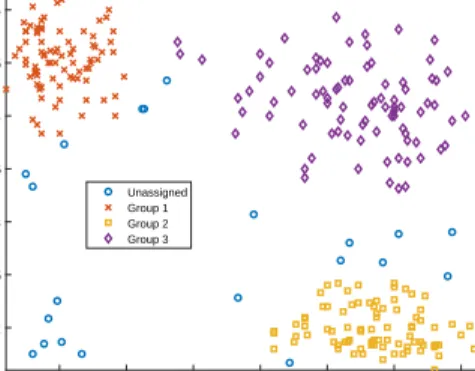
The binary splits and the resulting clusters are displayed in a tree-like structure in Figure 4, while our robust tentative clustering of these data is given in Figure 5. The latter plot, given that it has on the vertical axis the value ofrsj∗, not only shows
50 100 150 200 250 2 3 4 5 20 40 60 80 100 2 3 4 5
subset size
m
lsubset size
m
lFigure 2: Geyser data. Left panel: forward plot trajectories of minimum Mahalanobis distances from 500 random starts monitored up toml =nwith 1%, 50%, 99% and extreme 99.9999% null envelopes. Right panel: trajectories of minimum Mahalanobis distances pruned after anchoring the estimators and imposing the convex hull con-straint. In the right panel the horizontal axis goes up to110≈max(m†+at) = 107).
Indeed, the group on the top left of Figure 5 (which is found in the first divisive step) appears to be the most compact one, while the cluster on the top right (which is found in the third divisive step) is the most dispersed one. The units not assigned to any of the three main clusters correspond to some borderline observations and to the peculiar set of “short followed by short” eruptions. We do not insist in labelling these eruptions as outliers, or as representatives of a fourth, more uncommon, population. We believe that the final interpretation will strongly depend on subject-matter knowledge and on the purposes of the study. The important statistical finding from our robust cluster analysis is that they do not belong to the three main populations that our method identifies.
5.2
M5 data
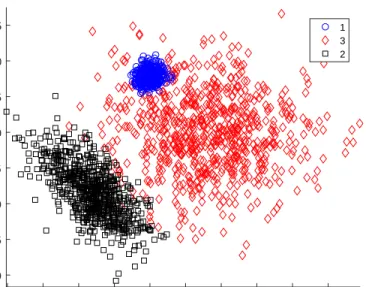
The geyser data set originates from well separated populations, with the possible addi-tion of markedly different outliers. Another applicaaddi-tion with similar features (to Swiss banknotes) is described in the Supplementary Material. We now show the performance of our divisive procedure in a case with highly overlapping populations. The M5 data were introduced by Garc´ıa-Escudero et al. (2008) for assessing some trimming-based robust clustering methods. The data (shown in Figure 6) are obtained from three nor-mal bivariate distributions with fixed centers but different scales and proportions. One of the components strongly overlaps with another one. To these data a uniform noise contamination is sometimes added. However, in this application we concentrate on the “uncontaminated version” of the data set withn= 1800, since our main interest is not on the effect of widespread noise.
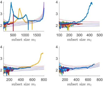
The top left panel of Figure 7 shows the monitoring of the trajectories of mini-mum Mahalanobis distances from 500 random starts without pruning. This plot
dis-20 40 60 80 100 2 3 4 5 20 40 60 80 100 2 3 4 5
subset size
m
lsubset size
m
lFigure 3: Geyser data. Left panel: forward plot of pruned trajectories of minimum Mahalanobis distances after removing the units from the first tentative group. Right panel: forward plot of pruned trajectories of minimum Mahalanobis distances after removing the units from tentative Groups 1 and 2.
plays three distinct trajectories aroundml = 400. It is interesting to see that around
ml = 500 there is a dip below the lower envelope for one trajectory before being absorbed by another one which stands above the upper envelope. This data set has also been analyzed by Atkinson et al. (2015), who manually choose a particular step in the random start procedure and compare the units inside the fitting subset for the various trajectories. The top right panel of Figure 7, which shows the pruned trajecto-ries of the same minimum Mahalanobis distances, avoids this manual choice because it enables us to appreciate that there is only one trajectory which exceeds the extreme threshold and which terminates whenml = 427. All the other trajectories are pruned much earlier and are completely inside the null envelopes. This is an indication that the remaining trajectories refer to searches which include observations from other groups which are outside the convex hull of the reference group and therefore we lose the good propoerties of the anchored estimator. Considering the first exceedance of the extreme envelope leads to the identification of a first tentative group of 308 observations. The two bottom panels show the pruned trajectories of minimum Mahalanobis distances, again from 500 random initializations, in the two successive steps of the divisive pro-cedure. Also in this case pruning enables to identify just one trajectory outside the extreme envelope and leads in a natural way to the identification of the underlying group. The divisive procedure is detailed in Figure 8, while the left panel of Figure 9 shows the scatter plot of the original data with theK = 3tentative groups which have been found and the unclassified units. For clarity of interpretation, in Figure 9 the 99% confidence ellipses have been added using the centroids and the covariance matrices of the estimated groups. The overall performance of our method is very good, with only 3.6% of the assigned observations clustered in the wrong group.
10 9 8 7 6 5 4 3 2 1 0 D is t a n c e le v e l r sj ∗ n=271 Group 1 n1=83 n=188 Group 2 n2=83 n=105 Group 3 n3=84 n=21
Figure 4: Geyser data. Robust tree showing the details of the divisive procedure. The 21 unassigned units clearly stand apart in the last split.
5.3
Comparison with TCLUST
We conclude our empirical analysis by comparing the results of our divisive proce-dure with those obtained through the TCLUST methodology of Garc´ıa-Escudero et al. (2008), Fritz et al. (2012) and Ruwet et al. (2013). TCLUST is a robust model-based clustering technique that relies on constrained maximization of a trimmed version of a generalized classification likelihood function. The constraint is that
maxK k=1˜λ1,k
minKk=1λv,k˜
≤c, (25)
where˜λ1,kandλv,k˜ denote the largest and the smallest eigenvalue ofΣ˜k, respectively,
andc ≥ 1 is a fixed constant specified by the user. Values ofc close to 1 favour solutions with spherical clusters, while high values ofctend to produce one (or more) large and dispersed cluster possibly overlapping with the other groups.
It is important to emphasize that, unlike our method, TCLUST requires to spec-ify in advance a number of important parameters: the number of groupsK, the level of trimmingαto be used in the generalized classification likelihood function and the eigenvalue ratio restriction (25). Our adaptive-trimming divisive procedure finds in-stead suitable values ofK andαfrom the data, while (25) is not needed because we just fit one population at a time. Therefore, we can see this comparison as a worst-case scenario for our technique, since we are not taking advantage of the prior information which is used to initialize TCLUST.
In order to apply TCLUST to the data sets considered in this paper, we use the number of clusters which we have found in an automatic way and we setαequal to
2 2.5 3 3.5 4 4.5 5 Eruption length 2 2.5 3 3.5 4 4.5 5
Previous eruption length
Unassigned Group 1 Group 2 Group 3
Figure 5: Geyser data. Robust tentative clustering intoK = 3main groups after the divisive procedure.
the proportion of units which are left unclassified by our procedure. We also fix the restriction factorc = 100in order to be able to find elongated clusters, such as the one present in the M5 data set. For the geyser data and for the Swiss banknotes (an-alyzed in the Supplementary Material), the results from TCLUST are similar to those obtained with our method. Indeed, the adjusted Rand index between the two cluster-ings is 0.95 for the geyser data and 0.88 for the Swiss banknote data. This means that the performance of our divisive procedure is virtually equivalent to that of TCLUST, provided that the latter is properly tuned through appropriate a priori information. The outcome is somewhat different in the case of the M5 data set, for which the right panel of Figure 9 shows the three-group robust clustering obtained by TCLUST. Although the overall performance of this clustering is very good (the misclassification rate is 2.4%), it is clear that TCLUST underestimates the size of Population 3. The key issue for explaining such a poorer performance in the identification of a dispersed group is the rigid use of the trimming levelαmade by TCLUST. Since in this example there are no outliers, fixingα≫0leads TCLUST to trim all the observations that lie at the bor-der of the more dispersed population, which is not instead the case for our procedure. Through our adaptive trimming approach, we are able to detect the population bor-ders in a flexible way and without penalizing uncommon structures too much. On the contrary, TCLUST treats the farthest observations from Population 3, and in particular those lying above Population 1, as uniform noise to be trimmed. We may thus expect an improvement in the performance of TCLUST if the method could be embedded in an adaptive trimming framework similar to that considered in our work.
6
Concluding remarks
This work is motivated by the requirement of robust and efficient procedures for clus-tering multivariate data generated by mixture model (10) with additional contamina-tion. Our approach replaces the originalK-population (robust) estimation problem withKdistinct (robust) one-population steps, which take advantage of the good
break--20 -15 -10 -5 0 5 10 15 20 25 -20 -15 -10 -5 0 5 10 15 1 3 2
Figure 6: M5 data. Scatter plot of the two variables. Cluster 1 is very tight and lies completely inside cluster 2. Clusters 2 and 3 also overlap.
down properties of trimmed estimators. For this purpose, we have studied the theoreti-cal behaviour of trimmed estimators when the trimming level exceeds the usual bound of 0.5, thus relaxing the familiar condition that at least half of the data should corre-spond to the main population. We have shown that exact affine equivariance must be lost, but it is a reasonable price to be paid in order to achieve arbitrarily high breakdown for the resulting trimmed estimators. This conclusion parallels similar findings in other situations where contamination produces only a minority of “good” observations, as in the case of cell-wise contamination (see, e.g., Farcomeni, 2014a,b; Agostinelli et al., 2015; Rousseeuw and Van den Bossche, 2017). We also support the use of adaptive trimming schemes, in order to explore the effect of different levels of trimming and to find a sensible trade-off between robustness and efficiency. A further bonus of our methodology is its ability to provide a reliable choice of the usually unknown number of groups that correspond to genuine populations in model (10).
We have provided empirical evidence that our technique can perform well even when there is considerable overlap among the groups. The price that we pay for sep-arating the groups when they partially overlap is to trim a bit more than necessary in steps (d) and (e) of our divisive procedure. Even if our trimming approach is adaptive and provides a good trade-off between robustness and efficiency, there is the need of additional theoretical work in order to find a stopping rule that guarantees the required simultaneous test size when testing for exceedances of null envelopes. Similarly, pre-cise estimation of the contamination rate in (1) and of the mixing proportions in (10) are still open issues. A refined estimate of the population sizes, as well as a refined identification of group membership, could be obtained by adding a confirmatory step to the tentative clustering that we obtain by our divisive procedure. The confirmatory
Figure 7: M5 data. Top left panel: trajectories of minimum Mahalanobis distances from 500 random starts without pruning, together with 1%, 50%, 99% and 99.9999% envelopes. Top right panel: forward plot of the same pruned trajectories. Bottom left panel: forward plot of pruned trajectories of minimum Mahalanobis distances after removing the units from the first tentative group. Bottom right panel: forward plot of pruned trajectories of minimum Mahalanobis distances after removing the units from the first two tentative groups.
20 18 16 14 12 10 8 6 4 2 0 D is t a n c e le v e l r sj ∗ n=1800 Group 1 n1=308 n=1492 Group 2 n2=569 n=923 Group 3 n3=683 n=240
Figure 8: M5 data. Robust tree showing the details of the divisive procedure.
-20 -10 0 10 20 30 -20 -10 0 10 -20 -10 0 10 20 30 -20 -10 0 10 3 2 1 0
Figure 9: M5 data. Left panel: tentative clustering from the divisive procedure. Right panel: tentative clustering from TCLUST whenKis set equal to 3 and the same trim-ming level is used as in the divisive procedure. In both panels 99% confidence el-lipses have been added using the centroids and the covariance matrices of the estimated groups.
step could also help to separate small and concentrated groups of contaminated obser-vations from background noise (Hennig and Liao, 2013; Coretto and Hennig, 2016), as well as to highlight the relationship between our procedure and robust fitting of mixture models. Both these topics are the subject of ongoing research.
Acknowledgements
The authors are grateful to the Editor, an Associate Editor and three anonymous ref-erees for very detailed and thoughtful suggestions. They also thank Gunter Ritter for discussion on a previous draft.
This research benefits from the HPC (High Performance Computing) facility of the University of Parma, Italy
MR gratefully acknowledges support from the CRoNoS project, reference CRoNoS COST Action IC1408.
References
Agostinelli, C., A. Leung, V. J. Yohay, and R. H. Zamar (2015). Robust estimation of multivariate location and scatter in the presence of cellwise and casewise contami-nation. Test 24, 441–461.
Atkinson, A. C., A. Cerioli, G. Morelli, and M. Riani (2015). Finding the number of disparate clusters with background contamination. In B. Lausen, S. Krolak-Schwerdt, and M. B¨ohmer (Eds.), Data Science, Learning by Latent Structures, and
Knowledge Discovery, pp. 29–42. Heidelberg: Springer-Verlag.
Atkinson, A. C., M. Riani, and A. Cerioli (2004). Exploring Multivariate Data with
the Forward Search. New York: Springer–Verlag.
Atkinson, A. C., M. Riani, and A. Cerioli (2006). Random start forward searches with envelopes for detecting clusters in multivariate data. In S. Zani, A. Cerioli, M. Riani, and M. Vichi (Eds.), Data Analysis, Classification and the Forward Search, pp. 163– 171. Berlin: Springer-Verlag.
Atkinson, A. C., M. Riani, and A. Cerioli (2017). Cluster detection and clus-tering with random start forward searches. Journal of Applied Statistics,
DOI:10.1080/02664763.2017.1310806.
Butler, R. W., P. L. Davies, and M. Jhun (1993). Asymptotics for the minimum covari-ance determinant estimator. The Annals of Statistics 21, 1385–1400.
Cator, E. A. and H. P. Lopuha¨a (2012). Central limit theorem and influence function for the MCD estimators at general multivariate distributions. Bernoulli 18, 520–551. Cerioli, A. (2010). Multivariate outlier detection with high-breakdown estimators.
Cerioli, A., A. Farcomeni, and M. Riani (2013). Robust distances for outlier-free goodness-of-fit testing. Computational Statistics and Data Analysis 65, 29–45. Cerioli, A., A. Farcomeni, and M. Riani (2014). Strong consistency and robustness of
the forward search estimator of multivariate location and scatter. Journal of
Multi-variate Analysis 126, 167–183.
Cerioli, A., M. Riani, A. C. Atkinson, and A. Corbellini (2017). The power of mon-itoring: how to make the most of a contaminated multivariate sample. Statistical
Methods and Applications, DOI: 10.1007/s10260–017–0409–8.
Clarke, B. and D. Schubert (2006). An adaptive trimmed likelihood algorithm for identification of multivariate outliers. Australian and New Zealand Journal of
Statis-tics 48, 353–371.
Coretto, P. and C. Hennig (2016). Robust improper maximum likelihood: tuning, computation, and a comparison with other methods for robust Gaussian clustering.
Journal of the American Statistical Association 111, 1648–1659.
Cuesta-Albertos, J. A., C. Matr´an, and A. Mayo-Iscar (2008). Trimming and likeli-hood: Robust location and dispersion estimation in the elliptical model. The Annals
of Statistics 36, 2284–2318.
Davies, P. L. (1987). Asymptotic behaviour of S-estimates of multivariate location parameters and dispersion matrices ellipsoid estimator. The Annals of Statistics 15, 1269–1292.
Dotto, F., A. Farcomeni, L. A. Garc´ıa-Escudero, and A. Mayo-Iscar (2017). A reweighting approach to robust clustering. Statistics and Computing in press,
https://doi.org/10.1007/s11222–017–9742–x.
Farcomeni, A. (2014a). Robust constrained clustering in presence of entry-wise out-liers. Technometrics 56, 102–111.
Farcomeni, A. (2014b). Snipping for robust k-means clustering under component-wise contamination. Statistics and Computing 24, 907–919.
Farcomeni, A. and L. Greco (2015). Robust Methods for Data Reduction. Boca Raton: Chapman and Hall/CRC.
Fritz, H., L. A. Garc´ıa-Escudero, and A. Mayo-Iscar (2012). tclust: An R package for a trimming approach to Cluster Analysis. Journal of Statistical Software 47, https://www.jstatsoft.org/v47/i12.
Garc´ıa-Escudero, L. A. and A. Gordaliza (1999). Robustness properties ofkmeans and trimmedkmeans. Journal of the American Statistical Association 94, 956–969. Garc´ıa-Escudero, L. A., A. Gordaliza, C. Matr´an, and A. Mayo-Iscar (2008). A general trimming approach to robust cluster analysis. The Annals of Statistics 36, 1324– 1345.
Hardin, J. and D. M. Rocke (2005). The distribution of robust distances. Journal of
Computational and Graphical Statistics 14, 910–927.
Hennig, C. (2004). Brekdown points for maximum likelihood estimators of location-scale mixtures. Annals of Statistics 32, 1313–1340.
Hennig, C. and T. Liao (2013). How to find an appropriate clustering for mixed-type variables with application to socio-economic stratification. Applied Statistics 62, 309–369.
Huber, P. J. and E. M. Ronchetti (2009). Robust Statistics. Second Edition. Hoboken: Wiley.
Hubert, M., P. J. Rousseeuw, and S. Van Aelst (2008). High-breakdown robust multi-variate methods. Statistical Science 23, 92–119.
Johansen, S. and B. Nielsen (2016a). Analysis of the Forward Search using some new results for martingales and empirical processes. Bernoulli 22, 1131–1183.
Johansen, S. and B. Nielsen (2016b). Asymptotic theory of outlier detection algorithms for linear time series regression models (with discussion). Scandinavian Journal of
Statistics 43, 321–348.
Lopuha¨a, H. P. and P. J. Rousseeuw (1991). Breakdown points of affine equivariant estimators of multivariate location and covariance matrices. The Annals of
Statis-tics 19, 229–248.
Riani, M., A. C. Atkinson, and A. Cerioli (2009). Finding an unknown number of multivariate outliers. Journal of the Royal Statistical Society, Series B 71, 447–466. Riani, M., A. Cerioli, A. C. Atkinson, and D. Perrotta (2014). Monitoring robust
regression. Electronic Journal of Statistics 8, 646–677.
Ritter, G. (2014). Robust Cluster Analysis and Variable Selection. Boca Raton: Chap-man and Hall/CRC.
Rousseeuw, P. J. and A. M. Leroy (1987). Robust Regression and Outlier Detection. New York: Wiley.
Rousseeuw, P. J. and W. Van den Bossche (2017). Detecting deviating data cells.
Tech-nometrics, DOI: 10.1080/00401706.2017.1340909.
Ruwet, C., L. A. Garc´ıa-Escudero, A. Gordaliza, and A. Mayo-Iscar (2013). On the breakdown behavior of the TCLUST clustering procedure. Test 22, 466–487.