Efficient estimation of Markov regime-switching models: An application to electricity spot prices

(1)

HSC/11/02

HSC Research Rep

ort

Efficient estimation of

Markov

regime-switching models: An

application to electricity

spot prices

Joanna Janczura*

Rafał Weron**

* Hugo Steinhaus Center, Wrocław University of

Technology, Poland

** Institute of Organization and Management, Wrocław

University of Technology, Poland

Hugo Steinhaus Center

Wrocław University of Technology

Wyb. Wyspiańskiego 27, 50-370 Wrocław, Poland

http://www.im.pwr.wroc.pl/~hugo/

(2)

(will be inserted by the editor)

Efficient estimation of Markov regime-switching models:

An application to electricity spot prices

Joanna Janczura · Rafa l Weron

Received: September 29, 2011

Abstract In this paper we discuss the calibration of models built on mean-reverting processes combined with Markov regime-switching (MRS). We pro-pose a method that greatly reduces the computational burden induced by the introduction of independent regimes and perform a simulation study to test its efficiency. Our method allows for a 100 to over 1000 times faster calibra-tion than in case of a competing approach utilizing probabilities of the last 10 observations. It is also more general and admits any value ofγ in the base regime dynamics. Since the motivation for this research comes from a recent stream of literature in energy economics, we apply the new method to sample series of electricity spot prices from the German EEX and Australian NSW markets. The proposed MRS models fit these datasets well and replicate the major stylized facts of electricity spot price dynamics.

Keywords Markov regime-switching· energy economics · electricity spot price·EM algorithm·independent regimes

1 Introduction

The underlying idea behind Markov regime-switching (MRS; or hidden Markov models – HMM) is to represent the observed stochastic behavior of a specific time series by two (or more) separate states or regimes with different un-derlying stochastic processes. The switching mechanism between the states is

Joanna Janczura

Hugo Steinhaus Center for Stochastic Methods, Wroc law University of Technology, Wyb. Wyspia´nskiego 27, 50-370 Wroc law, Poland

E-mail: [email protected] Rafa l Weron

Institute of Organization and Management, Wroc law University of Technology, Wyb. Wyspia´nskiego 27, 50-370 Wroc law, Poland

(3)

Nov 22, 2007 Dec 22, 2007 Jan 21, 2008 0 50 100 150 Days

EEX price [EUR/MWh]

Base Spike Drop

May 16, 2007 Jun 15, 2007 Jul 15, 2007 2.5 3 3.5 4 4.5 5 5.5 Days NSW log−price [AUD/MWh] Base Spike

Fig. 1 Deseasonalized mean daily electricity spot prices from the European Energy Ex-change (EEX, Germany; left) and the New South Wales Electricity Market (NSW, Aus-tralia;right). Note, that the right panel uses a logarithmic scale to dampen the extreme spikiness of the Australian NSW prices, which can reach up to 10000 AUD/MWh during peak hours. The changes of dynamics (regime switches) are clearly visible in both cases. The prices classiﬁed as spikes or drops are denoted by dots or ‘x’ (see Section 5 for model details).

assumed to be an unobserved (latent) Markov chain. Such models have at-tracted a lot of attention in the recent years, not only in econometrics but also in other as diverse fields of science as population dynamics, speech recog-nition, river flow analysis or traffic modeling (Fink, 2008; Hahn et al., 2009; Hamilton, 2008; Luo and Mao, 2007). This paper is motivated by yet another stream of literature – electricity spot price models in energy economics (Bier-brauer et al., 2007; De Jong, 2006; Erlwein et al., 2010; Huisman and Mahieu, 2003; Janczura and Weron, 2010; Kanamura and ¯Ohashi, 2008; Karakatsani and Bunn, 2008; Kholodnyi, 2005; Mari, 2008; Mount et al., 2006; Weron, 2009). MRS models have seen extensive use in this area due to their relative parsimony and the ability to capture the unique characteristics of electricity spot prices.

Recall, that electricity cannot be stored economically and requires imme-diate delivery. At the same time end-user demand shows high variability and strong weather and business cycle dependence. Effects like power plant out-ages, transmission grid (un)reliability and strategic bidding add complexity and randomness. The resulting spot prices exhibit strong seasonality on the annual, weekly and daily level, as well as, mean reversion, very high volatility and abrupt, short-lived and generally unanticipated extreme price spikes or drops (Benth et al., 2008; Eydeland and Wolyniec, 2003; Weron, 2006). What is more, these spikes tend to cluster. Like in Figure 1 where two sample spot price trajectories are plotted (for more evidence and discussions see Chris-tensen et al., 2009; Janczura and Weron, 2010). The latter feature renders the very popular class of jump-diffusion models impractical, as they cannot exhibit consecutive spikes with the frequency observed in market data.

In contrast, MRS models allow for consecutive spikes in a very natural way. Also the return of prices after a spike to the ‘normal’ regime is straightforward,

(4)

as the regime-switching mechanism admits temporal changes of model dy-namics. MRS models are also more versatile than the popular hidden Markov models (HMM; in the strict sense, see Cappe et al., 2005), since they allow for temporary dependence within the regimes, in particular, for mean reversion. As the latter is a characteristic feature of electricity prices it is important to have a model that captures this phenomenon. Indeed, the base regime is typically modeled by a mean-reverting diffusion (Huisman, 2009), sometimes heteroskedastic (Janczura and Weron, 2010). For the spike regime(s), on the other hand, a number of specifications have been suggested in the literature, ranging from mean-reverting diffusions to heavy tailed random variables.

Having selected the model class (i.e. MRS), the type of dependence between the regimes has to be defined. Dependent regimes with the same random noise process in all regimes (but different parameters; an approach dating back to the seminal work of Hamilton, 1989) lead to computationally simpler models. On the other hand, independent regimes allow for a greater flexibility and admit qualitatively different dynamics in each regime. They seem to be a more natural choice for electricity spot price processes, which can exhibit a moderately volatile behavior in the base regime and a very volatile one in the spike regime, see Figure 1 (note, that the right panel uses a logarithmic scale to dampen the extreme spikiness of the Australian NSW prices).

Once the electricity spot price model is fully specified we are left with the problem of calibrating it to market data. This challenging process is the focus of this paper. Due to the unobservable switching mechanism, estimation of MRS models requires inferring model parameters and state process values at the same time. The situation becomes more complicated when the individual regimes are independent from each other and at least one of them is mean-reverting. Then the temporal latency of the dynamics in the regimes has to be taken into account.

In this paper we propose a method that greatly reduces the computational burden induced by the introduction of independent regimes in MRS models. Instead of storing conditional probabilities for each of the possible state process paths, our method requires conditional probabilities for only one time-step. Since MRS models can be considered as generalizations of HMMs (Cappe et al., 2005), this result can have far-reaching implications for many problems where HMMs have been applied (see e.g. Mamon and Elliott, 2007).

The paper is structured as follows. In Section 2 we define the MRS models used in this paper. Next, in Section 3 we describe the estimation procedure for parameter-switching models and introduce an approximation to avoid the computational burden in case of independent regimes. In Section 4 a simulation study to test the performance of the proposed method is summarized. Then, in Section 5 an application of the proposed approach to models of wholesale electricity prices is discussed. Finally, in Section 6 we conclude.

(5)

2 The models

Recall, that the switching mechanism between the states (or regimes) of a Markov regime-switching (MRS) model is assumed to be an unobserved (la-tent) Markov chain Rt. It is described by the transition matrixPcontaining

the probabilities pij = P(Rt+1 = j | Rt = i) of switching from regime i at

timetto regime j at timet+ 1. For instance, fori, j={1,2} we have:

P= (pij) = p11p12 p21p22 = 1−p12 p12 p21 1−p21 . (1) Because of the Markov property the current stateRtat timetdepends on the

past only through the most recent valueRt−1.

In this paper we focus on two specifications of MRS models popular in the energy economics literature (see e.g. De Jong, 2006; Janczura and Weron, 2010; Mount et al., 2006). Both are based on a discretized version of the mean-reverting, heteroskedastic process given by the following SDE:

dXt= (α−βXt)dt+σ|Xt|γdWt. (2)

Note, that the absolute value is needed if negative data is analyzed.

In the first specification only the model parameters change depending on the state process values, while in the second the individual regimes are driven by independent processes. More precisely, in the first case the observed process

Xt is described by a parameter-switching times series of the form:

Xt=αRt+ (1−βRt)Xt−1+σRt|Xt−1|

γRt_ǫ

t, (3)

sharing the same set of random innovations in both regimes (ǫt’s are assumed

to be N(0,1)-distributed). In the second one,Xtis defined as:

Xt=

Xt,1 ifRt= 1,

Xt,2 ifRt= 2, (4)

where at least one regime is given by:

Xt,i=αi+ (1−βi)Xt−1,i+σi|Xt−1,i|γiǫt,i, i= 1∨i= 2. (5)

Note, that here we focus on a 2-regime model, but it is straightforward to generalize all the results of this paper to a model with 3 or more regimes.

3 Model calibration

Calibration of MRS models is not straightforward since the regimes are only latent and hence not directly observable. Hamilton (1990) introduced an ap-plication of the Expectation-Maximization (EM) algorithm of Dempster et al. (1977), where the whole set of parametersθ is estimated by an iterative two-step procedure. The algorithm was later refined by Kim (1994). In Section 3.1 we briefly describe the general estimation procedure and provide explicit formulas for the model defined by eqn. (3). Next, in Section 3.2 we discuss the computational problems induced by the introduction of independent regimes, see eqns. (4) and (5), and propose an efficient remedy.

(6)

3.1 Parameter-switching variant

The algorithm starts with an arbitrarily chosen vector of initial parameters

θ(0) = (α(0)_i , β_i(0), σ_i(0), γ_i(0),P(0), ρ(0)_i ), fori= 1,2, whereρ_i(0)≡P(R1=i) and

the other parameters are defined by equations (1), (3) and (5). In the first step of the iterative procedure (the E-step) inferences about the state process are derived. SinceRtis latent and not directly observable, only the expected values

of the state process, given the observation vectorE(IRt=i|x1, x2..., xT;θ), can

be calculated. These expectations result in the so called ‘smoothed inferences’, i.e. the conditional probabilitiesP(Rt =j|x1, ..., xT;θ) for the process being

in regime j at time t. Next, in the second step (the M-step) new maximum likelihood (ML) estimates of the parameter vector θ, based on the smoothed inferences obtained in the E-step, are calculated. Both steps are repeated until the (local) maximum of the likelihood function is reached. A detailed descrip-tion of the algorithm is given bellow.

3.1.1 The E-step

Assume thatθ(n)_{is the parameter vector calculated in the M-step during the}

previous iteration. Letxt= (x1, x2, ...xt). The E-part consists of the following

steps (Kim, 1994):

i) Filtering: based on the Bayes rule fort= 1,2, ..., T iterate on equations:

where f(xt|Rt =i;xt−1;θ(n)) is the density of the underlying process at

timet conditional that the process was in regimei(i_∈1,2), and P(Rt+1=i|xt;θ(n)) = 2 X j=1 p(_jin)P(Rt=j|xt;θ(n)), until P(RT =i|xT;θ(n)) is calculated.

The starting point for the iteration is chosen asP(R1=i|x0;θ(n)) =ρ(in).

ii) Smoothing: fort=T−1, T −2, ...,1 iterate on

P(Rt=i|xT;θ(n)) = 2 X j=1 P(Rt=i|xt;θ(n))P(Rt+1=j|xT;θ(n))p(ijn) P(Rt+1=j|xt;θ(n)) .

The above procedure requires derivation of f(xt|Rt = i;xt−1;θ(n)) used

in the filtering part i). Observe, that the model definition (3) implies that

(7)

In the second step of the EM algorithm, new and more exact maximum likeli-hood (ML) estimatesθ(n+1)_{for all model parameters are calculated. Compared}

to standard ML estimation, where for a given pdff the log-likelihood function

PT

t=1logf(xt, θ(n)) is maximized, here each component of this sum has to be

weighted with the corresponding smoothed inference, since each observation

xtbelongs to theith regime with probabilityP(Rt=i|xT;θ(n)). In particular,

for the model defined by eqn. (3) explicit formulas for the estimates can be derived by setting the partial derivatives of the (log-)likelihood function to zero. This leads to the following system of equations:

The fourth parameter,γi, requires numerical maximization of the (log-)likelihood

function.

Finally, as in Hamilton (1990), we have ρ(_in+1) =P(R1 =i|xT;θ(n)) and

(8)

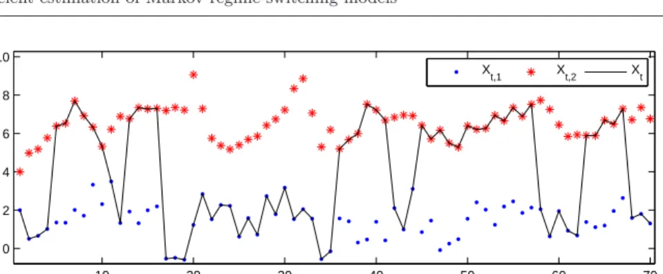
10 20 30 40 50 60 70 0 2 4 6 8 10 Time Value X t,1 Xt,2 Xt

Fig. 2 A sample trajectory of a MRS model with independent regimes (black solid line) superimposed on the observable and latent values of the processes in both regimes. The simulation was performed for a model with the following parameters:p11= 0.9,p22= 0.8,

wherep(_ijn)is the transition probability from the previous iteration. All values obtained in the M-step are then used as a new parameter vector θ(n+1) ₌

(ˆαi,βî,σî,γî,P(n+1), ρ

(n+1)

i ),i= 1,2, in the next iteration of the E-step.

3.2 Independent regimes variant

In the parameter-switching model (3) the current value of the process depends on the last observation only, no matter which regime it originated from. This implies that for the calculation of the conditional pdf (6), used in the i) part of the E-step recursions, the information from only one preceding time step is needed. Consequently, the EM algorithm requires storing conditional proba-bilitiesP(Rt=i|xT) of one time step only, i.e. 2T values in total.

However, the estimation procedure complicates significantly, if the regimes are independent from each other. Observe, that the values of the mean-re-verting regime become latent when the process is in the other state (see Figure 2 for an illustration). This makes the distribution of Xt dependent

(9)

possible paths of the state process (R1, R2, ..., Rt) should be considered in

the estimation procedure, implying that f(xt|Rt = i, Rt−1 6= i, ..., Rt−j 6=

i, Rt−j−1=i;xt−1;θ(n)) and the whole set of probabilitiesP(Rt=it, Rt−1=

it−1, ..., Rt−j =it−j|xt−1;θ(n)) should be used in the E-step. Obviously, this

leads to a high computational complexity, as the number of possible state pro-cess realizations is equal to 2T _{and increases rapidly with sample size. To be}

more precise, the total number of probabilities required by the EM algorithm to be stored in computer memory is equal to 2(2T+1₋_{1). Assuming that each}

probability is stored as a double precision floating-point number (8 bytes), estimating parameters from a sample of T = 30 observations would require 32 gigabytes of memory! For samples of typical size (a few hundred to a few thousand observations) this is clearly impossible with today’s computers.

As a feasible solution to this problem Huisman and de Jong (2002) sug-gested to use probabilities of the last 10 observations. Apart from the fact that such an approximation still is computationally intensive (requires storing 2{210₍_T₋₉₎₋₁_}_{probabilities in computer memory), it can be used only if the}

probability of more than 10 consecutive observations from the second (spike) regime is negligible. In Section 4 we will perform a simulation study to see how limiting is this theoretical assumption in practice.

Instead, in this article we suggest to replace the latent variables xt−1 in

formula (6) with their expectations ˜xt−1 =E(Xt−1|xt−1;θ(n)) based on the

whole information available at time t₋1. A similar approach was used by Gray (1996) in the context of regime-switching GARCH models to avoid the problem of the conditional standard deviation path dependence. Now, the estimation procedure described in Section 3.1 can be applied with the following approximation of the pdf: fxt|Rt=i;xt−1;θ(n) = _√ 1 2πσ_i(n)|x˜t−1,i|γ (n) i · ·exp      − xt− 1−β(_in)x˜t−1,i−α (n) i 2 2σ(_in)2_|x˜t−1,i|2γi (n)      , (11)

where ˜xt,i denotes the expected value of the ith regime at time t, that is

E Xt,i|xt;θ(n)

. Note, that compared to formula (6) for the parameter-switch-ing variant, the observed value of the process xt−1 is now replaced by the

expected value ˜xt−1,i of the ith regime at time t−1. The expected values

˜

xt,i=E Xt,i|xt;θ(n)can be computed using the following recursive formula

(for the derivation see the Appendix):

EXt,i|xt;θ(n) =PRt=i|xt;θ(n) xt+P Rt6=i|xt;θ(n) · (12) ·nα(_in)+1−β_i(n)EXt−1,i|xt−1;θ(n) o .

(10)

It is interesting to note, that EXt,i|xt;θ(n) = t−1 X k=0 xt−k 1−β_i(n) k PRt−k=i|xt−k;θ(n) · · k Y j=1 PRt−j+16=i|xt−j+1;θ(n) + +α(_in) t−1 X k=0 1−β_i(n)k k Y j=0 PRt−j+16=i|xt−j+1;θ(n) .

Hence, the expected value E(Xt,i|xt;θ(n)) is a linear combination of the

ob-served vector xt and the probabilities P(Rj = i|xj;θ(n)) calculated during

the estimation procedure (see the filtering part of the E-step). This observa-tion shows that using ˜xt−1,i=E(Xt−1,i|xt−1;θ(n)) in formula (11) instead of

xt−1, as in formula (6) for the parameter-switching variant, the computational

complexity of the E-step is greatly reduced. In particular, in the proposed modification of the EM algorithm the total number of probabilities stored in computer memory is only 4T. This means that for a sample ofT = 30 observa-tions only 1 kilobyte of memory is required, compared to 335 kilobytes in the approach utilizing probabilities of the last 10 observations and 32 gigabytes in the standard EM algorithm.

The estimation procedure described in this section can be applied to models in which at least one regime is described by the mean-reverting process given by (5). The independent regimes specification is commonly used in the elec-tricity price modeling literature (for a recent review see Janczura and Weron, 2010). It is often assumed that one regime follows a mean-reverting process, while the values in the other regime(s) are independent random variables from a specified distribution. The estimation steps are then as described above, with the exception that the M-step is now dependent on the choice of the distribu-tion in the other regime(s). Finally, note that in MRS models the likelihood function should be weighted with the corresponding probability, analogously as in the derivation of estimates (7)-(9) in the parameter-switching variant.

4 Simulation study

In order to test the performance of the estimation method proposed in Section 3.2, we provide a simulation study. For each of the following three MRS model types we generate 1000 sample trajectories:

– MR: with parameter-switching mean-reverting regimes, see (3),

– IMR: with independent mean-reverting processes in both regimes, see (5),

– IMR-G: with a mean-reverting process in the first regime and independent N(α2, σ22)-distributed random variables in the second regime.

(11)

Table 1 Means, 95% conﬁdence intervals (CIl,CIu) and standard deviations (Std) of

pa-rameter estimates obtained from 1000 simulated trajectories of 10000 observations each, for the three studied MRS model types: MR, IMR, and IMR-G.

α1 β1 σ2₁ γ1 α2 β2 σ2₂ γ2 p11 p22 MR True 1.0000 0.7000 1.0000 0.0000 2.0000 0.3000 0.0100 1.0000 0.5000 0.5000 Mean 1.0006 0.7001 1.0004 -0.0002 2.0000 0.3000 0.0100 1.0010 0.4998 0.4993 CI_l 0.9493 0.6842 0.9504 -0.0223 1.9997 0.2974 0.0094 0.9752 0.4854 0.4856 CIu 1.0587 0.7157 1.0543 0.0223 2.0003 0.3026 0.0106 1.0251 0.5134 0.5128 Std 0.0332 0.0095 0.0316 0.0137 0.0002 0.0016 0.0004 0.0152 0.0083 0.0081 IMR True 1.0000 0.7000 1.0000 0.0000 2.0000 0.3000 0.0100 1.0000 0.9000 0.8000 Mean 0.9974 0.6973 1.0135 0.0029 1.9702 0.2957 0.0128 1.0010 0.9004 0.8003 CI_l 0.9633 0.6778 0.9836 -0.0126 1.8347 0.2753 0.0026 0.8219 0.8941 0.7892 CIu 1.0339 0.7189 1.0435 0.0176 2.1145 0.3181 0.0496 1.1716 0.9066 0.8113 Std 0.0216 0.0126 0.0184 0.0094 0.0857 0.0131 0.0055 0.1051 0.0038 0.0068 IMR-G True 1.0000 0.7000 0.5000 0.5000 7.0000 0.5000 0.8000 0.000 Mean 0.9999 0.7009 0.5074 0.5036 6.9959 0.5063 0.7999 0.2018 CI_l 0.9893 0.6888 0.4924 0.4865 6.9689 0.4801 0.7928 0.1876 CIu 1.0113 0.7136 0.5220 0.5209 7.0218 0.5348 0.8071 0.2163 Std 0.0067 0.0075 0.0087 0.0105 0.0160 0.0165 0.0044 0.0089

Table 2 Means and standard deviations (Std), over 1000 simulated trajectories, of param-eter estimates in the MR model calculated for diﬀerent sample sizes.

α1 β1 σ12 γ1 α2 β2 σ22 γ2 p11 p22 True 1.0000 0.7000 1.0000 0.0000 2.0000 0.3000 0.0100 1.0000 0.5000 0.5000 Size Mean 100 0.9904 0.7040 0.8863 0.0455 1.9990 0.3011 0.0088 1.1214 0.4895 0.4962 500 1.0027 0.7000 0.9818 0.0069 2.0000 0.2999 0.0096 1.0201 0.4986 0.4986 1000 1.0034 0.7014 0.9915 0.0021 2.0002 0.3002 0.0097 1.0151 0.4990 0.4989 2000 1.0021 0.7009 0.9966 0.0026 2.0000 0.3000 0.0099 1.0045 0.5002 0.4990 5000 1.0003 0.7003 0.9958 0.0005 2.0000 0.3000 0.0099 1.0035 0.4998 0.5000 10000 1.0006 0.7001 1.0004 -0.0002 2.0000 0.3000 0.0100 1.0010 0.4998 0.4993 Size Std 100 0.3746 0.1111 0.3903 0.2280 0.0279 0.0219 0.0056 0.2797 0.0864 0.0865 500 0.1563 0.0461 0.1535 0.0703 0.0042 0.0077 0.0018 0.0766 0.0350 0.0362 1000 0.1094 0.0311 0.1035 0.0453 0.0020 0.0051 0.0013 0.0518 0.0263 0.0256 2000 0.0719 0.0214 0.0719 0.0298 0.0010 0.0035 0.0008 0.0335 0.0179 0.0180 5000 0.0474 0.0139 0.0455 0.0196 0.0004 0.0023 0.0005 0.0213 0.0115 0.0115 10000 0.0332 0.0095 0.0316 0.0137 0.0002 0.0016 0.0004 0.0152 0.0083 0.0081

The IMR model is simulated with probabilities of staying in the same regime equal to p11 = 0.9 and p22 = 0.8 for the first and the second regime,

re-spectively. With such a choice of the transition matrix we can expect to see many consecutive observations in each regime. Indeed, the probability of 10 consecutive observations from the first regime is equal to 0.35 and even for 40 consecutive observations that probability is still higher than 0.01. Obviously, such a model cannot be estimated based on the information about only a few prevailing observations.

For each sample trajectory we apply one of the estimation procedures de-scribed in Section 3. Then, we calculate the means, standard deviations and 95% confidence intervals of the parameter estimates. The values obtained for trajectories consisting of 10000 observations are given in Table 1. All sample means are close to the true parameters with a deviation of no more than 0.03 (in absolute terms). In fact, in most cases the deviation is significantly lower. Moreover, all parameter values are within the obtained 95% confidence inter-vals. Also the standard deviation of the estimates is quite low and, except for

γ2andα2 in the IMR model, does not exceed 0.04.

Next, we check how the proposed method works for different sample sizes. We generate MRS model trajectories with 100, 500, 1000, 2000, 5000, and

(12)

0 2000 4000 6000 8000 10000 0.5 1 1.5 α1 Sample size 0 2000 4000 6000 8000 10000 0.5 0.6 0.7 0.8 0.9 β1 Sample size 0 2000 4000 6000 8000 10000 0.5 1 1.5 σ 2 1 Sample size 0 2000 4000 6000 8000 10000 −0.2 0 0.2 0.4 γ1 Sample size 0 2000 4000 6000 8000 10000 1.99 2 2.01 α2 Sample size 0 2000 4000 6000 8000 10000 0.28 0.3 0.32 0.34 β2 Sample size 0 2000 4000 6000 8000 10000 0 0.01 0.02 σ 2 2 Sample size 0 2000 4000 6000 8000 10000 0.8 1 1.2 1.4 1.6 γ2 Sample size 0 2000 4000 6000 8000 10000 0.4 0.5 0.6 p11 Sample size 0 2000 4000 6000 8000 10000 0.4 0.5 0.6 p22 Sample size

Fig. 3 95% conﬁdence intervals of parameter estimates in the MRS model with parameter-switching mean-reverting regimes (MR; see Table 1 for parameter details). The true param-eter values are given by the solid red lines.

Table 3 Means and standard deviations (Std), over 1000 simulated trajectories, of param-eter estimates in the IMR model calculated for diﬀerent sample sizes.

α1 β1 σ₁2 γ1 α2 β2 σ2₂ γ2 p11 p22 True 1.0000 0.7000 1.0000 0.0000 2.0000 0.3000 0.0100 1.0000 0.9000 0.8000 Size Mean 100 1.0221 0.7280 0.9765 0.0298 2.6473 0.3982 22647 1.0580 0.8951 0.7798 500 1.0002 0.7026 1.0109 0.0061 2.0368 0.3057 0.5569 0.9822 0.8997 0.7956 1000 1.0037 0.7025 1.0070 0.0075 2.0319 0.3052 0.0391 0.9995 0.9004 0.7981 2000 0.9992 0.6987 1.0130 0.0024 1.9781 0.2969 0.0200 1.0046 0.9006 0.7993 5000 1.0001 0.6988 1.0128 0.0044 1.9615 0.2944 0.0139 1.0059 0.9004 0.8001 10000 0.9974 0.6973 1.0135 0.0029 1.9702 0.2957 0.0128 1.0010 0.9004 0.8003 Size Std 100 0.2254 0.1358 0.1975 0.1341 1.3062 0.1986 71587 2.1783 0.0385 0.0779 500 0.0954 0.0558 0.0869 0.0487 0.4207 0.0641 9.0870 0.5930 0.0166 0.0318 1000 0.0668 0.0403 0.0601 0.0312 0.2917 0.0444 0.1958 0.3687 0.0116 0.0218 2000 0.0473 0.0275 0.0408 0.0211 0.2006 0.0306 0.0620 0.2397 0.0083 0.0156 5000 0.0296 0.0176 0.0263 0.0135 0.1213 0.0184 0.0093 0.1606 0.0052 0.0098 10000 0.0216 0.0126 0.0184 0.0094 0.0857 0.0131 0.0055 0.1051 0.0038 0.0068

(13)

0 2000 4000 6000 8000 10000 0.8 1 1.2 1.4 α1 Sample size 0 2000 4000 6000 8000 10000 0.4 0.6 0.8 1 β1 Sample size 0 2000 4000 6000 8000 10000 0.8 1 1.2 σ 2 1 Sample size 0 2000 4000 6000 8000 10000 −0.2 0 0.2 γ1 Sample size 0 2000 4000 6000 8000 10000 1 2 3 4 5 α2 Sample size 0 2000 4000 6000 8000 10000 0.2 0.4 0.6 0.8 β2 Sample size 0 2000 4000 6000 8000 10000 0 0.05 0.1 0.15 σ 2 2 Sample size 0 2000 4000 6000 8000 10000 −2 0 2 4 γ2 Sample size 0 2000 4000 6000 8000 10000 0.85 0.9 0.95 p11 Sample size 0 2000 4000 6000 8000 10000 0.7 0.8 0.9 p22 Sample size

Fig. 4 95% conﬁdence intervals of parameter estimates in the MRS model with independent mean-reverting regimes (IMR; see Table 1 for parameter details). The true parameter values are given by the solid red lines.

Table 4 Means and standard deviations (Std), over 1000 simulated trajectories, of param-eter estimates in the IMR-G model calculated for diﬀerent sample sizes.

α1 β1 σ2₁ γ1 α2 σ2₂ p11 p22 True 1.0000 0.7000 0.5000 0.5000 7.0000 0.5000 0.8000 0.2000 Size Mean 100 1.0017 0.7002 0.5064 0.5876 7.0084 0.4732 0.7977 0.1889 500 1.0045 0.7048 0.5058 0.5221 7.0007 0.5068 0.8011 0.2008 1000 0.9997 0.7004 0.5066 0.5137 6.9941 0.5066 0.7995 0.2012 2000 1.0007 0.7012 0.5086 0.5071 6.9971 0.5038 0.8001 0.2020 5000 1.0000 0.7000 0.5072 0.5055 6.9955 0.5068 0.8001 0.2019 10000 0.9999 0.7009 0.5074 0.5036 6.9959 0.5063 0.7999 0.2018 Size Std 100 0.1021 0.0927 0.1062 0.1622 0.1617 0.1730 0.0442 0.0910 500 0.0380 0.0370 0.0403 0.0563 0.0755 0.0786 0.0194 0.0395 1000 0.0252 0.0257 0.0273 0.0374 0.0510 0.0545 0.0147 0.0277 2000 0.0165 0.0174 0.0189 0.0251 0.0362 0.0377 0.0100 0.0192 5000 0.0098 0.0113 0.0121 0.0153 0.0232 0.0235 0.0065 0.0127 10000 0.0067 0.0075 0.0087 0.0105 0.0160 0.0165 0.0044 0.0089

(14)

0 2000 4000 6000 8000 10000 0.9 1 1.1 α1 Sample size 0 2000 4000 6000 8000 10000 0.6 0.7 0.8 β1 Sample size 0 2000 4000 6000 8000 10000 0.4 0.5 0.6 0.7 σ 2 1 Sample size 0 2000 4000 6000 8000 10000 0.4 0.6 0.8 γ1 Sample size 0 2000 4000 6000 8000 10000 6.8 7 7.2 α2 Sample size 0 2000 4000 6000 8000 10000 0.2 0.4 0.6 σ 2 2 Sample size 0 2000 4000 6000 8000 10000 0.75 0.8 0.85 p11 Sample size 0 2000 4000 6000 8000 10000 0.1 0.2 0.3 p22 Sample size

Fig. 5 95% conﬁdence intervals of parameter estimates in the MRS model with a mean-reverting regime combined with independent Gaussian random variables (IMR-G; see Table 1 for parameter details). The true parameter values are given by the solid red lines.

10000 observations. The obtained means and standard deviations are given in Tables 2 (MR model), 3 (IMR model) and 4 (IMR-G model). The respective confidence intervals are plotted in Figures 3, 4 and 5. As expected, the stan-dard deviations, as well as, the width of the confidence intervals decrease with increasing sample size. Looking at the means, in most cases a sample of 1000 (or even 500 for the MR and IMR-G models) observations yields satisfactory results, as the deviation does not exceed 0.03 (in absolute terms). Especially for the IMR-G model the results are very satisfactory. This is important in view of the fact that a variant of this model is used in Section 5 for modeling electricity spot prices.

Finally, we compare the convergence of the proposed algorithm (in what follows called method I) with the approach utilizing probabilities of the last 10 observations (method II; as proposed by Huisman and de Jong, 2002). Observe, that since the conditional distributionf(xt|xt−k) of the process defined by (5)

is not known for a general value ofγifk >1, the latter method cannot be used in this case. Therefore, we limit the comparison of the two estimation methods to specifications with γ = 0. For 100 simulated trajectories of the IMR-G model we calculate the mean absolute errors (MAE) of the parameter estimates obtained from both approaches. We consider five sample sizes (100, 500, 1000, 2000 and 5000) and two sets of parameters: one with a low probability of

(15)

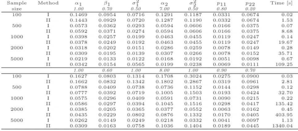
Table 5 Mean absolute errors (MAE) of the parameter estimates in the IMR-G model obtained from two estimation methods: the algorithm proposed in this paper (method I) and the approach utilizing probabilities of the last 10 observations (method II). The errors were computed over 100 simulations for each sample size and each set of parameters. The true (simulated) parameter values are given in italics. Additionally, the mean estimation times (in seconds) are provided in the last column.

Sample Method α1 β1 σ2₁ α2 σ2₂ p11 p22 Time [s]

size 1.00 0.70 0.50 7.00 0.50 0.80 0.20 100 I 0.1469 0.0954 0.0716 0.1291 0.1187 0.0331 0.0674 0.02 II 0.1443 0.0929 0.0720 0.1287 0.1190 0.0332 0.0674 1.53 500 I 0.0573 0.0362 0.0293 0.0594 0.0606 0.0166 0.0375 0.07 II 0.0592 0.0371 0.0274 0.0594 0.0606 0.0166 0.0375 8.68 1000 I 0.0398 0.0257 0.0199 0.0463 0.0455 0.0119 0.0247 0.14 II 0.0378 0.0249 0.0192 0.0463 0.0455 0.0119 0.0247 19.67 2000 I 0.0318 0.0202 0.0151 0.0286 0.0259 0.0078 0.0149 0.28 II 0.0309 0.0195 0.0139 0.0307 0.0266 0.0078 0.0152 35.71 5000 I 0.0219 0.0133 0.0122 0.0168 0.0192 0.0051 0.0098 0.67 II 0.0342 0.0154 0.0565 0.0199 0.0238 0.0069 0.0111 109.25 1.00 0.60 1.00 8.00 1.00 0.90 0.70 100 I 0.1627 0.0803 0.1314 0.1708 0.3024 0.0275 0.0900 0.03 II 0.1662 0.0832 0.1342 0.1802 0.2867 0.0319 0.0961 2.81 500 I 0.0788 0.0409 0.0738 0.0736 0.1152 0.0144 0.0298 0.12 II 0.0777 0.0392 0.0719 0.1005 0.1503 0.0193 0.0424 32.70 1000 I 0.0575 0.0296 0.0409 0.0591 0.0731 0.0090 0.0215 0.22 II 0.0586 0.0297 0.0394 0.1045 0.1516 0.0298 0.0417 135.42 2000 I 0.0385 0.0205 0.0365 0.0377 0.0552 0.0063 0.0162 0.45 II 0.0435 0.0229 0.0802 0.0876 0.1332 0.0170 0.0405 403.95 5000 I 0.0262 0.0149 0.0249 0.0218 0.0332 0.0041 0.0097 1.13 II 0.0309 0.0163 0.0758 0.1036 0.1404 0.0189 0.0445 1340.04

staying in the Gaussian regime (i.e. withp22= 0.2, so that the probability of

more than 10 consecutive observations from the Gaussian regime is less than 10−7 _{and, hence, can be neglected) and a second one with} _p

22 = 0.7. The

results are summarized in Table 5.

The mean absolute errors obtained for the first parameter set (withp22=

0.2) are comparable for both methods. However, if the probability of staying in the Gaussian regime for more than 10 consecutive observations is not negli-gible, method I apparently outperforms method II. The difference is especially noticeable for the Gaussian regime parameters (α2 and σ22) and the

transi-tion probabilities. Observe, that for samples of 5000 observatransi-tions the MAE obtained using method II are almost five times larger than the ones result-ing from usresult-ing method I. Moreover, while the errors decrease with increasresult-ing sample size when using method I, this is not observed for method II, e.g. for the estimates ofα2the MAE values are 0.1005, 0.1045, 0.0876 and 0.1036 for

samples of 500, 1000, 2000 and 5000 observations, respectively.

This simple simulation study shows the appealing efficiency of the esti-mation algorithm proposed in this article (method I), when compared to its competitor (method II). It also makes clear that method II can be used only if the probability of more than 10 consecutive observations from the spike (here Gaussian) regime can be ignored. Furthermore, compared to method I, method II is much more computationally demanding. In the last column of Table 5 we provide the mean (over 100 simulations) estimation times obtained using both approaches. Observe the striking difference between the two methods. Method I was found to be 100 to over 1000 times faster than method II (1.13s vs. 1340.04s)!

(16)

5 Application to electricity spot prices

In this study we present how the techniques introduced in Section 3 can be used to efficiently calibrate MRS models to electricity spot prices. We use mean daily (baseload) spot prices from two major power markets: the Euro-pean Energy Exchange (EEX; Germany) and the New South Wales Electricity Market (NSW; being part of the National Electricity Market in Australia). Us-ing baseload data is quite common in the energy economics literature, partly due to the fact that baseload is the most common underlying instrument for energy derivatives. The EEX sample totals 1820 daily observations (or 260 full weeks) and covers the roughly 5-year period January 2, 2006 – December 26, 2010. The NSW sample totals 1722 daily observations (246 full weeks) and covers the period January 2, 2006 – September 19, 2010. Recall that NSW is an ‘energy only market’, where the wholesale electricity price provides com-pensation for both variable and fixed costs (Weron, 2006). As a result, the observed prices are extremely spiky – they can reach up to 10000 AUD/MWh during peak hours and well over 1000 AUD/MWh in mean daily prices. On the other hand, a different generation stack with much less wind generation than in the EEX market yields no negative (or close to zero) prices. Conse-quently, in what follows we analyze NSW log-prices, i.e. natural logarithms of spot prices, which are more prone to modeling with the models studied in this article than the prices themselves.

When modeling electricity spot prices we have to bear in mind that electric-ity is a very specific commodelectric-ity. Both electricelectric-ity demand and (to some extent) supply exhibit seasonal fluctuations. They mostly arise due to changing cli-mate conditions, like temperature and the number of daylight hours. These seasonal fluctuations translate into seasonal behavior of electricity prices, and spot prices in particular. In the mid- and long-term also the fuel price levels (of natural gas, oil, coal) influence electricity prices. However, not wanting to focus the paper on modeling the fuel stack/bid stack/electricity spot price relationships, we use a single non-parametric long-term seasonal component (LTSC) to represent the long-term non-periodic fuel price levels, the changing climate/consumption conditions throughout the years and strategic bidding practices. An empirical justification for such an approach can be found, for in-stance, in Janczura and Weron (2010); see also Eydeland and Wolyniec (2003) and Karakatsani and Bunn (2010) for discussions on fundamental and behav-ioral drivers of electricity prices.

We assume that the electricity spot price (or log-price for the NSW power market), Pt, can be represented by a sum of two independent parts: a

pre-dictable (seasonal) componentft and a stochastic componentXt , i.e. Pt=

ft+Xt. Further, we let ft be composed of a weekly periodic part, st, and

a LTSC, Tt. The deseasonalization is then conducted in three steps. First,

the long term trendTtis estimated from daily spot pricesPtusing a wavelet

filtering-smoothing technique (for details see Tr¨uck et al., 2007; Weron, 2006). This procedure, also known as low pass filtering, yields a traditional linear smoother. Here we use the S6 approximation, which roughly corresponds to

(17)

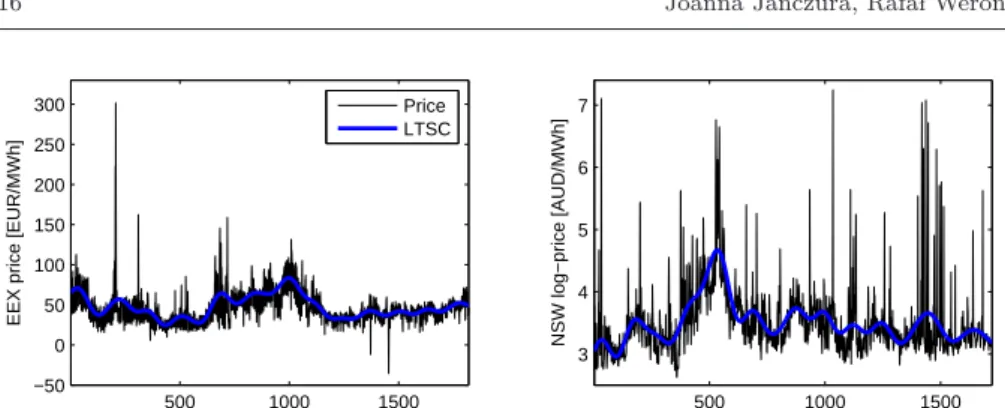
500 1000 1500 −50 0 50 100 150 200 250 300

EEX price [EUR/MWh]

Days [January 2, 2006 − December 26, 2010] Price LTSC 500 1000 1500 3 4 5 6 7 NSW log−price [AUD/MWh]

Days [January 2, 2006 − September 19, 2010]

Fig. 6 Mean daily spot EEX prices (left panel) and NSW log-prices (right panel) and the estimated long-term seasonal components (LTSC; thick blue lines).

bi-monthly (26_{= 64 days) smoothing. The estimated long term seasonal}

com-ponents are plotted in Figure 6.

Although forecasting is not the focus of this article, let us briefly comment on forecasting the trend-seasonal patterns. Predicting the LTSC beyond the next few days or weeks is a very difficult task. And wavelets are not very help-ful in this context. Unlike sines and cosines, individual wavelet functions are quite localized in time or (more generally) in space. For the lower detail levels of the wavelet decomposition, which are of high frequency and oscillatory in nature, a trigonometric (Yousefi et al., 2005) or an ARIMA (Conejo et al., 2005) fit can be used. However, for the much smoother approximation level (e.g. theS6 approximation in our case) and the higher detail levels rather a

spline fit (Yousefi et al., 2005) or a polynomial extrapolation (Wong et al., 2003) is applied to extend the signal. Naturally, the choice of the extrapola-tion method and the range of values used for calibraextrapola-tion is subjective and, hence, the LTSC forecasts will most likely diverge for different methods. As mentioned by Janczura and Weron (2010), a potentially promising, alterna-tive approach would be to use forward looking information, like smoothed forward curves (Benth et al., 2007; Borak and Weron, 2008). The information carried by forward prices provides insights as to the future evolution of spot prices. However, forward prices also include the risk premium (Benth et al., 2008; Weron, 2008), which should somehow be separated from the spot price forecast for it to be useful.

The price series without the LTSC is obtained by subtracting the S6

ap-proximation fromPt. Next, the weekly periodicitystis removed by subtracting

the ‘average week’ calculated as the median of prices corresponding to each day of the week (the median is used instead of the mean due to its robustness against outliers – the extremely spiky prices, especially in NSW data). Finally, the deseasonalized prices, i.e.Pt−Tt−st, are shifted so that the mean of the

new process is the same as the mean ofPt. The resulting deseasonalized time

(18)

The second well known feature of electricity prices are the sudden, unex-pected price changes, known as spikes or jumps. The ‘spiky’ nature of spot prices is the effect of non-storability of electricity. Electricity to be delivered at a specific hour cannot be substituted for electricity available shortly after or before. Extreme load fluctuations – caused by severe weather conditions often in combination with generation outages or transmission failures – can lead to price spikes. On the other hand, an oversupply – due to a sudden drop in demand and technical limitations of an instant shut-down of a generator – can cause price drops. Further, electricity spot prices are in general regarded to be mean-reverting and exhibit the so called ‘inverse leverage effect’, meaning that the positive shocks increase volatility more than the negative shocks. Knittel and Roberts (2005) attributed this phenomenon to the fact that a positive shock to electricity prices can be treated as an unexpected positive demand shock. Therefore, as a result of convex marginal costs, positive demand shocks have a larger impact on price changes relative to negative shocks.

Motivated by these features of electricity spot prices we let the stochas-tic component Xt be driven by a Markov regime-switching model with three

independent states: Xt=    Xt,1 ifRt= 1, Xt,2 ifRt= 2, Xt,3 ifRt= 3. (13) The first (base) regime describes the ‘normal’ price behavior and is given by the mean-reverting, heteroskedastic process of the form:

Xt,1=α1+ (1−β1)Xt−1,1+σ1|Xt−1,1|γ1ǫt, (14)

where ǫt is the standard Gaussian noise. The second regime represents the

sudden price jumps (spikes) caused by unexpected supply shortages and is given by i.i.d. random variables from the shifted log-normal distribution:

log(Xt,2−X(q2))∼N(α2, σ22), Xt,2> X(q2). (15)

Finally, the third regime (responsible for the sudden price drops) is governed by the shifted ‘inverse log-normal’ law:

log(−Xt,3+X(q3))∼N(α3, σ23), Xt,3< X(q3). (16)

It turns out that, unlike EEX prices, NSW prices do not exhibit significant price drops, even on the log-scale. A third regime is not needed to adequately model the dynamics. Hence, in what follows we fit a 2-regime model (without a price drop regime) to the deseasonalized NSW log-prices.

In the above formulas X(qi) denotes the qi-quantile, qi ∈ (0,1), of the

dataset. Generally the choice ofqi is arbitrary, however, in this paper we let

q2= 0.75 andq3= 0.25, i.e. the third and the first quartile, respectively. This is

motivated by the statistical properties of the model in which small fluctuations are driven by the base regime dynamics. Only the large deviations should be driven by the spike or drop regime dynamics.

(19)

0 200 400 600 800 1000 1200 1400 1600 1800 0

100 200 300

EEX price [EUR/MWh]

Base Spike Drop 0 200 400 600 800 1000 1200 1400 1600 1800 0 0.5 1 P(S) 0 200 400 600 800 1000 1200 1400 1600 1800 0 0.5 1 P(D)

Days [January 2, 2006 − December 26, 2010]

Fig. 7 Calibration results of a MRS model with three independent regimes ﬁtted to the deseasonalized EEX prices. The lower panels display the conditional probabilitiesP(S) = P(Rt = 2|x₁, x₂, ..., xT) and P(D) = P(Rt = 3|x₁, x₂, ..., xT) of being in the spike or

drop regime, respectively. The prices classiﬁed as spikes or drops, i.e. withP(S)>0.5 or P(D)>0.5, are denoted by dots or ‘x’ in the upper panel.

0 200 400 600 800 1000 1200 1400 1600 3 4 5 6 7 8 NSW log−price [AUD/MWh] Base Spike 0 200 400 600 800 1000 1200 1400 1600 0 0.5 1 P(S)

Days [January 2, 2006 − September 19, 2010]

Fig. 8 Calibration results of a MRS model with two independent regimes ﬁtted to the deseasonalized NSW log-prices. The lower panel displays the conditional probabilityP(S) of being in the spike regime. The prices classiﬁed as spikes, i.e. withP(S)>0.5, are denoted by dots in the upper panel.

The deseasonalized prices Xt and the conditional probabilities of being

in the spike P(Rt = 2|x1, x2, ..., xT) or drop P(Rt = 3|x1, x2, ..., xT) regime

for the analyzed datasets are displayed in Figures 7 and 8. The prices clas-sified as spikes or drops, i.e. with P(Rt = 2|x1, x2, ..., xT) > 0.5 or P(Rt =

3|x1, x2, ..., xT)>0.5, are additionally denoted by dots or ‘x’. The estimated

model parameters are given in Table 6.

The obtained base regime parameters are consistent with the well known properties of electricity prices. In particular,β1∈[0.20,0.44] indicates a

(20)

Table 6 Calibration results for MRS models with (two or three) independent regimes ﬁtted to the deseasonalized EEX prices and NSW log-prices.

Parameters Probabilities

α1 β1 σ2₁ γ1 α2 σ2₂ α3 σ2₃ p11 p22 p33

EEX 14.08 0.44 7.23 0.18 2.34 0.87 2.49 0.33 0.9270 0.6420 0.6603

NSW 0.67 0.20 4e-4 1.60 -0.99 1.40 - - 0.9539 0.6390

-Table 7 Goodness-of-fit statistics for MRS models fitted to the deseasonalized EEX prices and NSW log-prices. For quantiles the relative differences between the sample and the model implied statistics are given (the latter were obtained from 100 simulations).

Quantiles K-S testp-values

0.1 0.25 0.5 0.75 0.9 Base Spike Drop Model

EEX -0.8% -0.6% -0.3% 0.2% 0.5% 0.50 0.26 0.69 0.31

NSW -0.2% -0.8% -0.3% 0.8% 0.7% 0.09 0.33 - 0.18

for the ‘inverse leverage effect’. Finally, considering probabilitiespii of staying

in the same regime we obtain quite high values for each of the regimes, rang-ing from 0.6390 for the spike regime in the NSW market up to 0.9539 for the base regime in the same market. As a consequence, on average there are many consecutive observations from the same regime.

In order to check the statistical adequacy of the fitted MRS models we cal-culate percentage differences between the data and the model implied quan-tiles, see Table 7. The model implied values are obtained as the mean value of the statistics calculated over 100 simulated trajectories. A negative sign indi-cates that the value obtained from the dataset is lower than the model-implied. Observe that all differences between the data and the model-implied statistics are less than 0.8%, which indicates a relatively good fit of the models.

Moreover, we report thep-values of a Kolmogorov-Smirnov (K-S) goodness-of-fit type test for each of the individual regimes, as well as, for the whole model (for test details see Janczura and Weron, 2011). The goodness-of-fit results are summarized in Table 7. All K-S test p-values are higher than the commonly used 5% significance level, hence we cannot reject the hypotheses that the datasets follow the fitted MRS models.

6 Conclusions

In this paper we have proposed a method that greatly reduces the compu-tational burden induced by the introduction of independent regimes in MRS models. Instead of storing conditional probabilities for each of the possible state process paths, our method requires conditional probabilities for only one time-step. This allows for a 100 to over 1000 times faster calibration than in case of a competing approach utilizing probabilities of the last 10 observations (see Table 5). Our method is also more general and admits any value of γ in the base regime dynamics.

We have further performed a limited simulation study to test the accuracy of the new method and applied it to sample series of electricity spot prices. The simulation study has shown that all sample means are close to the true parameter values (and all true parameter values are within the obtained 95%

(21)

confidence intervals). Looking at the means, in most cases a sample of 1000 (or even 500 for the MR and IMR-G models; for model acronyms and definitions see Section 4) observations yields satisfactory results, as the deviation does not exceed 0.03 (in absolute terms). Especially for the IMR-G model the results are very satisfactory. This is important in view of the fact that variants of this model are popular in the energy economics literature. In particular, a model of this type is calibrated in Section 5 to sample series of deseasonalized wholesale prices from the German EEX and Australian NSW markets. The model fits market data well and also replicates the major stylized facts of electricity spot price dynamics. In particular, the parameterγ can be treated as a parameter representing the ‘degree of inverse leverage’. A positive value (e.g. 0.18 or 1.60 as in Table 6) indicates ‘inverse leverage’, which reflects the observation that positive electricity price shocks increase volatility more than negative shocks. Finally, since MRS models can be considered as generalizations of HMMs, the results of this paper can have far-reaching implications for many problems where HMMs have been applied (see e.g. Mamon and Elliott, 2007). In some cases, perhaps, a MRS model with independent regimes would constitute a more realistic model of the observed phenomenon than a HMM.

Acknowledgments

We thank Tomasz Piesiewicz of TAURON Polska Energia and Stefan Tr¨uck of Macquarie University for electricity spot price data. This paper has benefited from conversations with the participants of the DStatG 2010 Annual Meeting, the Trondheim Summer 2011 Energy Workshop, the 2011 WPI Conference in Energy Finance and the seminars at Macquarie University, University of Sydney and University of Verona. J.J. acknowledges partial financial support from the European Union within the European Social Fund. The work of R.W. was partially supported by ARC grant no. DP1096326.

Appendix

The recursive formula (12) can be derived in the following way. Let Xt =

(X1, X2, ..., Xt). Observe that

Xt,i=IRt=iXt+IRt6=i[αi+ (1−βi)Xt−1,i+σi|Xt−1,i|

γi_ǫ

t], (17)

where Ix is the indicator function. Taking the expected value conditional on

(22)

SinceXt−1,iandǫtare independent of theσ-algebra generated by{Xt, Rt6=i} we have E_|Xt−1,i|γ (n) i ǫ t|Xt, Rt6=i;θ(n) =E_|Xt−1,i|γ (n) i ǫ t|Xt−1;θ(n) , and EXt−1,i|Xt, Rt6=i;θ(n) =EXt−1,i|Xt−1;θ(n) .

Moreover, from the law of iterated expectation and basic properties of condi-tional expected values:

Finally, substituting the variablesXt with their observationsxt leads to

for-mula (12).

References

Benth, F.E., Benth, J.S., Koekebakker, S. (2008). Stochastic Modeling of Electricity and Related Markets. World Scientiﬁc, Singapore.

Benth, F.E., Cartea, A., Kiesel, R. (2008). Pricing forward contracts in power markets by the certainty equivalence principle: Explaining the sign of the market risk premium. Journal of Banking & Finance 32(10), 2006-2021.

Benth, F.E., Koekebakker, S., Ollmar, F. (2007). Extracting and applying smooth for-ward curves from average-based commodity contracts with seasonal variation. Journal of Derivatives – Fall, 52-66.

Bierbrauer, M., Menn, C., Rachev, S.T., Tr¨uck, S. (2007). Spot and derivative pricing in the EEX power market. Journal of Banking and Finance 31, 3462-3485.

Borak, S., Weron, R. (2008). A semiparametric factor model for electricity forward curve dynamics. Journal of Energy Markets 1(3), 3-16.

Cappe, O., Moulines E., Ryden T. (2005). Inference in Hidden Markov Models. Springer. Christensen, T., Hurn, S., Lindsay, K. (2009). It never rains but it pours: modeling the

persistence of spikes in electricity prices. The Energy Journal 30(1), 25-48.

Conejo, A.J., Plazas, M.A., Esp´ınola, R., Molina, A.B. (2005). Day-ahead electricity price forecasting using the wavelet transform and ARIMA models. IEEE Transactions on Power Systems 20(2), 1035-1042.

De Jong, C. (2006). The nature of power spikes: A regime-switch approach. Studies in Nonlinear Dynamics & Econometrics 10(3), Article 3.

Dempster, A., Laird, N., Rubin, D.B. (1977). Maximum likelihood from incomplete data via the EM algorithm. Journal of the Royal Statistical Society 39, 1-38.

(23)

Erlwein, C., Benth, F.E., Mamon, R. (2010). HMM ﬁltering and parameter estimation of an electricity spot price model. Energy Economics 32, 1034-1043.

Eydeland, A., Wolyniec, K. (2003). Energy and Power Risk Management. Wiley, Hoboken, NJ.

Fink, G.A. (2008). Markov Models for Pattern Recognition: From Theory to Applications. Springer.

Gray, S.F. (1996). Modeling the conditional distribution of interest rates as a regime-switching process. Journal of Financial Economics 42, 27-62.

Hahn, M., Fr¨uhwirth-Schnatter, S., Sass, J. (2009). Estimating models based on Markov jump processes given fragmented observation series. AStA 93, 403-425.

Hamilton, J. (1989). A new approach to the economic analysis of nonstationary time series and the business cycle. Econometrica 57, 357-384.

Hamilton, J. (1990). Analysis of time series subject to changes in regime. Journal of Econo-metrics 45, 39-70.

Hamilton, J. (1996) Regime switching models. In: The New Palgrave Dictionary of Eco-nomics (2nd ed.).

Huisman, R. (2009). An Introduction to Models for the Energy Markets. Risk Books. Huisman, R., de Jong, C. (2002). Option formulas for mean-reverting power prices with

spikes. ERIM Report Series Reference No. ERS-2002-96-F&A.

Huisman, R., Mahieu, R. (2003). Regime jumps in electricity prices. Energy Economics 25, 425-434.

Janczura, J., Weron, R. (2010). An empirical comparison of alternate regime-switching mod-els for electricity spot prices. Energy Economics 32, 1059-1073.

Janczura, J., Weron, R. (2011). Goodness-of-ﬁt testing for the marginal distribution of regime-switching models. Available at MPRA: http://mpra.ub.uni-muenchen.de/32532. Kanamura, T., ¯Ohashi, K. (2008). On transition probabilities of regime switching in

elec-tricity prices. Energy Economics 30, 1158-1172.

Karakatsani, N.V., Bunn, D.W. (2008). Intra-day and regime-switching dynamics in elec-tricity price formation. Energy Economics 30, 1776-1797.

Karakatsani, N.V., Bunn, D. (2010) Fundamental and behavioural drivers of electricity price volatility. Studies in Nonlinear Dynamics & Econometrics 14(4), Article 4.

Kholodnyi, V.A. (2005). Modeling power forward prices for power with spikes: A non-Markovian approach. Nonlinear Analysis 63, 958-965.

Kim, C.-J. (1994). Dynamic linear models with Markov-switching. Journal of Econometrics 60, 1-22.

Knittel, C.R., Roberts, M.R. (2005). An empirical examination of restructured electricity prices. Energy Economics 27, 791-817.

Luo, Q., Mao, X. (2007) Stochastic population dynamics under regime switching. Journal of Mathematical Analysis and Applications, 334(1), 69-84.

Mamon, R.S., Elliott, R.J., eds. (2007). Hidden Markov Models in Finance. International Series in Operations Research & Management Science, Vol. 104, Springer.

Mari, C. (2008). Random movements of power prices in competitive markets: A hybrid model approach. Journal of Energy Markets 1(2), 87-103.

Mount, T.D., Ning, Y., Cai, X. (2006). Predicting price spikes in electricity markets using a regime-switching model with time-varying parameters. Energy Economics 28: 62-80. Tr¨uck, S., Weron, R., Wolﬀ, R. (2007). Outlier treatment and robust approaches for modeling

electricity spot prices. Proceedings of the 56th Session of the ISI. Available at MPRA: http://mpra.ub.uni-muenchen.de/4711/.

Weron, R. (2006). Modeling and forecasting electricity loads and prices: A statistical ap-proach. Wiley, Chichester.

Weron, R. (2008) Market price of risk implied by Asian-style electricity options and futures. Energy Economics 30, 1098-1115.

Weron, R. (2009). Heavy-tails and regime-switching in electricity prices. Mathematical Methods of Operations Research 69(3), 457-473.

Wong, H., Ip, W.-C., Xie, Z., Lui, X. (2003) Modelling and forecasting by wavelets, and the application to exchange rates. Journal of Applied Statistics 30(5), 537-553.

Youseﬁ, S., Weinreich, I., Reinarz, D. (2005) Wavelet-based prediction of oil prices. Chaos, Solitons and Fractals 25, 265-275.