Stochastic Modeling for Commodity Prices andValuation of Commodity Derivatives under Stochastic Convenience Yields and Seasonality

(1)

INAUGURAL-DISSERTATION

zur

Erlangung der Doktorwürde

der

Naturwissenschaftlich-Mathematischen Gesamtfakultät

der

Ruprecht-Karls-Universität

Heidelberg

vorgelegt von

M.Sc..

-

Sanae Rujivan

aus Thailand

(2)

S

t

o

c

h

a

s

t

i

c

M

o

d

e

l

i

n

g

f

o

r

C

o

m

o

d

i

t

y

P

r

i

c

e

s

a

n

d

V

a

l

u

a

t

i

o

n

o

f

C

o

m

o

d

i

t

y

D

e

r

i

v

a

t

i

v

e

s

u

n

d

e

r

S

t

o

c

h

a

s

t

i

c

C

o

n

v

e

n

i

e

n

c

e

Y

i

e

l

d

s

a

n

d

S

e

a

s

o

n

a

l

i

t

y

Gutachter: Prof. Dr. Dr. h.c. mult. Willi Jäger

(3)

A

b

s

t

r

a

c

t

In this dissertation, we develop a two-factor model of the stochastic behavior of commodity prices. The first factor is the commodity spot price which follows a geometric Brownian motion with a time-varying volatility. The second factor is the instantaneous convenience yield which follows an extended Cox-Ingersoll-Ross (CIR) process by adding a time-dependent function into the drift term of the process in order to describe seasonal variations in commodity prices. The time-varying volatilities of the commodity spot prices and the instantaneous convenience yields are proportional to the square root of the instantaneous convenience yields. Our modeling concerns about two important things: a link between price volatilities and convenience yields as suggested by the theory of storage, and the seasonality in commodity prices and convenience yield volatilities. We establish sufficient conditions to guarantee the inaccessibility to nonpositive values of the volatility process. Closed-form solutions for futures prices are derived under the standard no-arbitrage arguments. The closed-form solutions are consistent with the theory of storage: futures prices tend to be lower than spot prices when convenience yields are sufficiently high and vice versa. In addition, the closed-form solutions lead to extraction formulas for the two factors under the assumption that two no-arbitrage futures prices having different maturities can be observed. Moreover, European futures options prices are determined by using a method of Fourier transforms. We estimate the model parameters using the daily futures prices data of two agricultural commodities in Thailand: rice and natural rubber. The futures prices data are obtained from the Agricultural Futures Exchange of Thailand (AFET) in sample periods in August 2004 to August 2006. The estimation method is based on a maximum likelihood approach. The empirical results are in accordance with the theory of storage and we have a comment on the Thai price intervention scheme. Using the estimated parameters, we calculate price differences and correlations between the observed futures prices and the predicted futures prices, obtained from our model, for several futures contracts of the two commodities. The results obtained show the observed and the predicted futures prices are insignificantly different and strongly positive correlated. Finally, we analyze the implications of our model for capital budgeting decisions by investigating the situations known as backwardation.I_and contango.II_{in AFET. We have found that, for long maturity futures contracts, the futures} market of rice exhibited backwardation, while the futures market of natural rubber exhibited contango.

Keywords: Modeling for commodity prices, stochastic convenience yields, theory of storage,

seasonality, futures, futures options, maximum likelihood estimation. I, II _{See the definitions of “backwardation” and “contango” in Section 3.7 of Chapter 3.}

(4)

Z

u

s

a

m

e

n

f

a

s

u

n

g

In dieser Dissertation entwickeln wir ein Modell mit zwei Faktoren, welches das stochastische Verhalten von Warenpreisen beschreibt. Der erste Faktor ist der Spotpreis der Waren, modelliert nach einer geometrischen Brown’schen Bewegung mit zeitabhängigen Volatilitäten. Der zweite ist die aktuelle Verfügbarkeitsrendite.III_{, modelliert nach dem erweiterten} Cox-Ingersoll-Ross (CIR) Prozess durch Hinzufügen einer zeitabhängigen Funktion zum Drift-Term des Prozesses, welche die saisonalen Änderungen der Warenpreise beschreibt. Die zeitabhängigen Volatilitäten des Spotpreises und der Verfügbarkeitsrendite sind propor-tional zur Quadratwurzel der aktuellen Verfügbarkeitsrendite. Unser Modell beschäftigt sich mit zwei relevanten Sachverhalten, und zwar dem Zusammenhang zwischen Volatilitäten des Preises und der Verfügbarkeitsrendite, der durch Lagerhaltungstheorie impliziert wird, und der Saisonalabhängigkeit von Warenpreisen und Volatilitäten der Verfügbarkeitsrendite. Wir geben hinreichende Bedingungen dafür an, dass die Volatilitäten strikt positiv bleiben. Lösungen in geschlossener Form für Futurespreise werden unter der Bedingung, arbitrage-frei zu sein, hergeleitet. Die gefundenen Lösungen in geschlossener Form stimmen mit der Lagerhaltungstheorie überein: Futurespreis tendiert nämlich bei hinreichend größer Verfügbarkeitsrendite dazu, niedriger als der Spotpreis zu sein und auch umgekehrt. Außerdem führen diese Lösungen in geschlossener Form zu einer Formel für die Extraktion beider Faktoren, wenn zwei arbitragefreie Futurespreise mit verschiedenen Laufzeiten betrachtet werden können. Europäische Optionspreise der Futures werden dazu durch Fourier-Transformationen bestimmt. Wir schätzen die Parameter des Modells mit Hilfe von Daten der täglichen Futurespreise von zwei landwirtschaftlichen Erzeugnissen in Thailand, nämlich Reis und Naturgummi, ab. Diese Daten der Futurespreise stammen von „Agricultural Futures Exchange of Thailand“ (AFET) und beziehen sich auf die Zeitdauer vom August 2004 bis August 2006. Das Schätzverfahren basiert auf der Maximum-Likelihood-Methode. Die empirischen Ergebnisse stimmen mit der Lagerhaltungstheorie überein, und wir die thailändischen Regeln für Preisintervention berücksichtigen. Für einige Futureskontrakte dieser zwei Waren berechnen wir mit Hilfe der abgeschätzten Parameter Preisunterschiede und Korrelationen zwischen den betrachteten Futurespreisen und den anhand unseres Modells vorhergesagten Futurespreisen. Den Ergebnissen zufolge sind die betrachteten und die vorhergesagten Futurespreise nicht signifikant unterschiedlich und stark positiv korreliert. Schließlich analysieren wir die Folgerungen unseres Modells für Entscheidungen zur Kapital-Budgetierung durch Untersuchung der Situationen namens Backwardation und Contango in AFET. Wir haben für Futureskontrakte langer Laufzeit gefunden, dass der Futuresmarkt von Reis die Backwardation zeigt, während der von Naturgummi das Cotango zeigt.

(5)

A

c

k

n

o

w

l

e

d

g

e

m

e

n

t

s

A great debt of gratitude is firstly owed to my supervisor Prof. Dr. Dr. h.c. mult. Willi Jäger, Interdisziplinäres Zentrum für Wissenschaftliches Rechnen (IWR), University of Heidelberg, for his unflagging support over the last four years of my study in the great country, Deutschland. He gave me an opportunity to serve my country as a mathematician who wants to solve the problems of agricultural commodity prices occurring in Thailand. Without his support, my dissertation would never have been accomplished.

I have been financially supported by the Royal Thai Government Agencies and the Institute for the Promotion of Teaching Science and Technology (IPST) since 1994 under the Development and Promotion of Science and Technology Talents Project (DPST). In addition, an academic position has been reserved for me at Walailak University, Thailand, throughout the years of my study. Their contributions are gratefully acknowledged.

I am deeply indebted to Dr. Jörg Kampen for giving me several lectures in mathematical finance. In particular, he gave me the lectures in English to facilitate my understanding of preliminary ideas in stochastic processes. Moreover, his suggestions and comments are very useful for me to work on the estimation of model parameters.

I owe an enormous debt of gratitude to Prof. Dr. Markus Reiß for his willingness to teach me stochastic differential equations and statistical inferences. I always got new ideas from him to improve my work. The most impressive thing is that he has devoted his time to be my dissertation examiner, though he knows that he will have a little time to do his works.

I would like to express my gratitude to Prof. Dr. Friedrich Tomi for giving me two lectures in PDEs. I am also very grateful to all lecturers in the Department of Mathematics, Chulalongkorn University, Thailand, for giving me the elementary lectures in mathematics and encouraging me to continue studying for the doctoral degree.

I would like to thank my colleagues in the Applied Analysis Group for providing the friendly working atmosphere. I heartily thank my colleagues: Dr. Thomas Lorenz who always answers my questions in PDEs, Cristian Croitoru who always solves my computer problems, and our group’s secretary, Ina Scheid who always organizes time for me to discuss with my supervisor. I would like to thank Jäger’s family for giving me a very warm welcome, especially, Simon Jäger who always discusses with me about commodity prices modeling. My special thanks are for my Thai friends in Heidelberg for their helps, especially, Somporn Chuai-Aree (Meng) who always helps me every time I have problems.

(6)

Acknowledgements

Finally, I would like to express my sincere gratitude to my parents, my grand-mother, my sister, and my brothers, for their love, hearty encouragement, and unselfish sacrifice. I truly believe that all people whom I have not personally mentioned here are aware of my deep appreciation.

Sanae Rujivan Heidelberg, Germany September 2007

(7)

C

o

n

t

e

n

t

s

page A Abbssttrraacct………..t Z Zuussaammmmeennffaassssuunngg………... A Acckknnoowwlleeddggeemmeenntts……….s C Coonntteenntts………..s I Innttrroodduuccttiioonn……… i ii iii-iv v-vi 1 C Chhaapptteerr11 SSttoocchhaassttiiccMMooddeelliinnggffoorrCCoommmmooddiittyyPPrriicceessaannddVVaalluuaattiioonnooffCCoommmmooddiittyy D DeerriivvaattiivveessuunnddeerrSSttoocchhaassttiiccCCoonnvveenniieenncceeYYiieellddssaannddSSeeaassoonnaalliittyy 1.1 Theory of Storage………... 1.1.1 Inventories and Convenience Yields………... 1.1.2 Mean-Reversion and Seasonality in Commodity Prices…... 1.2 Stochastic Modeling for Commodity Prices………... 1.2.1 The Model………... 1.2.2 Sufficient Conditions for the Convenience Yields Process………... 1.2.3 No-Arbitrage Futures Prices and Monte Carlo Simulation……… 1.2.4 Futures Prices under Deterministic Convenience Yields…... 1.3 Valuation of Commodity Derivatives………... 1.3.1 Partial Differential Equation for Futures Prices…………... 1.3.2 Closed-Form Solutions for Futures Prices………... 1.3.3 Extraction of Commodity Prices and Convenience Yields………. 1.3.4 Dynamics of Log-Futures Prices………... 13.5 Valuation of European Futures Options………...

7 7 7 11 12 12 14 15 21 25 26 29 34 35 37 C Chhaapptteerr22 TTrraannssiittiioonnDDeennssiittyyooffLLoogg--FFuuttuurreessPPrriicceessaannddAApppprrooxxiimmaatteeMMaaxxiimmuumm L LiikkeelliihhooooddEEssttiimmaattoorrss

2.1 Transition Density of Log-Futures Prices………... 2.2 Approximate Maximum Likelihood Estimators………...

43

43 49

(8)

Contents

C

Chhaapptteerr33 AApppplliiccaattiioonnssttooAAggrriiccuullttuurraallCCoommmmooddiittyyFFuuttuurreess:: TThheeCCaasseessooffRRiicceeaanndd N

NaattuurraallRRuubbbbeerriinnTThhaaiillaanndd

3.1 Rice and NR Productions and Prices in Thailand……… 3.2 Rice and Rubber Futures Prices Data……….. 3.3 The Parameters Set and the Constraints……….. 3.4 Heuristic Algorithm for the Optimization Problems………... 3.5 Estimation Results and Discussions………... 3.5.1 Extractions of Commodity Prices and Convenience Yields………. 3.5.2 Extractions of Price Volatilities and Seasonality………... 3.5.3 Discussions………. 3.6 Observed vs Predicted Futures Prices in AFET………... 3.6.1 Measurements for Price Differences and Correlations……….. 3.6.2 Observed vs Predicted Futures Prices of WR5 and RSRS3……… 3.6.3 Discussion………... 3.7 Backwardation and Contango in AFET………...

page 53 53 57 60 61 62 64 64 67 69 69 71 77 78 C CoonncclluussiioonnssaannddOOuuttllooook……… k 82 A Appppeennddiiccees………... s 85

Appendix A (Derivation of Model (1.2.1))……….. Appendix B (Proof of Proposition 1)……….. Appendix C (Proof of Proposition 2)………... Appendix D (Proof of Proposition 5)………... Appendix E (Proof of Proposition 6)………... Appendix F (Proof of Propositions 7-8)……….. Appendix G (Evaluation of Call Futures Option Prices)………... Appendix H (Sensitivity Analysis)………..

86 89 92 93 100 102 107 109 D

Deeffiinniittiioonnss::Commodity Derivatives, Forwards, Futures, and Futures Options……….. 114

A

Assssuummppttiioonnss::The No-Arbitrage Assumptions and Assumption A……….. 115

A Accrroonnyymms………. s L LiissttooffSSeelleecctteeddSSyymmbboollss……….. B Biibblliiooggrraapphhyy……… C CuurrrriiccuulluummVViittaae………e 116 117 119 121

(9)

Life and Price are “Random Walks”,

but Mankind tries to control them.

Sanae

(10)

I

n

t

r

o

d

u

c

t

i

o

n

In the last three decades, the development of commodity futures markets has focused on the necessity of developing new models of commodity prices in order to price commodity futures and other commodity derivatives. In the current literature and practice, stochastic models of

commodity prices play a crucial role because these models treat commodity spot prices as “a random walk” and provide closed-form solutions to evaluate futures and some other

commodity derivatives under economic constraints. This in turn allows for a relatively easy calibration and computational implementation of these models. Basically, this approach considers the commodity price and the convenience yield as two different stochastic processes with constant correlation. This class of models was first proposed by Brennan-Schwartz (1985) [B-03] where the commodity price follows a Geometric Brownian Motion (GBM) and the convenience yield is described in the same way as a dividend yield. Nevertheless, this specification is inappropriate because it does not take into account the mean-reversion property of the commodity prices and ignores the inventory-dependence property of the convenience yields.

Gibson-Schwartz (1990) [G-03] introduced a two-factor model with a constant volatility in which the commodity price and the convenience yield follow a joint stochastic process with constant correlation. Specifically, the commodity spot price follows a GBM and the instantaneous convenience yield is taken as a second state-variable following a mean reverting stochastic process of the Ornstein-Uhlenbeck (OU) type (or the Vasicek model). The two state variables are only linked through a coefficient of correlation. The OU process relies on the hypothesis that there is a regeneration property of inventories, namely, there is a level of stocks which satisfies the needs of industry under normal conditions. The behavior of the operators in the physical market guarantees the existence of this normal level. When the convenience yield is low, the stocks are abundant and the operators sustain a high storage cost compared with the benefits related to holding the commodity. Therefore, if the holders are rational, they try to reduce these surplus stocks. Conversely, when the stocks are rare the operators tend to reconstitute them. Schwartz (1997) [S-01] introduced variation

(11)

Introduction

of this model in which the convenience yield is mean reverting and intervenes in the commodity price dynamics. Schwartz (1997) [S-01] -Model 3, Miltersen-Schwartz (1998) [M-01] and Hilliard-Reis (1998) [H-03] included a third stochastic factor to the model to account for stochastic interest rates. However, the inclusion of stochastic interest rates in the commodity price models does not have a significant impact in the pricing of commodity options and futures in practice. Accordingly, interest rate can be assumed deterministic. Nielson-Schwartz (2004) [N-02] extended the literature on commodity pricing by incorpo-rating a link between the spread of forward prices and spot price volatility as proposed in Fama-French (1988) [F-01] and Ng-Pirrong (1994) [N-01]. The model in Nielson-Schwartz (2004) [N-02] allows the return volatilities to depend on the level of convenience yield as suggested by the theory of storage.

Besides the mean-reversion property of commodity prices, the other main empirical characteristic that makes commodities strikingly different from stocks, bonds, and other conventional financial assets, is seasonality in prices. Many commodities, such as agricultural commodities or natural gas, exhibit seasonality in prices, due to harvest cycles in the former case and changing consumptions as a result of weather patterns in the latter case. In term structure model of commodity prices, some research has been conducted on the seasonality of commodity prices. Sørensen (2002) [S-02] began with a model describing the dynamics of the (log-) commodity spot price as the sum of a deterministic seasonal component, a non-stationary state-variable, and a non-stationary state-variable. The deterministic term in seasonal component is modeled by a parameterized linear combination of trigonometric functions with seasonal frequencies. The non-stationary state-variable is modeled by the logarithm of a geometric diffusion process, well-known from the standard Black-Scholes setting, and is included in order to describe permanent price changes due to for example technology improvements, permanent changes in demand/taste, and general price increases due to common inflation. The stationary state-variable is modeled by an OU process which is included in order to capture the mean-reverting feature of commodity prices. The same type of formalization was introduced by Richter-Sørensen (2004) [R-01] and Geman-Nguyen (2005) [G-02]. The models take the commodity spot price, the instantaneous convenience yield, and the volatility of the convenience yield and the volatility of commodity price as separated state-variables. Nevertheless, those three models do not allow the return volatilities to depend on the level of convenience yield as suggested by the theory of storage.

(12)

Introduction

In this research, we develop a two-factor model of commodity prices which is an extension of the model proposed by Nielsen-Schwartz (2004) [N-02] in the following form.

T

h

e

M

o

d

e

l

(1) 1 2 1 2 (2) 1 2 1 2 ( ( )) (M) ( ( )T ( )) . t t S t t t t t t t t t t dS r S dt S dW d t _δ dt _δ dW δ λ β δ β β δ β δ α κδ λ β δ β σ β δ β = − + + + + = − + + + +

The first factor is the commodity spot price S_t which follows a GBM with a time-varying volatility, which is proportional to the square root of the instantaneous convenience yield. The second factor is the instantaneous convenience yield δt which follows an extended

Cox-Ingersoll-Ross (CIR) process where a deterministic seasonal function ( )αT t is added in the

drift term of the process. The correlation between the two processes is assumed constant. The direct proportionality of the commodity price volatilities and the convenience yield volatilities to the square root of the convenience yields reflects the effect of supply, demand, inventory, and seasonality in the commodity prices and the convenience yield volatilities as previously suggested in the literature. Additionally, in order to price futures and options contracts of the commodity, we assume that the following assumptions hold.

T

h

e

N

o

-

A

r

b

i

t

r

a

g

e

A

s

u

m

p

t

i

o

n

s

(1) The market is arbitrage-free, that is, for any portfolio ϕ=( ),ϕt

(0) 0

V_ϕ = and ( )V T_ϕ ≥0, P- a.s. for all time T >0 imply ( )V T_ϕ =0, P- a.s., where ( )V tϕ ≡V t Sϕ( , , , )t δ ϕt t denotes the value of the portfolio ϕ at time t and P

denotes an original probability measure. Namely, if a portfolio requires a null investment and is riskless (there is no possible loss at the time horizon T ), then its terminal value at time T has to be zero.

(2) The market participants are subject to no transaction costs when they trade. (3) The market participants are subject to no tax rate on all net trading profits.

(4) The market participants can borrow/lend money at the same risk free rate of interest. Under the no-arbitrage assumptions, the fair-prices (or the no-arbitrage prices) of futures and options contracts can be determined under a so-called equivalent martingale measure (or the risk-neutral probability measure) Q P∼ .

(13)

Introduction

The aim of this dissertation is threefold.

(I) For a futures market of a commodity, by assuming that the commodity spot prices and the instantaneous convenience yields follow model (M) under an equivalent martingale measure Q, we want to derive no-arbitrage prices of the commodity futures and the European options written on the commodity futures.

(II) By assuming that the commodity spot prices and the instantaneous convenience yields cannot be observed in the market, we want to extract the commodity spot prices and the instantaneous convenience yields from the corresponding no-arbitrage futures prices. (III) We want to calibrate model (M) by using empirical futures prices data. Namely, the

model parameters have to be estimated by using observed futures prices data from the futures market. Using the estimated parameters, we want to demonstrate the practical applicability of model (M)by calculating price differences and correlations between the observed futures prices and their corresponding no-arbitrage (predicted) futures prices obtained from model (M). Finally, we want to analyze the implications of model (M) for capital budgeting decisions by investigating the situations known as backwardation and contango in the futures market.

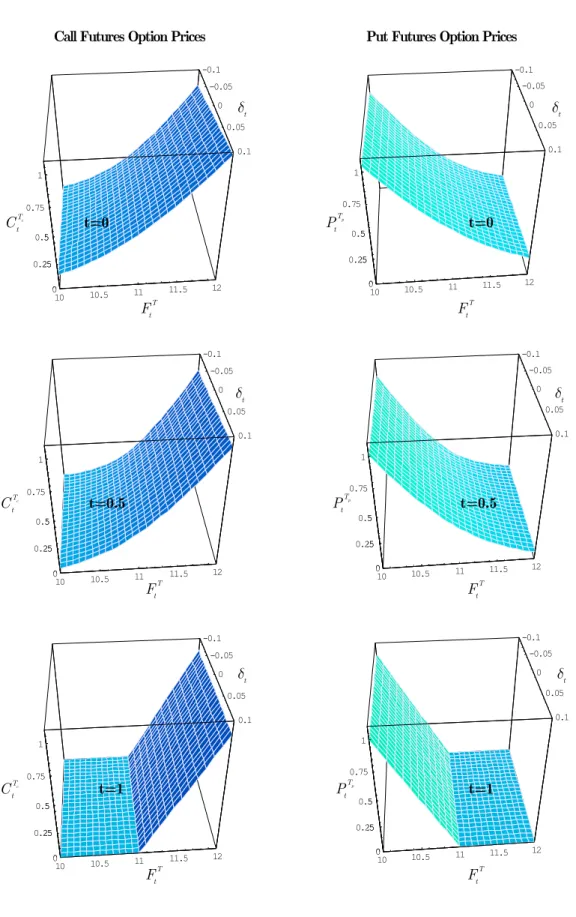
In Chapter 1, we solve the problems imposed in (I). We obtain closed-form solutions for the futures prices. Numerical solutions for the futures options prices are determined by using a method of Fourier transforms. The closed-form solutions for the futures prices are consistent with the theory of storage such that futures prices tend to be lower than spot prices when convenience yields are sufficiently high and vice versa. Moreover, the closed-form solutions lead to the determination of the two state-variables as desired in (II). We achieve (III) by employing a method of maximum likelihood. These works are done in Chapter 2 and Chapter 3. In Chapter 2, we construct a sequence of closed-form approximations of the transition density of the logarithm futures prices process, and hence, the log-likelihood function of futures prices data and prove its convergence in probability to the true log-likelihood function. This convergence implies that the limit of the sequence of approximate maximum likelihood estimators is close to the true maximum likelihood estimators which can be inferred to the true-parameters describing the dynamics of the process. In Chapter 3, we apply model (M) to two agricultural commodities in Thailand, rice and natural rubber. We use the daily futures prices data of the two commodities obtained from the Agricultural Futures Exchange of Thailand (AFET) in two time periods in August 2004 to August 2006.

(14)

Introduction

The estimation results show a clear seasonal pattern in both price and convenience yield volatilities of the two commodities. In addition, the numerical results indicate that the convenience yields tend to be high when the inventory/supply is low, and vice versa. However, there is an impact from the Thai price intervention scheme on the domestic rice prices which can be noticed from the daily extracted rice price volatilities such that they are less variable than the daily extracted rubber price volatilities. Price differences and correlations between the observed and the predicted futures prices are computed for several futures contracts of rice and natural rubber. The results obtained show that the price differences are insignificantly different from zero and the correlations are highly positive. This implies that our model is applicable for the two commodities prices. Furthermore, we observe that, for each selected futures contract, the price differences on the days close to its maturity date are hardly realized by the market participants. In the economic point of view, these results can be explained by the equilibrium in the futures market, namely, the observed futures prices approach their corresponding no-arbitrage futures prices when the futures market is close to the equilibrium. Finally, we investigate the situations known as backwardation and contango in AFET by observing on the forward surfaces for the two commodities in the sample periods. We have found that, for long maturity futures contracts, the futures market of rice exhibited backwardation, while the futures market of natural rubber exhibited contango. These results can be explained as follows. In the long run futures of the two commodities prices, the market has expected a decrease in rice prices, but an increase in natural rubber prices.

The remaining of this dissertation is organized as follows.

In Chapter 1, we briefly review the theory of storage as a motivation to develop a model of commodity prices. Then model (M)is presented in a concrete mathematical way. Sufficient conditions on the convenience yield process are given to ensure that the volatilities are always positive. Milstein scheme is used to simulate sample paths of the two state variables and then Monte Carlo method is employed to evaluate approximate no-arbitrage futures prices. The closed-form no-arbitrage futures prices are derived in both cases, the convenience yields are assumed deterministic and stochastic. Using two no-arbitrage futures prices having different maturities, we derive extraction formulas for the two state-variables. Applying the Itô formula, we write down the dynamics of logarithmic futures prices which are used as the underlying process in estimation of the parameters based on the maximum likelihood approach. The numerical solutions for European futures option prices are derived in the last subsection of the chapter.

(15)

Introduction

In Chapter 2, we solve the forward Kolmogorov equation to obtain the forward transition density of the log-futures prices process. Since the obtained forward transition density contains integral terms of a discretely observed function, we derive a closed-form approximation of the forward transition density by using observed futures prices data and investigate the error estimate. The remaining of the chapter is devoted to a construction of the approximate log-likelihood function of logarithmic futures prices data and the poof of its convergence in probability sense to the true log-likelihood function as previously mentioned.

In Chapter 3, we calibrate model (M) using the daily futures prices data of rice and natural rubber obtained from AFET. We start the chapter by informing the backgrounds in rice and rubber productions and prices in Thailand. Next, we explain more precisely about the futures prices data of rice and rubber in terms of contract specifications and the sample time periods. Using the results obtained from Chapter 1 and Chapter 2, we specify the parameters set and the constraints and then we estimate the model parameters based on the maximum likelihood approach. The optimization problems arising with the use of the estimation method are solved using a heuristic algorithm known as Differential Evolution (DE) provided in Mathematica. The estimation results are reported with discussions focusing on the implications for the prices of rice and natural rubber in Thailand. Using the estimated parameters, we compute the corresponding no-arbitrage (predicted) futures prices. Then we introduce the measurements for price differences and correlations between the observed futures prices and the predicted futures prices. We report the price differences and the correlations of the two commodities via two series of graphs and a discussion about the results obtained is provided thereafter. In the last section of the chapter, we analyze the implications of model (M) for capital budgeting decisions. We display the forward surfaces for the two commodities obtained from model (M)in the sample periods and then a discussion about the situations known as backwardation and contango observed on the forward surfaces is provided therein.

We finally conclude this dissertation with summaries and an outlook of interesting future developments in modeling of commodity prices.

(16)

C

h

a

p

t

e

r

1

S

t

o

c

h

a

s

t

i

c

M

o

d

e

l

i

n

g

f

o

r

C

o

m

o

d

i

t

y

P

r

i

c

e

s

a

n

d

V

a

l

u

a

t

i

o

n

o

f

C

o

m

o

d

i

t

y

D

e

r

i

v

a

t

i

v

e

s

u

n

d

e

r

S

t

o

c

h

a

s

t

i

c

C

o

n

v

e

n

i

e

n

c

e

Y

i

e

l

d

s

a

n

d

S

e

a

s

o

n

a

l

i

t

y

This chapter starts by introducing the conceptual ideas in the theory of storage relating to the stochastic behavior of commodity prices. Then model (M) introduced in Introduction is described in a concrete mathematical way. Sufficient conditions on the convenience yields process are given for the inaccessibility to nonpositive values of the volatilities. Milstein scheme is run for simulating sample paths of the two state variables and Monte Carlo technique is employed to evaluate approximate no-arbitrage futures prices. Furthermore, we derive closed-form solutions for no-arbitrage futures prices in both cases: the convenience yields are assumed deterministic and stochastic. Subsequently, we derive extraction formulas for the two state-variables under the assumption that two no-arbitrage futures prices having different maturities can be observed. Using the Itô formula, we write down the dynamics of logarithmic futures prices which will be used in Chapter 2 as the underlying process in estimation of the model parameters based on a maximum likelihood approach. The remaining of this chapter is devoted to the derivation of the numerical solutions for European futures options prices.

1

.

1

T

h

e

o

r

y

o

f

S

t

o

r

a

g

e

The aim of this section is to briefly review the theory of storage to be a motivation for developing a stochastic model for commodity prices in the next section. The important term “convenience yield” arising from inventories of storable commodities, and the stochastic behaviors of convenience yields are explained and investigated, respectively.

1

.

1

.

1

I

n

v

e

n

t

o

r

i

e

s

a

n

d

C

o

n

v

e

n

i

e

n

c

e

Y

i

e

l

d

s

Consider a competitive commodity market subject to stochastic fluctuations in production and/or consumption. Market participants (producers, consumers, and possibly the third party) will hold inventories. These inventories serve a number of functions. Producers hold them to reduce costs of adjusting production over time, and also to reduce marketing costs by facilitating production and delivery scheduling and avoiding stock outs. Industrial consumers also hold inventories, and for the same reasons – to reduce adjustment costs and

(17)

1.1 Theory of Storage

facilitate production (i.e., when the commodity is used as a production input), and to avoid stock outs. Pindyck (2001) [P-01] explained the function of inventory in a competitive commodity market that it acts as a “lubricant” for both producers and industrial consumers to mitigate the impacts of stochastic fluctuations in production and/or consumption.

In the cash market, purchases and sales of the commodity for immediate delivery occur at a price that we will refer to as the “spot price”. Because inventory holding can change, the spot price does not equate production and consumption. Pindyck (2001) [P-01] characterized the cash market as a relationship between the spot price and “net demand”, i.e., the difference between production and consumption. Let N_t denote the inventory level at time t. The change in inventory level at time t, denoted by %N_t, is given by

%Nt ( ;S zt t,Ft ) ( ;S zt t ,Ft )

S S D D

S D (1.1.1)

where S_t is the spot price at time t, ( ;SS z_t S,FS) is a supply function, ( ;DS z_t D,FD) is a demand function, zS is a vector of supply-shifting variables, zD is a vector of demand-shifting, FSand FD are random shocks such as from unpredictable changes in tastes and/or technologies.

Equation (1.1.1) indicates that the cash market is in equilibrium when net demand equals net supply and then we obtain the following inverse net demand function:

S_t S_t(%N z_t; _tD,z_tS,F F_tD, _tS). (1.1.2) Pindyck (2001) [P-01] concluded that because sS/sS_t 0and sD/sS_t 0, the inverse net demand is upward sloping in %N_t, i.e., a higher price corresponds to a larger S and smallerD, and thus a larger%Nt. He also pointed out that an increase in price volatility implies an increase in the demand for inventory. In other words, price volatility has a negative relationship with inventory level, i.e., an increase in inventory level can reduce price volatility. Other things equal, market participants will want to hold greater inventories in order to buffer these fluctuations in production and consumption. On the relationship between the demand for inventory and commodity price, he concluded that one should be willing to pay more to store a higher-priced good than a lower-priced one. When inventory holdings can change, production in any period need not equal consumption. As a result, the market-clearing price is determined not only by current production and consumption, but also by changes in inventory holdings.

(18)

1.1.1 Inventories and Convenience Yields

The calculation of profitability for holding inventories of the commodity spot rests on the determination of the influence of inventories, production and consumption on the expected spot price. In the commodity literature, supply of storage theory describes this relationship. An excellent summary of these concepts appears in Cootner (1967) [C-01].

The direct costs of holding inventory include warehouse rental and insurance. These costs are thought to be relatively constant over a wide range of inventory levels. Holding inventory ties up capital. An implicit interest charge is usually including in the direct costs of carrying inventory. The difference between futures price and spot price is termed the basis. When the direct costs of carrying inventory are netted out of the basis, there is an empirically substantiated residual component termed the marginal convenience yield. This relationship is depicted in Figure 1.1 (the “supply of storage” curve).

The classic explanation of the marginal convenience yield phenomena is that con-venient inventories provide benefits to the holders of inventory by reducing stock out costs. Also, convenient inventories reduce the chance of turning away good customers (or increase the chance of adding new customers) when inventories are scarce. Thus this theory holds that consumers will pay inventory holders for reducing their costs to locate supplies in times of scarcity. While there has been no completely satisfactory explanation of the supply of storage phenomena, the empirical effect exists for many commodities (e.g., Brennan (1958) [B-04], Working (1949) [W-01]).

Net Convenience yields on a commodity can be thought of in the same way as dividend yields on a common stock. Net convenience yields can be separated into gross convenience yields and costs of carry. Gross convenience yield is the value of all the advantages of possessing the commodity, whereas the cost of carry is the cost of the disadvantages. The net convenience yield is the result of subtracting the cost of carry from the gross convenience yield and it can in many cases be negative. Normally the convenience yield is quoted as a continuously compounded yield (as a continuous compounded interest rate). Under the no-arbitrage assumptions, it is well known that the spot-forward relationship holds for any storable commodity, i.e.,

( )( ) ( ( ))( )

,

T r T t r c c T t t t t

F S e E S e T t, (1.1.3) where FtT is the forward (or futures) price

1

of the commodity on day t maturity at date T,

t

S is the commodity spot price on day t, r is the continuously compounded interest rate,

E is the net convenience yield, c is the gross convenience yield, c is the cost-of-carry yield. These constants are taken over the period from day t to day T.

1

(19)

1.1.1 Inventories and Convenience Yields

US$

Direct Costs of Carrying Inventory

Marginal Convenience Yield at N0

0 N0 Inventory level

Basis = Futures price – Spot price.

Figure 1.1: The “Supply of Storage” curve

We summarize the important implications of the theory of storage as follows.

S1: The volatility of a commodity spot price tends to be inversely related to the level of global stock. In the case of stock outs, spot prices change dramatically in response to supply and demand.

S2: The price of a commodity, its volatility, and the convenience yield, are positively correlated since they are negative related to the inventory level. This feature is called the “inverse leverage effect”, namely, the positive relationship between commodity prices and their volatility.

S3: Convenience yields fluctuate considerably overtime. Some of these fluctuations are predictable, in that they correspond to “seasonal variation” in the demand for storage. Much of the variation in convenience yield, however, is unpredictable, and corresponds to unpredictable temporary fluctuations in demand or supply in the cash market.

S4: Inventory and demand conditions affect the variances of commodity spot prices and the convenience yields. In addition, under the hypothesis that spot return dynamics are strongly related to variations in fundamental supply and demand conditions, the spot return volatility is increasing in the level of convenience yield (see Fama-French (1988) [F-01] and Ng-Pirrong (1994) [N-01]).

(20)

1.1.2 Mean-Reversion and Seasonality in Commodity Prices

1

.

1

.

2

M

e

a

n

-

R

e

v

e

r

s

i

o

n

a

n

d

S

e

a

s

o

n

a

l

i

t

y

i

n

C

o

m

o

d

i

t

y

P

r

i

c

e

s

Mean-Reversion is one of the main properties that has been systematically incorporated in the recent literature on commodity price modeling. Commodity prices neither grow nor decline on average over time, but they fluctuate around their long-run mean. In other words, they tend to mean-revert to a level which may be viewed as the marginal cost of production. This has been evidenced a number of times in literature (see, for instance, Pindyck (2001) [P-01] for energy commodities and Geman-Nguyen (2005) [G-02] for the case of agricultural commodities).

In a nondeterministic setting the resemblance with interest rates and dividends is preserved. Stochastic models of commodity price behavior typically include both stochastic process for the commodity prices and a separate stochastic process for the convenience yields (Gibson-Schwartz (1990) [G-03], Schwartz (1997) [S-01], Richter-Sørensen(2004) [R-01], and Nielsen- Schwartz (2004) [N-02]). Often, a stochastic process for the convenience yields is modeled in the same way as a stochastic process for interest rates such as the Vasicek model or the Cox-Ingersoll-Ross (CIR) model. These models reflect the mean-reversion behavior of convenience yields as previously described in Introduction.

Besides the mean-reversion behavior of commodity prices, the other main empirical characteristic that makes commodities strikingly different from stocks, bonds, and other conventional financial assets, is seasonality in prices (e.g., the discussion in Routledge-Seppi-Spatt (2000) [R-02]). Many commodities, such as agricultural commodities or natural gas, exhibit seasonality in prices, due to harvest cycles in the former case and changing consumption as a result of weather patterns in the latter case. In term structure model of commodity prices, some research has been conducted on the seasonality of commodity prices. Sørensen (2002) [S-02] began with a model describing the dynamics of the (log-) commodity spot price as the sum of a deterministic seasonal component, a non-stationary state-variable, and a stationary state-variable. The deterministic term in seasonal component is modeled by a parameterized linear combination of trigonometric functions with seasonal frequencies. The same type of formalization was introduced by Richter-Sørensen (2004) [R-01] and Geman-Nguyen (2005) [G-02]. The models take the commodity spot price, the instantaneous convenience yield, and the volatility of the convenience yield and the volatility of commodity price as separated state-variables. Nevertheless, those three models do not allow the return volatilities to depend on the level of convenience yield as suggested by the theory of storage.

(21)

1.2.1 The Model

1

1.

.2

2

St

S

to

oc

ch

ha

as

st

ti

ic

c

Mo

M

od

de

el

li

in

ng

g

fo

f

or

r

Co

C

om

mm

mo

od

di

it

ty

y

Pr

P

ri

ic

ce

es

s

Stochastic modeling for commodity prices plays an important role in pricing commodity derivatives such as futures contracts and options, under the no-arbitrage assumptions. Early studies in this area typically assumed that the commodity spot prices and the instantaneous convenience yields are random and they are followed a joining stochastic process with constant correlation. The excellent literature review on stochastic models of commodity spot prices can be found in Lautier (2003) [L-01]. Using those models, one can derive fair-prices of futures or options either in closed-form solutions or numerical solutions. In this section, we present a stochastic model of commodity spot prices based on the theory of storage and seasonality as described in the previous section. Sufficient conditions for the convenience yield process are proposed for having volatilities of the commodity prices to be meaningful. The Mote Carlo Simulation is employed to evaluate the approximate futures prices. Moreover, under deterministic convenience yields, the no-arbitrage futures prices are derived.

1

.

2

.

1

T

h

e

M

o

d

e

l

The model of commodity spot prices developed in this research is an extension of the model proposed by Nielsen-Schwartz (2004) [N-02]. By incorporating seasonality into the model, the commodity spot prices process ( )S_{t t}_{[0, ]}_T and the instantaneous convenience yields process( )E_{t t}_{[0, ]}_T under an equivalent martingale measure satisfy the following stochastic differential equations (SDEs):

2 (1) 1 2 1 2 (2) 1 2 1 2 ( ( )) (1.2.1) ( _T( ) ( )) t t S t t t t t t t t t t dS r S dt S dW d t _E dt _E dW E M C E C C E C E B LE M C E C T C E C ²¦ _¦¦ » ¦ _¦¦¼

with an initial condition (S0,E0),where T 0. In the model, r is the risk free interest rate,

0, 1,2,

i i

C are parameters measuring of the impact of convenience yields on the volatilities of the commodity spot prices. The deterministic seasonal function B_T( )t is of the following form:

(1) (2) 0 1 ( ) ( ) cos(2 ) sin(2 ) , T K k k k t f T t kt kt B B B B B Q B Q _¬

® (1.2.2)

where KBdetermines the number of terms in the summation and B B₀, _k(1),B_k(2),k 1, ...,KB,are constant parameters. The non-specific function ( )f t_B is a positive function determining the magnitude of the periodic terms on the RHS of Equation (1.2.2) at time t.

(22)

1.2.1 The Model

It should be noted that the form of B_T( )t is a flexible and natural choice of modeling the seasonal aspects of commodity price behavior in continuous time which is also applied in Richter-Sorensen (2004) [R-01] with the case that f_B w1. In this research, we choose

2 ( 2) ( ) , p t pt p p p p e f t e B p2 p, (1.2.3)

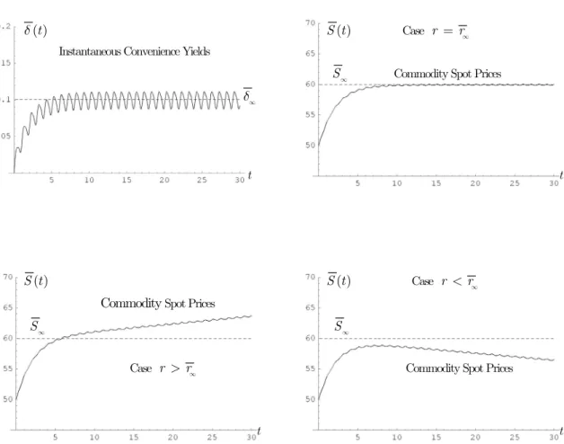
for 0b bt T,where the constants p and p₂ are given in Proposition 5. With this choice of ,f_B B_T( )t still behaves as the case f_B w1 on [0, ]T which can be used to describe the seasonal variation in the convenience yield process3

. Moreover, we are able to derive closed-form solutions for futures prices as expressed in Proposition 5.

The parameter L0 is the magnitude of the speed of the convenience yields mea-suring the degree of reversion to the deterministic seasonal pattern in the convenience yield. The parameter T_E 0 is the magnitude of the impact of convenience yields on volatility of themselves. We let (1) (2)

[0, ]

( t , t )t T

W w W W denote a two-dimensional Brownian motion under the probability space ( ,8 ,)with a filtration(t t)[ 0, ]T.The two Brownian motions are correlated with a constant S ( 1,1),i.e.,

(1) (2)

t t

dW dW Sdt for all t [0, ].T (1.2.4) In our setting, we have assumed that there are no assets that are clearly instantaneously perfectly correlated with the state variables St and Et. In other words, the values of St and

t

E cannot be observed in our setting. Thus, it does not seem possible to construct a hedge portfolio that eliminates all the risk. This causes the risk premium of spot price and the convenience yield risk arise (as proposed by Hull-White (1987) [H-04]) and they are added in the drift terms of the state variables S_t and E_t, respectively. In our model, we assume that the risk premium of the commodity spot prices is proportional to the variance of commodity spot prices and the convenience yield risk is proportional to the variance of instantaneous convenience yield (as suggested by Cox-Ingersoll-Ross (1985) [C-02]). We let M_S and M_E

denote the constants of the proportionalities (see Appendix A).

The model (1.2.1) has two stochastic factors. The first factor is the commodity spot price which follows a Geometric Brownian Motion (GBM) with a time-varying volatility. The second factor is the instantaneous convenience yield which follows an extended CIR process with adding the deterministic seasonal function BT( )t in the drift term of the process.

3

(23)

1.2.1 The Model

The time-varying volatilities of the commodity spot prices and the instantaneous conve-nience yields are proportional to the square root of the instantaneous conveconve-nience yields. The correlation between the commodity spot price process and the instantaneous convenience yield process S is assumed constant. The direct proportionality of the commodity spot price volatilities and the instantaneous convenience yield volatilities to the square root of the instantaneous convenience yields reflect the effect of supply, demand, inventory, and seasonality in the commodity prices and the convenience yield volatilities as suggested by the theory of storage.

In this research, we assume that the risk free interest rate r is known. The 82KB

unknown parameters contained in the vector R defined by

( ) ( )

1 2 0 1 2

: ( , , , _E, _S, _E, , , k, k ),

R C C L T M M S B B B k 1, 2, ...,KB,

will be estimated based on a maximum likelihood approach. Since we cannot observe S_t

and Et from the market under this setting, only futures prices are available in the market.

Hence, we use the logarithmic futures prices process as the underlying process instead of S_t

and E_t to construct a closed-form approximation of the true likelihood function of the logarithmic futures prices data. The closed-from approximation will be used as an objective function for constructing approximate maximum likelihood estimators of the unknown para-meters. These works will be done in Chapter 2 and Chapter 3.

1

.

2

.

2

S

u

f

i

c

i

e

n

t

C

o

n

d

i

t

i

o

n

s

f

o

r

t

h

e

C

o

n

v

e

n

i

e

n

c

e

Y

i

e

l

d

s

P

r

o

c

e

s

In this research, we allow E_t can be either negative or positive or zero because it is the difference between the gross convenience yield c_t and the cost-of-carry yield c_t, i.e.,

,

t ct ct

E _(1.2.5)

for all t [0, ].T However, having the volatilities of S_tand E_tto be meaningful, the following condition must be satisfied:

2

1,

t

C C

E - a.s. for all t [0, ],T (1.2.6) which is equivalent to the condition

1 2

ˆ :_t _t 0,

E C E C - a.s. for all t [0, ].T (1.2.7) The condition (1.2.6) tells that the instantaneous convenience yields must be bounded from below over the time period of consideration. Suppose that c_t w0, the positive ratio C₂ /C₁

(24)

1.2.2 Sufficient Conditions for the Convenience Yields Process

Since the dynamics of ˆE_t is an extension of the CIR model of the form:

(2) 1 1 ˆ ₍ _{( )} ₍ _{) )}ˆ ˆ _, T t t t t dE V t LM C E_E dt T C_E EdW (1.2.8) where V_T( ) :t C B₁ _T( )t LC₂. (1.2.9) Therefore, some conditions on the parameters must be imposed to ensure that nonpositive values are inaccessible to the transformed process (1.2.8), namely, the volatilities of the commodity spot prices and the instantaneous convenience yields must be positive.

Proposition 1.

For given Eˆ₀ 0,a sufficient condition for the inaccessibility of Eˆ_t to nonpositive values is

(1) (2) 1 0 2 1 2 2 1 ( ; ) 1 . 2 K k k k f T B B E C B R B B LC T C _¬ ® p

(1.2.10) Moreover, under this condition, for given 2

1

0 0

( , )S E D:(0,d q) (_CC ,d),there exists a unique strong solution X w( , )S_t E_{t t}_{[0, ]}_T of the SDEs (1.2.1) with X₀ (S₀,E₀)and X never explodes or leaves D before T, - a.s..

We proved Proposition 1 in Appendix B by applying a Comparison Theorem for Solution of Stochastic Differential Equations proposed by Zhiyaun (1984) [Z-01].

1

.

2

.

3

N

o

-

A

r

b

i

t

r

a

g

e

F

u

t

u

r

e

s

P

r

i

c

e

s

a

n

d

M

o

n

t

e

C

a

r

l

o

S

i

m

u

l

a

t

i

o

n

A fundamental implication of asset pricing theory is that, under the no-arbitrage assumptions, the fair-price of a derivative security (futures or option contract) at a current time can be represented by the expected value of its discounted payoff function at the maturity date under a risk-neutral probability measure. In fact, valuing derivatives reduces to computing the expectation with respect to the probability measure. In terms of pricing futures contracts, the following theorem is necessary.

Theorem 1.2.1.

Under the no-arbitrage assumptions in a futures market, the no-arbitrage futures price on day t with maturity date T, denoted by F_tT,must satisfy

| , T t T t F E _¡S ¯_° ¢ ± (1.2.11)

where the expectation is taken under a risk-neutral probability measure conditioned on the information _t.

(25)

1.2.3 No-Arbitrage Futures Prices and Mote Carlo Simulation

Relation (1.2.11) tells that the no-arbitrage futures price today is an unbiased estimator of the spot price at the maturity date of the contract where we consider under the risk-neutral probability measure and the information available today.

To apply the Mote Carlo approach for evaluating the approximate no-arbitrage futures prices, there are three steps as summarized by the following:

(M1)Simulate a sample path of the commodity spot prices by using the model (1.2.1) on the time interval [ , ]t T to obtain S(1)( )T for the first simulation.

(M2)Repeat the procedure (M1) to obtain ( )

( ), 2,..., ,

i

S T i N for a large integer N.

(M3)Construct an estimator S TN( ) of E S[ T] as follows:

( ) 1 1 ( ) : ( ) N i N i S T S T N

_.

Suppose that S( )i( ),T i 1,2,...,N, are independent and identically distributed random sample with mean E S[ _T] and variance T_T2 d.We define the difference between the estimator ( )S T_N and E S[ _T](or the random estimate for the mean error) as follows:

: S T_N( ) E S[ _T].

N

We can decompose the random estimate ˆN into two parts: that is as ˆNNsys Nstat, where :Nsys E[ ]N denotes the systematic error and Nstat denotes the statistical error.

The central limit theorem asserts that, as N l d,Nstat is asymptotically normal distributed

with mean zero and

2 ˆ Var [ ] Var [ ] T . stat N T N N x (1.2.12)

Expression (1.2.12) implies that the standard error ˆN tends to zero with N convergence rate. Hence, in order to obtain sufficiently small confidence intervals it is important to begin with a small variance in the random variable S T_N( ).With a direct simulation method one tries to fix the variance of S TN( ) to a value which close to that of the variance of ST.

However, this variance, which depends on the stochastic differential equations (1.2.1), may sometimes be extremely large. This leads to the problem of variance reduction which is beyond the scope of this research.

To simulate sample paths of commodity spot prices and instantaneous convenience yields, we transform the model (1.2.1) to a diffusion model driving on two independent Brownian motions (1)

W and (2)

.

(26)

1.2.3 No-Arbitrage Futures Prices and Mote Carlo Simulation (1) (2) 1 11 12 (1) (2) 2 21 22 ( , , ) ( , , ) ( , , ) (1.2.13) ( , , , ) ( , , ) ( , , ) t t t t t t t t t t t t t t t t t t dS b t S dt t S dW t S dW d b t S dt t S dW S t dW E T E T E E E T E T E ²¦ _¦¦ » ¦ _¦¦¼ where 1( , t, )t ( t S( 1 t 2)) t b t S E rE M C E C S , 2( , t, )t ( T( ) t ( 1 t 2)) b t S E B t LE M C E_E C , 11( ,t St, )t 1 t 2St T E C E C , T12( ,t St, )Et 0, 21( ,t St, )t E 1 t 2 T E T S C E C , and T₂₂( ,t S_t, )E_t T_E 1S2 C E₁ _t C₂ .

In order to have close pathwise approximations of the Itô processes in (1.2.13), we prefer the Milstein scheme to simulate sample paths of the processes. Under the regular conditions, the Milstein scheme converges with strong order 1.0 (see Kloeden-Platen (1999) [K-02]). First, we shall consider a time discretization ( )t _%_t with

0 1 ... n ... M

t t t t t T (1.2.14) on the time interval [ , ]t T for some integer M, in which the equidistant case has step size

T t t

M

% . (1.2.15)

The following recursive formulas derived by using the Milstein scheme are run for simulating the sample paths:

1 2 1 2 1 2 2 2 ( ) ( ) ( , ) ( ) ( ) ( ) 1 1 1 ( , ) 1 , 1 ( ) ( ) ( ) ( ) 1 ( , , ) ( , , ) _n ( , , ) , i i j n j i i n n n n n j n t j n j j j j j i i i i n n n n n S S b t S E t T t S E W L T t S E I %

%

1 2 1 2 1 2 2 2 ( ) ( ) ( , ) ( ) ( ) ( ) 2 2 2 ( , ) 1 , 1 ( ) ( ) ( ) ( ) 1 ( , , ) ( , , ) _n ( , , ) , i i j n j i i n n n n n j n t j n j j j j j i i i i n n n n b t Sn t t S W L t S I E E E T E T E %

%

( ) ( ) 0 t, 0 t, i i S S E E 0,1,...,n M1, and i 1,2, ...,N, (1.2.16) where ( , ) , 1, 2, n j n t j W

% are increments of the Brownian motion ( , )

n j n t

W which are normal random variables with mean zero and variance %t.The operators L jj, 1,2, are of the following form: 1 2 j j j L S T T E s s s s . (1.2.17)

(27)

1.2.3 No-Arbitrage Futures Prices and Mote Carlo Simulation For j₁ v j₂ with j j₁, ₂ 1,2, 1 1 1 2 1 2 2 1 ( ) ( , ) ( , ) ( , ) , n n n t s n j n j n j j s s t t I dW dW

¨ ¨

(1.2.18)

are multiple Itô stochastic integrals, and for j₁ j₂

1 1 2 2 ( ) ( , ) ( , ) 1 2 n n j n j j t I %W %t . (1.2.19)

We can approximate of the multiple Itô stochastic integral 1 2 ( ) ( , ) n j j I in Equation (1.2.18) by

1 2 1 2 1 2 2 1 ( , ) ( ) ( ) ( ) ( ) ( ) ( ) ( , ) , , 1 2 n p n n n n n n j j j j p j p j j p j I %t Y Y S N Y N Y ¬ ®

1 2 2 2 1 1 ( ) ( ) ( ) ( ) ( ) ( ) , , , , 1 1 2 2 , 2 p n n n n n n j r j j r j r j j r r t r [ Y I [ Y I Q %

(1.2.20) where 2 2 1 1 1 1 , 12 2 p p r r S Q

(1.2.21) and ( ) ( ) ( ) , , , , , n n n j j p j r Y N I and ( ) , n j r

[ are independent standard normal random variables with

( ) 1 ( , ) n n j n j Wt t Y % % _(1.2.22)

forj 1,2, and for some p 1,2,...(see Kloeden-Platen (1999) [K-02]).

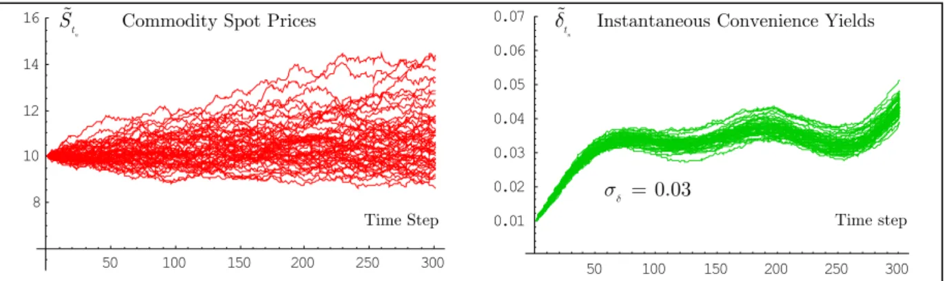
We consider three cases of parameters setting as tabulated in Table 1.1, such that for all cases, the parameters r,C C L S₁, ₂, , ,and B₀are fixed. The number of terms in the summation of the seasonal function KB 2 indicates that there is a possibility to have two local maxima and two local minima in the variation of the seasonal function on the time interval [0, ],T T 1.In Case 2, we increase the volatility of the instantaneous convenience yields from Case 1 by 0.5. In Case 3, we neglect the risk premium of spot prices and the convenience yield risk and increase the magnitude of the seasonal terms. Figures 1.2 – 1.4 show the sample paths of commodity spot prices and instantaneous convenience yields obtained by simulations with the three cases of parameters setting. We do simulations over the time interval [0,1] with the initial values S0 10,E0 0.01, the number of time step

300,

(28)

1.2.3 No-Arbitrage Futures Prices and Mote Carlo Simulation

Table 1.1: Three Cases of Parameters Setting

Parameter Case 1 Case 2 Case 3

r C1 C2 L TE MS ME S K.B 0 B (1 ) (1 ) 1 2 (B ,B ) ( 2 ) ( 2 ) 1 2 (B ,B ) 0.10 0.05 0.01 0.50 0.03 0.05 0.01 0.50 2 0.05 (0.05 , 0.05) (0.02 , 0.02) 0.10 0.05 0.01 0.50 0.05 0.05 0.01 0.50 2 0.05 (0.05 , 0.05) (0.02 , 0.02) 0.10 0.05 0.01 0.50 0.03 0.00 0.00 0.50 2 0.05 (0.10 , 0.10) (0.05 , 0.05)

Next, we evaluate E S[ _T |_t] based on Monte Carlo simulation. In this situation, it is not necessary to have close pathwise approximations of the Itô processes in (1.2.13). In simulating such the sample paths of the processes, it suffices to have a good approximation of the probability distribution of the random variable S_T rather than close approximations of the sample paths. Thus, the type of approximation required here is the weak convergence criterion and we prefer the Euler approximation which converges with weak order 1.0 (see Kloeden-Platen (1999) [K-02]).

By dropping the multiple Itô stochastic integral terms in Equation (1.2.16), the for-mulas become the Euler approximation. We set N 10, 000, the distribution of the com-modity spot prices at t 1, under Case 1 of parameter setting, is illustrated in Figure 1.5. The distribution is right-skewed with mean S_N(1)10.6959S₀.This result implies that, under this case, the market participants expect the higher spot price at t 1 with a high probability. As shown in Figure 1.2, the instantaneous convenience yields are lower than the interest rate. This makes the futures price to be higher than the spot price at t 0.

Overall, the Mote Carlo method proves to be flexible and easy to implement or modify. The method can deal with extremely complicated or high-dimensional problems. Moreover, the current advances in technology have reduced the computation time and have made the method to be more attractive. However, there are several disadvantages to this methodology; very complicated problems may require a very high number of simulations for an acceptable degree of accuracy and this may be