INTERNATIONAL CENTRE FOR ECONOMIC RESEARCH
WORKING PAPER SERIES
Umberto Cherubini, Elisa Luciano
MULTIVARIATE OPTION PRICING WITH COPULAS
Working Paper no. 5/2002 January 2002
APPLIED MATHEMATICS WORKING PAPER SERIES
Multivariate option pricing with copulas
Umberto Cherubini
University of Bologna
and ICER, Turin
Elisa Luciano
University of Torino
and ICER, Turin
¤January 2002
Abstract
In this paper we suggest the adoption of copula functions in order to price multivariate contingent claims. Copulas enable us to imbed the marginal distributions extracted from vertical spreads in the options mar-kets in a multivariate pricing kernel. We prove that such kernel is a cop-ula fucntion, and that its super-replication strategy is represented by the Fréchet bounds. As applications, we provide prices for binary digital op-tions, options on the minimum and options to exchange one asset for an-other. For each of these products, we provide no-arbitrage pricing bounds, as well as the values consistent with independence of the underlying assets. As a …nal reference value, we use a copula function calibrated on historical data.
Keywords: option pricing, basket options, copula functions, non-normal returns.
¤Corresponding Author: Dept. Statistics and Applied Mathematics, P.zza Arbarello 8,
I-10121 Torino, e-mail:[email protected]; the Authors wish to thank participants at the Con-ferences “Managing Credit and Market Risk”, Verona, May 2000, “New Advances in Market and Credit Risk Measurement”, Ascona, June 2000. All remaining errors are ours.
1. Introduction
One of the open issues in contingent claim pricing is the extension of the well-known risk-neutral valuation technique to the multivariate case, that is the case of contingent claims written on “baskets” of several underlying assets, rather than on a single security.
Multivariate contingent claims have been “traditionally” represented by tions on futures, whenever the underlying entails a delivery grade or quality op-tion. Options on the maximum, minimum or options to exchange one asset for another are other “traditional” examples of multivariate claims. Recently, binary digital options have been added to the list. More generally, one can envisage a multivariate feature in every OTC contract, due to the joint riskiness of the underlying and the counterpart business (Klein, 1996).
As the existing literature demonstrates, the pricing problem of multivariate contingent claims is not elementary, whenever the simplifying – and sometimes unrealistic – hypothesis of independence or perfect correlation between the un-derlying risks is abandoned. It becomes even more involved when another ques-tionable assumption is dropped, that of joint normality.
In this paper we abandon both the linear correlation and gaussian assumptions. We explore copula functions as pricing devices. Copulas allow us not only to separate the impact on the joint distribution of the marginals and the association, but also to exploit non-parametric measures of the latter.
The paper is structured as follows: section 2 presents the multivariate pric-ing problem in detail. Section 3 introduces the notion of copula, reviews some of its properties and introduces the relationship with well-known non-parametric association measures. Section 4 explains how to use copulas to represent the mul-tivariate pricing kernel of the economy. Section 5 presents an extensive application to four market indices (Mib30, S&P500, FTSE, DAX), for which we price binary digital options, options on the minimum and options to exchange one asset for another. Section 6 concludes.
2. Multivariate Contingent Claims
In mathematical terms, the multivariate feature of a contingent claim shows up in a pay-o¤, which in general can be written as
where g(:) is a univariate pay-o¤ function which identi…es the derivative con-tract, f(:) is a multivariate function which describes how the n underlying secu-rities determine the …nal cash-‡ow, Si denotes the price of thei¡th underlying
security and T is the contract maturity. In what follows, for notational conve-nience, we skip the reference to T whenever it is not needed.
As an example, in the case of rainbow call options g is the familiar payo¤ function
g(f) = max(f ¡K;0)
where K is the strike price, while f(¢) may select the minimum (or maximum or some kind of average) of nassets:
f(Si(T); T;i= 1;2:::n) = min (Si(T);i= 1;2:::n)
The option on the minimum (or maximum) was …rst studied by Stulz (1982) in the lognormal case. In the same setting, Margrabe (1978) had already studied the most speci…c instance of the option to exchange.
Another example, which is easier to address, is the multivariate digital option. In this case the g function is simply a multiplicative constant; f spots the event that each underlying is greater than or equal to some corresponding threshold Ki
f(Si(T); T;i= 1;2:::n) =If(S1(T)¸K1)\::\(Sn(T)¸Kn)g
where I is the indicator function.
The multi-asset feature has a long standing history in fairly standard and mature derivative markets. The most standard case is o¤ered by the market of options on futures: as typically the standardization feature of futures contracts entails a delivery grade option (or quality option), the option on the futures contract may be seen as an option written on a basket of deliverable products. The quality option issue, however, has not posed much of a problem as for the pricing techniques: in fact, the standardization feature of futures contracts also implies that most of the products eligible for delivery were chosen in such a way as to grant a high degree of similarity. In other words, the products chosen as deliverable under the contract are typically strongly correlated and considering them perfectly correlated is not much of a mistake. This is what is done when using a one factor model of the term structure in order to evaluate the quality option on long term interest futures and options .
It cannot be ignored that the perfect correlation assumption always leads to an approximation of the problem. Even in the case of the quality option in
interest rate futures we know that this approach is not able to take into account some market anomalies, such as coupon or seasoning e¤ects, that may play a relevant role in the determination of the cheapest asset to deliver. Besides this, there are also cases in which the imperfect correlation issue cannot be avoided, as it represents the main motivation which inspires the product. In fact, the pricing task gets more involved for products in which the multiasset feature is meant to provide diversi…cation. The most straightforward example is o¤ered by call options written on the minimum or maximum among some market indices. In these cases, ignoring imperfect dependence among the markets may lead to substantial mispricing of the products, as well as to inaccurate hedging policies and unreliable risk evaluations.
While the multiasset pricing problem may be already complex in a standard gaussian world, the evaluation task is compounded by the well known evidence of departures from normality. Following the stock market crash in October 1987, departures from normality have shown up in the well known e¤ects of smile and term structure of volatility and have become common ground of work of academics and traders.
Of course, jointly taking into account non-normality of yields and their depen-dence structure makes the two problems far more involved. As a simple example of this complexity, just consider the fact that the standard linear correlation …g-ure that we use to meas…g-ure dependency cannot be safely used in a non-normal world, as it may not be able to take values in the whole range between -1 and +1: the e¤ect is that in a non-gaussian world we may well observe a correlation …gure lower than 1 in a case in which there is perfect dependence between the variables. So, the correlation …gure may lead to mis-representation of the degree of diversi…cation in a portfolio. By the same token, in a non-gaussian world a trader may pursue the task of modifying the correlation …gure of his portfolio to a value which is simply impossible to reach under the real multivariate distribution in the data.
A possible strategy to address the problem of dependency under non-normality is to separate the two issues, i.e. working with non-gaussian marginal probability distributions and using some technique to combine these distributions in a multi-variate setting. This is the approach followed by Rosenberg (1999), who uses the set of Plackett distributions to price bivariate contingent claims consistently with given marginals. In the sequel we generalize his approach using copula functions, of which the Plackett family is only a speci…c case. The main advantage of the copula approach to pricing is to write the multivariate pricing kernel as a function
of univariate pricing functions. This enables us to carry out sensitivity analysis with respect to the dependence structure of the underlying assets, separately from that on univariate prices.
3. Mathematical background
In what follows we give the de…nition of copula function and some of its basic properties, while we refer the reader interested in a more detailed treatment to Nelsen (1999) and Joe (1997). Here we stick to the bivariate case: nonetheless, all the results carry over to the general multivariate setting.
De…nition 3.1. A two-dimensional copula C is a real function de…ned on I2 =d [0;1]£[0;1], with rangeI = [0d ;1], such that
for every (v; z) of I2; C(v;0) = 0 =C(0; z); C(v;1) =v; C(1; z) = z;
for every rectangle [v1; v2] £ [z1; z2] in I2,with v1 · v2 and z1 · z2, C(v2; z2)¡
C(v2; z1)¡C(v1; z2) +C(v1; z1)¸0
As such, it can represent the joint distribution function of two standard uni-form random variables U1; U2:
C(u1; u2) = Pr(U1 ·u1; U2 ·u2)
We can use this feature in order to re-write via copulas the joint distribution function of two (even non-uniform) random variables. The most interesting fact about copulas in this sense is Sklar’s theorem:
Theorem 3.2 (Sklar (1959)). LetF(x; y)be a joint distribution function with continuous marginals F1(x) and F2(y). Then there exists a unique copula such
that
F(x; y) =C(F1(x); F2(y)) (3.1)
Conversely, if C is a copula andF1(x), F2(y) are continuous univariate
distribu-tions, F(x; y) = C(F1(x); F2(y)) is a joint distribution function with marginals
F1(x),F2(y).
The theorem suggests then to represent the multiplicity of joint distributions consistent with given marginals through copulas.
Three speci…c copulas are worth mentioning: theproduct copula, theminimum
copulas are called comprehensive. As for the …rst, the copula representation of a distribution F degenerates into the so-called product copula, C(v; z) = v¢z, if and only if X and Y are independent. As for the others, they derive from the well-known Fréchet-Hoe¤ding result in probability theory, stating that every joint distribution function is constrained between the bounds
max(F1(x) +F2(y)¡1;0)· F(x; y)·min(F1(x); F2(y)) (3.2)
As a consequence of Sklar’s theorem, the Fréchet-Hoe¤ding bounds exist for cop-ulas too:
max(v+z¡1;0)·C(v; z)·min(v; z)
In correspondence of the extreme copula bounds, there is perfect positive and negative dependence between the variables, and every variable can be obtained as a deterministic function of the other (see Embrechts, McNeil and Straumann,1999 for a proof). We can state that
Theorem 3.3 (Hoe¤ding (1940), Frechet (1957)). If the continuous random variables X and Y have the copula min(v; z), then there exists a monotonically
increasing function U such that
Y =U(X) U =F2¡1(F1)
whereF2¡1is the generalized inverse ofF2. If instead they have the copulamax(v+
z¡1;0), then there exists a monotonically decreasing function Lsuch that
Y =L(X) L=F2¡1(1¡F1)
The converse of the previous results holds too.
In the …rst case, X and Y are called comonotonic, while in the second they are deemed countermonotonic.
Copulas are linked to non-parametric association measures by useful relation-ships. As an example, Kendall’s ¿ may be proved to be
¿ = 4
Z Z
I2
C(v; z)dC(v; z)¡1 while Spearman’s ½ measure is given by
½= 12
Z Z
I2
C(v; z)dvdz¡3 (3.3) As a consequence of these results, it can be proved that the bounds of¿ and½
are always -1 and +1, while this is not true for the linear correlation coe¢cient, whose value depends on the speci…c shape of the marginal distribution functions, as can be glanced from the relationship
cov(X; Y) =
Z Z
D
(F(x; y)¡F1(x)F2(y))dxdy (3.4)
where D is the cartesian product of X andY’s domains.
A particular class of copulas, so-called Archimedean, is particularly easy to handle and will be used in this paper (see Genest and MacKay, 1986, Genest and Rivest, 1993).
Archimedean copulas may be constructed using a generating fuynction Á : [0;1] ! [0;1] continuous, strictly decreasing, convex and such that Á(1) = 0. Given such a function Á a copula may be generated computing
C(v; z) =Á[¡1] (Á(v) +Á(z)) (3.5) where Á[¡1] is the pseudo-inverse ofÁ:
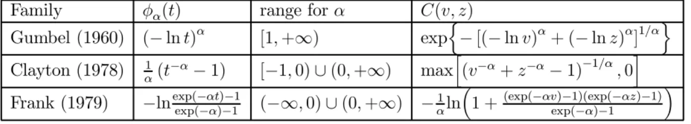
Among Archimedean copulas, we are going to consider only the one-parameter ones, which are constructed using a generator'®(t), indexed by the parameter®.
The table below describes well known Archimedean copulas and their generators (for a complete list see Nelsen, 1999):
Family Á®(t) range for® C(v; z)
Gumbel (1960) (¡lnt)® [1;+1) expn¡[(¡lnv)®+ (¡lnz)®]1=®o Clayton (1978) ®1 (t¡®¡1) [¡1;0)[(0;+1) maxh(v¡®+z¡®¡1)¡1=®;0i Frank (1979) ¡lnexp(exp(¡¡®t®))¡¡11 (¡1;0)[(0;+1) ¡1®ln³1 + (exp(¡®vexp()¡1)(exp(¡®)¡1¡®z)¡1)´
Table 3: some Archimedean copulas
The second and third are particularly interesting since their arecomprehensive
according to the de…nition above. The Gumbel family gives the product copula if
® = 1 and the upper Fréchet boundmin(v; z)for ® !+1: it describes positive association only. The Clayton family gives the product copula if®!0, the lower
Fréchet bound max(v+z¡1;0) when ® =¡1, and min(v; z) for ® ! +1. To end up with, the Frank’s family, which is discussed at length in Genest (1987), reduces to the product copula if ®!0, and reaches the lower and upper Fréchet bounds for ® ! ¡1and® !+1, respectively.
4. Pricing multivariate contingent claims
As a …rst step to price multivariate contingent claims with copulas we may focus on the case of digital binary options. Every practitioner would agree that this case is not simply of an academic interest, as this kind of derivative is present in some widely known structured …nance products such as digital binary notes, that is debt instruments promising to pay a …xed coupon if the prices of two assets are above some prede…ned strike levels at some future date and zero otherwise. In order to price and hedge products like these one has to …nd a replicating strategy for the digital binary option. As there is not a market for them, this task would lead us straight into the problem of market incompleteness. One could even argue that the problem is further complicated by the fact that replicating a digital note written on a single underlying asset would also be involved, as a market of digital options is not available for each and every strike: while this is true, we may assume that products like these may be satisfactorily approximated using vertical spreads, as suggested in the seminal work by Breeden and Litzenberger (1978) and in all the more recent literature drawing from that idea (Shimko 1993, Rubinstein 1994, Derman and Kani 1994a,b to quote a few).
In order to focus on the multivariate feature of the pricing problem, we as-sume that we may replicate and price two single digital options with the same exercise date T written on the underlying markets S1 and S2 for strikes K1 and
K2 respectively. Our problem is then to use these products to replicate a double
binary option which pays 1 if X1 ¸ K1 and X2 ¸ K2 and zero otherwise. Let
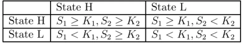
us …rst break the sample space, which coincides with the positive hortant, in the four relevant regions
State H State L
State H S1 ¸K1; S2 ¸K2 S1 ¸K1; S2 < K2
State L S1 < K1; S2 ¸K2 S1 < K1; S2 < K2
Table 1: breaking down the sample space for the digital option.
The binary digital option pays 1 unit only if both of the assets are in state H, that is in the upper left cell of the table. The single digital options written
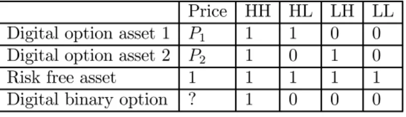
on assets 1 and 2 pay in the …rst row and the …rst column respectively. In table 2 below we sum up the payo¤s of these di¤erent assets and we make clear which prices are observed in the market. We assume that the risk free rate be zero and we denote with P1; P2 the prices of the single digital options
Price HH HL LH LL Digital option asset 1 P1 1 1 0 0
Digital option asset 2 P2 1 0 1 0
Risk free asset 1 1 1 1 1 Digital binary option ? 1 0 0 0 Table 2: Prices and payo¤s for digital options
Our problem is to use no-arbitrage arguments to recover the price of the binary digital option. Some interesting no arbitrage implications can be easily obtained by comparing its pay-o¤ with that of portfolios of the single digital options and the risk free asset. Furthermore, as we face a pricing problem in an incomplete market, we may expect to …nd super-replication strategies leading to pricing bounds for the binary asset. The following proposition states such bounds for the price.
Proposition 4.1. The no-arbitrage price P(S1 ¸ K1; S2 ¸ K2) of a digital
bi-nary option is bounded by the inequality
max(P1+P2¡1;0)·P(S1 ¸K1; S2 ¸K2)·min(P1; P2) (4.1)
Proof: assume …rst that the right side of the inequality is violated: say that, without loss of generality, it is P(S1 ¸ K1; S2 ¸ K2) > P1; in this case selling
the binary digital option and buying the single digital option would allow a free lunch in the state [S1 ¸ K1; S2 < K2]. As for the left side of the inequality, it
is straightforward to see that P must be non-negative. There is also a bound
P1+P2¡1: assume in fact thatP1+P2¡1> P(S1 ¸K1; S2 ¸K2); in this case
buying the binary digital option and a risk-free asset and selling the two single digital options would allow a free lunch in the state [S1 < K1; S2 < K2]¤.
The proposition exploits a static super-replication strategy for the binary dig-ital option: the lower and upper bounds have a direct …nancial meaning, as they describe the pricing bounds for long and short positions in the double binary options. We may take one step further and investigate the features of a pricing function P(S1 ¸ K1; S2 ¸ K2) = C(P1; P2). It may be easily checked that the
Proposition 4.2. The no-arbitrage pricing functionC(v; z)ful…lls the following requirements:
² it is de…ned inI2 = [0;1]
£[0;1]and takes values in I = [0;1];
² for every v and z of I2; C(v;0) = 0 =C(0; z); C(v;1) = v; C(1; z) =z;
² for every rectangle [v1; v2]£ [z1; z2] inI2,with v1 ·v2 andz1 ·z2,
C(v2; z2)¡C(v2; z1)¡C(v1; z2) +C(v1; z1)¸0
Proof: The …rst condition, that the price of the single digital options and that of the digital binary option should be constrained in the unit interval, is trivial, and is the standard no-arbitrage condition that applies to Arrow-Debreu prices. As for the second condition, it follows directly from the no-arbitrage inequality (4.1), by substituting the values 0 and 1 for v = P1 or z = P2. As for the last
requirement, consider taking two di¤erent strike prices K11 > K12 for the …rst
security, and K21 > K22 for the second. Denote with v1 the price of the …rst
digital corresponding to the strike K11; with v2 that of the …rst digital for the
strike K12 and use an analogous notation for the second security. Then, the third
condition above can be re-written as
P(S1 ¸K12; S2 ¸K22)¡P(S1 ¸K12; S2 ¸K21)+
¡P(S1 ¸K11; S2 ¸K22) +P(S1 ¸K11; S2 ¸K21)¸0
As such, it implies that a spread position in binary options paying one unit if the two underlying assets end in the region [K12; K11] £ [K22; K21] cannot have
negative value1¤.
Matching the two propositions above with the mathematical de…nitions given in the previous paragraph we may restate the main results of our analysis as
Proposition 4.3. The arbitrage-free pricing kernel of a multivariate contingent claim is a copula function and the corresponding super-replication strategies are represented by the Fréchet bounds.
1This property is akin to the requirement, in the one dimensional pricing problem, that the
It must be stressed that in order to prove the result we did not rely on any assumption concerning the probabilistic nature of the arguments of the pricing function: these are only required to be no-arbitrage prices of single digital options. In this respect, the may also be viewed as capacities, i.e. non-additive functionals, rather than probability measures, and this enables us to extend the analysis to the presence of frictions or to the case in which the market for options written on any single underlying asset is incomplete. In the case in which the market for single digital options is complete, so that these options can be exactly replicated and the prices are the risk-neutral probabilities
P1 = Pr (S1 ¸K1); P2 = Pr (S2 ¸K2)
we are allowed to give a probabilistic interpretation of the price of a digital binary option, resorting directly to Sklar’s theorem.
First, the price is a function taking as arguments the two single digital options prices: a crucial result is that the restrictions which rule out arbitrage opportuni-ties are the same that de…ne a copula function in multivariate statistics. Second, as the arguments of such function are digital options prices, the risk neutral val-uation principle implies that also the price of the multivariate contingent claim is a distribution function under the risk-neutral probability measure:
C(P1; P2) = Pr(S1 ¸K1; S2 ¸K2) (4.2)
Finally, Sklar’s theorem implies, not surprisingly, that the prices of digital binary options are multivariate distribution functions, as well as the price of univariate digital options represents the corresponding marginal.
The strength of these results is that they enable us to break the multivariate pricing kernel of the economy into a function of marginal univariate kernels: we may then extract separately marginal pricing kernels from vertical spreads and the multivariate pricing kernel of the economy from the dependence structure in the data.
It may be easily checked that the two no-arbitrage bounds in (4.1), which we interpreted as the buyer and seller’s prices, represent the …nancial application of the minimal and maximal copulas of the Fréchet-Hoe¤ding inequality. The …nancial meaning of the two bounds becomes even more relevant if we exploit the result in theorem 3.3, that associates the lower and upper bounds to the case of perfect negative and positive dependence between the two underlying assets. Intuitively, this means that the value of any of the two assets can be recovered
exactly once the value of the other is known. This result is particularly useful since it enables us to reduce the multivariate pricing problem to a standard univariate problem, at least as far as super-replication strategies are concerned, and can be usefully exploited to recover pricing bounds for any bivariate derivative contract. If we now have to recover the pricing bounds of a generic bivariate derivative contract with payo¤ g(f(S1; S2))we may obtain
Proposition 4.4. If two underlying assetsSi; i= 1;2have marginal pricing
ker-nels Pi; i = 1;2 and g(f(S1; S2)) denotes the payo¤ of a bivariate derivative
con-tract whose price is G(S1; S2) we must have
E[gl(S1)]·G(S1; S2)·E[gu(S1)] where gl(S1) d =g¡f¡S1; P2¡1(1¡P1(S1)) ¢¢ gu(S1) d =g¡f¡S1; P2¡1(P1(S1)) ¢¢
and the expectation is computed under the probability measure P1
The evaluation of the two pricing bounds typically would require numerical integration. The numerical evaluation of the pricing bounds could exploit the algorithm used in Cherubini and Esposito (1995): if for example we would like to …nd the upper bound we could partition the domain of S1using the …xed points
of the functionP2¡1(P1(S1))and integrate the relevant pay-o¤ over each interval.
An interesting question is how wide is the range between the two pricing bounds. It may be the case that assuming perfect dependence leads us to overlook the most relevant feature of a multivariate contingent claim. In this case, relying on some …gure representing the dependence structure in the data may help to yield a more precise evaluation of the contingent claim. Indeed, knowing the dependence structure in the data may help to characterize the copula function used in order to price the multivariate contingent claim, as we are going to show in the next sections.
5. Empirical applications
In this section we apply copulas to the pricing problem of multivariate derivatives written on four indices: MIB30, S&P500, FTSE, DAX.
We …rst derive the risk-neutral marginal density function of each index, using the technique of Shimko (1993)2. We then obtain the lower and upper Fréchet
bounds for their joint distribution functions, which are the pricing kernel bounds. In order to pick out a single value between these bounds, one would need to observe at least one price of a multivariate claim. Since typically these products are not traded on organized markets, we present a sensitivity analysis of the multivariate option values with respect to the dependence structure of the underlying assets. As a reference case, we choose a price consistent with the dependence statistics estimated on historical data using a non parametric procedure.
5.1. Descriptive statistics and implied marginal densities
The data used for implied volatilities, time to maturity, dividend points and risk-free rate were downloaded from Bloomberg on March 27, 2000 and refer to Eu-ropean calls closing prices with June expiration and di¤erent strikes. As for the non-parametric dependence estimation, we used the time series of the correspond-ing indices, from January 2, 1999 to March 27, 2000.
We estimate the risk-neutral marginal distribution of each index (MIB30, S&P500, FTSE, DAX) on the cross section data on European calls. As a re-sult, given a quadratic smile function ¾(K) =A0+A1K+A2K2, whereK is the
strike price, we recover the risk-neutral distribution functionFS of the underlying
S: FS(s) = 1 +sn(D2(s)) p T ¡t(A1+ 2A2s)¡N(D2(s)) (5.1) D2(s) = lnsB(XT¡t) ¾(s)pT ¡t ¡ 1 2¾(s) p T ¡t
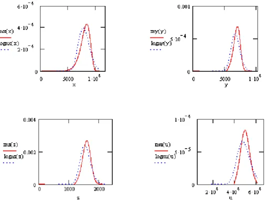
whereT ¡t is the time to maturity,n(¢)andN(¢)are respectively the density and the distribution of the standard normal, X is the current value of the under-lying, less the discounted dividends, and B(T ¡t) is the risk-free discount factor for the same maturity of the option. Figure 6.1. reports the marginal risk-neutral density functions obtained from the data.
Insert here …gure 6.1
2The estimation technique for the marginals can be changed without modifying the core of
Using the four marginals so obtained and (3.4), we numerically compute the lower and upper Fréchet bounds for the joint distributions. Substituting them in (3.3) we recover the correlation bounds in …gure 6.2 below.
Insert here …gure 6.2
The Fréchet bounds could be exploited for super-replication pricing of mul-tivariate claims. Before doing that, we present the results of copula estimation using historical data, that will serve as a reference point for pricing: the copula estimation procedure is described in Frees and Valdez (1998) and based on Genest and Rivest (1993).
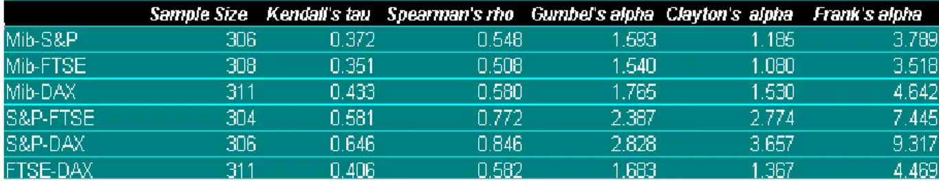
In …gure 6.3 we report the estimated parameters®for the families of Archimedean copulas described in table 3, as well as the standard non parametric statistics (Kendall’s ¿ and Spearman’s½).
Insert here …gure 6.3
In what follows we will use Frank’s copula, both on the ground that it turned out to provide a better …t in all cases - as measured visually and by the mean square error - than the Clayton, and on the fact that the Gumbel copula does not allow for negative dependence.
5.2. Option pricing
Using the Frank’s copula and the estimation of the marginal densities described above we get the following joint distribution for each couple of indices
F(s1; s2) =¡ 1 ®ln µ 1 + (exp (¡®FS1(s1))¡1) (exp (¡®FS2(s2))¡1) exp (¡®)¡1 ¶ (5.2) where FS1(s1); FS2(s2) are de…ned according to ( 5.1). This is the basic tool
for option pricing, once the proper parameter estimates are plugged in. As an example, in …gure 6.4. below we present the joint distribution for the DAX/FTSE case (5.2), together with its level curves3. The distribution was computed using the historical estimate of ®:
Insert here …gure 6.4
3Level curves can be de…ned in terms of risk-neutral joint distributions or in terms of copulas.
With respect to the latter they are de…ned as usual as
©
5.2.1. Digital binary option
First of all, using the joint distribution (5.2) we are able to price digital binary options. In order to stress the immediate relationship between copulas and digital binary prices, we assume a zero interest rate and use proposition 4.3. above. In order to take into consideration a deterministic, non-zero assumption on interest rates, it would be su¢cient to scale the prices presented below with the dicount factor B(T ¡t).
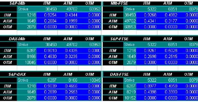
Figure 6.5. below presents some examples, again with ® estimated from his-torical data, for the cases in which the corresponding single digital options are out-of-the-money (OTM), nearly at-the money (ATM) and in-the money (ITM). The digital binary options in the …gure are then evaluated under di¤erent money-ness combinations for each underlying. The maturity is that of the corresponding marginals, i.e. three months.
Incidentally, the reader can easily notice that the familiar behavior of prices with respect to moneyness is respected: prices are decreasing, for every couple of indices, from top left towards bottom right and, ceteris paribus, from left to right and from top to bottom.
Insert here …gure 6.5
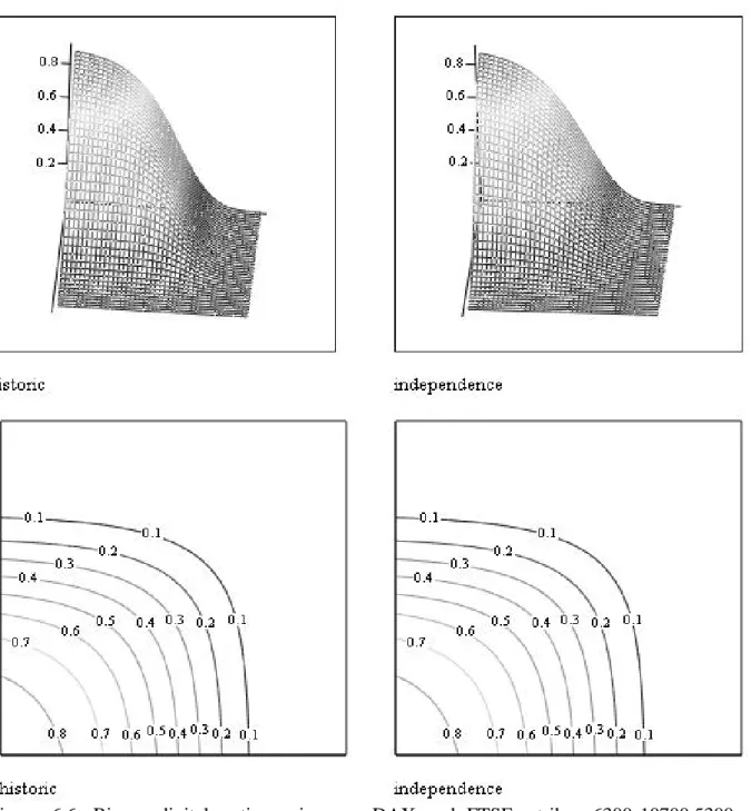
By letting the strikes vary on a …ner grid, we obtain the whole pricing surface for the three-month digital option on DAX and FTSE, which corresponds to the risk-neutral probability that both underlying assets be above the corresponding strikes. In …gure 6.6 below we present the pricing surface corresponding to the historically calibrated copula and to the product copula.
Insert here …gure 6.6
In …gure 6.7 we present a numerical example of the sensitivity analysis shown graphically above. The example refers to the case in which both of the strikes are either ITM or nearly ATM. We analyze how the value of the option changes with respect to the parameter®, as we move from perfect dependence to independence
In the Archimedean case they become
of the underlying assets. By letting ® reach its bounds the binary digital option prices converge to the Fréchet bounds, while the independence case (® = 0) is simply the product copula.
Insert here …gure 6.7
5.2.2. Option on the minimum of two assets
We turn now to the pricing of the option on the minimum between two risky assets, which has been priced, in the Black-Scholes (lognormal) framework, by Stulz (1982). We assume deterministic, non zero interest rates.
The payo¤ of the call option on the minimum, with maturity T, is max(min(S1(T); S2(T))¡K;0)
where K is the strike price. Provided only that interest rates are non-stochastic, its price is B(T ¡t) ·Z +1 K qg(q)dq¡K(1¡G(K)) ¸ (5.3) where g(q) is the risk-neutral density of the minimum, while G(K) is the corre-sponding distribution function evaluated atK. In turn, sinceGcan be computed to be
G(q) =FS1(q) +FS2(q)¡c(FS1(q); FS2(q))
where cis the copula density, the density g(q) is
g(q) =fS1(q) +fS2(q)¡c1(FS1(q); FS2(q))fS1(q)¡c2(FS1(q); FS2(q))fS2(q)
wherec1 andc2 are the partial derivatives ofcwith respect to its arguments, while
fSi, i = 1;2, are the densities corresponding to FSi. These densities turn out to
be fSi(q) =n(D2i(q)) h D2i(q)¡(A1i+ 2A2iq) p T ¡t(1¡D2i(q)D2i(q))¡2A2iq p T ¡ti (5.4) where D2i(q) = ¡ 1 q¾i(q) p T ¡t ¡ D1i(q)(A1i+ 2A2iq) ¾i(q) D1i(q) =D2i(q) +¾i(q) p T ¡t
and the functions D2i(q)and ¾i(q) are de…ned as in section 5.1.
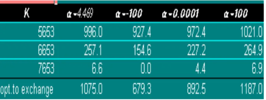
Figure 6.8 presents the prices for ITM, ATM, OTM three-months call options on the minimum between DAX and FTSE, computed according to (5.3) and using our estimate for the risk-neutral joint distribution function.
Insert here …gure 6.8
In the …rst column we present the strike prices, corresponding to ITM (5653), ATM (6653) and OTM (7653) options. Moneyness is de…ned with respect to the FTSE index, whose current value on March 27, 2000, was 6653. From left to right, we present the prices corresponding to the historical association between the two indices (® = 4:469), to an hypothetical quasi perfect positive association (®= 100), to independency (® =:0001) and to quasi perfect negative association (® = ¡100). The reader can easily notice that, ceteris paribus, option prices are increasing with the association between the underlying assets, as the prices get closer to the super-replication values. They are decreasing with the strike, as usual.
5.2.3. Option to exchange one asset for another
The last line of the table in …gure 6.8 presents the price of the option to exchange DAX for FTSE, corresponding to di¤erent ® values. In order to understand the pricing technique used, let us recall that the price of the option to exchange one asset for another, originally derived – for lognormal distributions – by Margrabe (1978), can be obtained as a portfolio of one underlying and a zero-strike option on the minimum. In fact, the payo¤ of the exchange option is
max(S1(T)¡S2(T);0)
which can be rewritten as
S1¡max(min(S1; S2);0)
Recalling that the risk-neutral expected value of the underlying at maturity is the forward price, it follows that its price is the current value of the …rst underlying minus the price of the option on the minimum, with strike equal to zero. Using this device, under the assumption of deterministic, non zero interest rates, we obtain the exchange option value as
S1(t)¡B(T ¡t)
Z +1
0
qg(q)dq
6. Conclusions
In this paper we suggest a strategy to address the joint issues of non-normality of returns and dependence in the multivariate contingent pricing problem. It is well known that under non-normality of returns the linear correlation is not an useful indicator of dependence, as it is not bounded in the unit range. We suggest to resort to the concept of copula in order to account for this problem: using copula functions enables to “decouple” the pricing problem, addressing the speci…cation of marginal distributions and the dependence problem separately. A relevant advantage of this approach is that it is directly amenable to concrete applications: as a matter of fact, we have very well developed markets for many products, and the marginal distributions can be directly computed from the prices of vertical spreads of plain vanilla options. The use of copula functions enables us to link these marginal distributions in a multivariate pricing kernel.
As an example of the power of the approach, we present an application to four stock market indices: for each market we use vertical spreads and the in-terpolation technique due to Shimko to recover the implied marginal probability distributions from the market. We provide prices for a set of multivariate con-tingent claims, such as binary digital options, which represent the basis of prices for all of the bivariate contingent claims in the economy, options on the minimum and options to exchange one asset for another. For each of these products, we provide super-replication prices, as well as the values consistent with indepen-dence of the underlying assets. As a …nal reference value, we show how to price the multivariate options using a copula function calibrated on historical data.
Figure 6.1: Solid lines: risk-neutral densities of DAX (x), FTSE (y), S&P500 (z), MIB30 (u), computed according to (5.4). Dotted lines: corresponding lognormal densities.
Figure 6.3: Estimated Kendall’s ¿, Spearman’s R, and ® for MIB30, S&P500, FTSE, DAX,1/2/99-3/27/00
Figure 6.6: Binary digital option prices on DAX and FTSE, strikes 6300-10700,5300 9300,computed with: the historically calibrated copula and the product one (indipendence).
Figure 6.8: Prices of the call option on the minimum and option to exchange DAX for FTSE
References
[1] Breeden, D.T. and Litzenberger, R.H., 1978, Prices of State-Contingent Claims Implicit in Option Prices,Journal of Business, 51, 621-51.
[2] Cherubini, U. and Esposito, M., 1995, Options in and on interest rate futures contracts: results from martingale pricing theory,Applied Mathematical Fi-nance, 2, 1-16.
[3] Derman, E. and Kani, I., 1994a, The volatility Smile and its Implied Tree, Quantitative Strategies Publication, Goldman-Sachs.
[4] Derman, E. and Kani, I., 1994b, Riding on a smile, Risk, 7, 32-39.
[5] Embrechts, P., McNeil, A. and Straumann, D., 1999, Correlation and depen-dence in risk management: properties and pitfalls, ETHZ working paper. [6] Fréchet, M., 1957, Les tableaux de corrélations dont les marges sont données,
Annales de l’Université de Lyon, Sciences Mathématiques at Astronomie, Série A, 4, 13-31.
[7] Frees, E.,W. and Valdez, E., 1998, Understanding relationships using copulas,
North American Actuarial Journal, 2, 1-25.
[8] Genest, C., 1987, Frank’s family of bivariate distributions, Biometrika, 74, 549-555.
[9] Genest, C. and MacKay, J., 1986, The joy of copulas: bivariate distributions with uniform marginals,The American Statistician, 40, 280-283.
[10] Genest, C. and Rivest, L.P., 1993, Statistical inference procedures for bivari-ate Archimedian copulas, Journal of Amer. Statist. Assoc., 88, 423, 1034-1043.
[11] Hoe¤ding, W., 1940, Massstabinvariante Korrelationstheorie, Schriften des Mathematischen Seminars und des Instituts fur Angewandte Mathematik der Universitat Berlin, 5, 181-233.
[12] Joe, H., 1997, Multivariate models and dependence concepts, Chapman and Hall, London.
[13] Klein, P., 1996, Pricing Black-Scholes options with correlated credit risk,
Journal of Banking and Finance,20, 1211-1230.
[14] Margrabe, W., 1978, The value of an option to exchange one asset for another,
Journal of Finance, 33, 177-186.
[15] Nelsen, R.B., 1999, An introduction to copulas, Springer, New York.
[16] Rosenberg, J.V., 1999, Semiparametric pricing of multivariate contingent claims, NYU- Stern School of Business Working Paper.
[17] Rubinstein, M., 1994, Implied Binomial Trees, Journal of Finance, 49, 771-818.
[18] Shimko, D.C., 1993, Bounds of probability, Risk, 6, 33-37.
[19] Sklar, A., 1959, Fonctions de repartition à n dimensions et leurs marges, Publication Inst. Statist. Univ. Paris 8, 229-231.
[20] Stulz, R.M., 1982, Options on the minimum or the maximum of two risky assets: Analysis and applications, Journal of Financial Economics, 10, 161-185
INTERNATIONAL CENTRE FOR ECONOMIC RESEARCH
APPLIED MATHEMATICS WORKING PAPER SERIES
1. Luigi Montrucchio and Fabio Privileggi, “On Fragility of Bubbles in Equilibrium Asset Pricing Models of Lucas-Type,” Journal of Economic Theory 101, 158-188, 2001 (ICER WP 2001/5).
2. Massimo Marinacci, “Probabilistic Sophistication and Multiple Priors,”
Econometrica, forthcoming (ICER WP 2001/8).
3. Massimo Marinacci and Luigi Montrucchio, “Subcalculus for Set Functions and
Cores of TU Games,” April 2001 (ICER WP 2001/9).
4. Juan Dubra, Fabio Maccheroni, and Efe Ok, “Expected Utility Theory without the Completeness Axiom,” April 2001 (ICER WP 2001/11).
5. Adriana Castaldo and Massimo Marinacci, “Random Correspondences as Bundles
of Random Variables,” April 2001 (ICER WP 2001/12).
6. Paolo Ghirardato, Fabio Maccheroni, Massimo Marinacci, and Marciano
Siniscalchi, “A Subjective Spin on Roulette Wheels,” July 2001 (ICER WP 2001/17).
7. Domenico Menicucci, “Optimal Two-Object Auctions with Synergies,” July 2001
(ICER WP 2001/18).
8. Paolo Ghirardato and Massimo Marinacci, “Risk, Ambiguity, and the Separation
of Tastes and Beliefs,” Mathematics of Operations Research 26, 864-890, 2001 (ICER WP 2001/21).
9. Andrea Roncoroni, “Change of Numeraire for Affine Arbitrage Pricing Models
Driven By Multifactor Market Point Processes,” September 2001 (ICER WP 2001/22).
10. Maitreesh Ghatak, Massimo Morelli, and Tomas Sjoström, “Credit rationing, wealth inequality, and allocation of talent”, September 2001 (ICER WP 2001/23). 11. Fabio Maccheroni and William H. Ruckle, “BV as a Dual Space,” Rendiconti del
Seminario Matematico dell'Università di Padova, forthcoming (ICER WP 2001/29).
12. Fabio Maccheroni, “Yaari Dual Theory without the Completeness Axiom,” October 2001 (ICER WP 2001/30).
13. Umberto Cherubini and Elisa Luciano, “Multivariate Option Pricing with Copulas,” January 2002 (ICER WP 2002/5).
14. Umberto Cherubini and Elisa Luciano, “Pricing Vulnerable Options with Copulas,” January 2002 (ICER WP 2002/6).
15. Steven Haberman and Elena Vigna, “Optimal investment strategies and risk measures in defined contribution pension schemes,” Insurance: Mathematics and Economics, forthcoming (ICER WP 2002/10).
16. Enrico Diecidue and Fabio Maccheroni, “Coherence without additivity,” Journal of Mathematical Psychology, forthcoming (ICER WP 2002/11).