Contents lists available atScienceDirect
Discrete Applied Mathematics
journal homepage:www.elsevier.com/locate/damApproximation schemes for parallel machine scheduling with
availability constraints
Bin Fu
a, Yumei Huo
b,∗, Hairong Zhao
caDepartment of Computer Science, University of Texas–Pan American, Edinburg, TX 78539, USA bDepartment of Computer Science, College of Staten Island, CUNY, Staten Island, NY 10314, USA
cDepartment of Mathematics, Computer Science & Statistics, Purdue University Calumet, Hammond, IN 46323, USA
a r t i c l e i n f o
Article history: Received 23 July 2009
Received in revised form 18 May 2011 Accepted 9 June 2011
Available online 13 July 2011 Keywords:
PTAS
Inapproximability Parallel machine
Total weighted completion time
a b s t r a c t
We investigate the problems of schedulingnweighted jobs tomparallel machines with availability constraints. We consider two different models of availability constraints: the preventive model, in which the unavailability is due to preventive machine maintenance, and the fixed job model, in which the unavailability is due to a priori assignment of some of thenjobs to certain machines at certain times. Both models have applications such as turnaround scheduling or overlay computing. In both models, the objective is to minimize the total weighted completion time. We assume thatmis a constant, and that the jobs are non-resumable.
For the preventive model, it has been shown that there is no approximation algorithm if all machines have unavailable intervals even ifwi=pifor all jobs. In this paper, we assume
that there is one machine that is permanently available and that the processing time of each job is equal to its weight for all jobs. We develop the first polynomial-time approximation scheme (PTAS) when there is a constant number of unavailable intervals. One main feature of our algorithm is that the classification of large and small jobs is with respect to each individual interval, and thus not fixed. This classification allows us (1) to enumerate the assignments of large jobs efficiently; and (2) to move small jobs around without increasing the objective value too much, and thus derive our PTAS. Next, we show that there is no fully polynomial-time approximation scheme (FPTAS) in this case unlessP=NP.
For the fixed job model, it has been shown that if job weights are arbitrary then there is no constant approximation for a single machine with 2 fixed jobs or for two machines with one fixed job on each machine, unlessP = NP. In this paper, we assume that the weight of a job is the same as its processing time for all jobs. We show that the PTAS for the preventive model can be extended to solve this problem when the number of fixed jobs and the number of machines are both constants.
©2011 Elsevier B.V. All rights reserved.
1. Introduction
Scheduling problems with machine availability constraints have received considerable attention from researchers in the last two decades. The model reflects real-word situations, since the machines may have unavailable intervals for processing jobs due to breakdown, preventive maintenance (e.g. [2,16,19]), or some jobs may already be fixed on certain machines at certain times [5,23]. Various criteria and machine environments have been studied; see for example [2,3,13,16,19,5,23].
∗Corresponding author. Tel.: +1 718 982 2841; fax: +1 718 982 2856.
E-mail addresses:[email protected](B. Fu),[email protected](Y. Huo),[email protected](H. Zhao). 0166-218X/$ – see front matter©2011 Elsevier B.V. All rights reserved.
In this paper, we study problems of schedulingnweighted jobs to one or more parallel machines with the objective of minimizing the total weighted completion time subject to availability constraints. We consider two different models of availability constraints: the preventive model, in which the unavailability is due to preventive machine maintenance, and the fixed job model, in which the unavailability is due to a priori assignment of some of thenjobs to certain machines at certain times. Both models have applications such as turnaround scheduling or overlay computing [5]. In both models, we assume that the unavailable intervals are known beforehand and that all jobs are available from the beginning. The jobs are said to be non-resumable (nr
−
a) if, when interrupted by the unavailable interval, a job has to be restarted after the interval, or resumable (r−
a), in which case the job can be resumed after the interval. In this paper, we consider non-resumable jobs only, and we assume that the number of machines is a constant.Let us first introduce some notation. For convenience, we use 1
,
2, . . . ,
nto denote the jobs. Each jobihas a processing timepiand a weightw
i. Given a scheduleSof the jobs, the completion time of jobiinSis denoted byCi(
S)
. IfSis clear from the context, we will useCifor short. The total weighted completion time ofSis denoted byFw(
S)
=
∑
w
iCi(
S)
. The goal is to schedule the set of jobs on one or more parallel machines so as to minimizeFw(
S)
. For a single machine withkunavailable intervals due to preventive maintenance, our problem is denoted by 1,
hk|
nr−
a|
∑
w
iCi. For the parallel machine environment, letM= {
M0,
M1,
M2, . . . ,
Mm}
be a set ofm+
1 parallel machines, where machineM0is always availableand machinesM1
,
M2, . . . ,
Mmhavek1,
k2, . . . ,
kmunavailable intervals, respectively. Then, our problem is denoted byP1,m
,
hk1,
hk2, . . . ,
hkm|
nr−
a|
∑
w
iCi. If the unavailable intervals are due to fixed jobs, the problems are denoted as 1,
hc|
nr−
a,
fixed|
∑
w
iCifor a single machine withcfixed jobs andP0,m,
hk1,
hk2, . . . ,
hkm|
nr−
a,
fixed|
∑
w
iCiformmachines withk1
,
k2, . . . ,
kmfixed jobs, respectively.Literature review.The preventive model has been studied a lot in the literature; see for example [2,16,19]. We review some of the related results here. For more information, please refer to the surveys by Saidy et al. [22], Schmidt [24], and Lee [17], and the references therein. The problem 1
,
h1|
nr−
a|
∑
w
iCiis studied in [1,18], and is shown to be NP-hard in the ordinary sense. Kacem and Chu [9] studied the performance of the weighted shortest processing time (WSPT) and a modified version of the WSPT for this problem. They showed that both rules have a tight worst-case performance ratio of 3 under some conditions. Kellerer and Strusevich [14] proposed a 4-approximation for 1,
h1|
nr−
a|
∑
w
iCiand a fully polynomial-time approximation scheme (FPTAS). Kacem and Mahjoub [11] and Fu et al. [6] subsequently developed FPTASs to improve the time complexity. In 2008, Kacem [8] developed a 2-approximation algorithm withO(
n2)
time complexity. Recently, Kacem and Kellerer [10] studied the problem but with release dates, 1,
h1|
ri,
nr−
a|
∑
w
iCi, and they gave a 2-approximation algorithm, as well as an FPTAS, when the processing time and the weight are equal for every job. When there are multiple unavailable intervals, Sadfi et al. [21] showed that, for 1,
hk|
nr−
a|
∑
Ci, there is no approximation scheme with a finite error bound unlessP
=
NP, and they solved 1,
h1|
nr−
a|
∑
Ciwith a branch-and-bound method. For the parallel machine environment, Kaspi and Montreuil [12] and Liman [20] studied the case in which the jobs are unweighted, and each machine has only a single unavailable interval starting at time 0. If the jobs are weighted, Lee [16] provided dynamic programming forP1,1
,
h1|
nr−
a|
∑
w
iCi. Fu et al. [6] showed that there is no polynomial-time algorithm that approximates the optimal solution toP0,2,
h1,
h1|
nr−
a, w
i=
pi|
∑
w
iciwithin an exponential factor, and they developed an FPTAS when there is only one unavailable interval among all machines and then jobs can have arbitrary weights.Scheduling with a fixed job model was studied by Scharbrodt, Steger, and Weisser in [23]. They studied the makespan minimization problem and presented a polynomial-time approximation scheme (PTAS) when m is a constant. An approximation algorithm was also developed in [7]. Scharbrodt et al. also proved that, whenmis arbitrary, there is no approximation algorithm with ratio
(
32)
−
ϵ
unlessP=
NP. In 2009, Diedrich and Jansen [5] complemented this negative result by giving a(
32)
+
ϵ
-approximation algorithm. For the total weighted completion time, Yuan et al. [25] studied the complexity and approximability of the single machine scheduling problem with fixed jobs, precedence constraints, and release dates. They showed that there does not exist a polynomial-time 2q(n)-approximation algorithm for a single machine with two fixed jobs even if the weights of the jobs are 1 and the weights of the fixed jobs are 0, wherenis the number of jobs andq(
n)
is any given polynomial ofn.New contributions.For the preventive model, we derive a PTAS for the problemP1,m
,
hk1,
hk2, . . . ,
hkm|
nr−
a, w
i=
pi|
∑
w
iCi, and show that no FPTAS exists for this problem. For the fixed job model, as Yuan et al. [25] and Sadfi et al. [21] showed, no constant approximation exists for 1,
h2|
nr−
a,
fixed|
∑
w
iCi. Similar reductions can be used to show that no constant approximation exists forP0,2
,
h1,
h1|
nr−
a,
fixed|
∑
w
iCi. We extend our PTAS for the preventive model to solve the problemP0,m,
hk1,
hk2, . . . ,
hkm|
nr−
a,
fixed, w
i=
pi|
∑
w
iCi.It is tempting to compare the complexity between the preventive model and the fixed job model. For the preventive model, it has been shown that there is no PTAS forP0,m
,
hk1,
hk2,. . . ,
hkm|
nr−
a, w
i=
pi|
∑
w
iCi. This is the reason that we require that at least one machine is permanently available; on the other hand, for the fixed job model, assuming thatw
i=
pifor all jobs, the PTAS works even when all machines have unavailable intervals. In this sense, the problems in the fixed job model are somehow easier than the problems in the preventive model. However, the result of no constant approximation mentioned above shows that, for the general case of arbitrary weights, the problems in the fixed job model are as difficult as the problems in the preventive model.One technical contribution of this paper lies in the PTAS design, where the jobs are classified as large jobs and small jobs with respect to each individual interval. That is, different intervals may define different sets of large jobs and small jobs. This method allows us (1) to enumerate the assignment of large jobs efficiently; (2) to move the small jobs around without
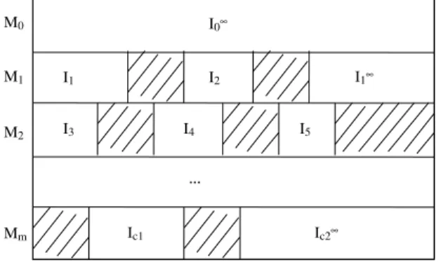
Fig. 1. An example illustrating the bounded and unbounded available intervals.
increasing the objective value too much, and thus derive our PTAS. This may give some insights for other related problems or performance criteria.
Organization.Our paper is organized as follows. In Section 2, we present our main result, which is a PTAS for P1,m
,
hk1,
hk2, . . . ,
hkm|
nr−
a, w
i=
pi|
∑
w
iCi, and then we show that there is no FPTAS for this problem. In Section3, we extend our PTAS to solve the problemP0,m,
hk1,
hk2, . . . ,
hkm|
nr−
a,
fixed, w
i=
pi|
∑
w
iCi. In Section4, we draw our conclusions.2. Preventive model
In this section, we study the case that the machine unavailability is due to preventive maintenance. We first describe our main result, a PTAS forP1,m
,
hk1,
hk2, . . . ,
hkm|
nr−
a, w
i=
pi|
∑
w
iCi. Then we show this problem does not admit an FPTAS.For each machine, its availability can be described as a sequence of alternating available intervals and unavailable intervals; all the intervals are bounded except the last, which may be available or unavailable. Letc1be the total number
of thebounded available intervalson machinesM1
,
M2, . . . ,
Mm. We use I1, . . . ,
Ic1 to denote these intervals and their lengths, and letsibe the starting time of intervalIi. It is easy to see thatc1is bounded by the total number of unavailableintervals
∑
hki. Letc2
(
c2≤
m)
be the total number of unbounded available intervals on machinesM1,
M2, . . . ,
Mm, andwe useI1∞
, . . . ,
Ic2∞to denote these intervals, respectively. Since machineM0is always available, we useI0∞to denote thisunbounded available interval. SeeFig. 1for an illustration.
LetSbe any feasible schedule of the job setJ
= {
1,
2, . . . ,
n}
, wherepi=
w
ifor alli, 1≤
i≤
n. The scheduleSassigns each job to an available interval. To minimize the total weighted completion time, it is sufficient to assume thatSdoes not contain any idle time between the jobs in each interval. Furthermore, the jobs in each available interval can be scheduled in an arbitrary order.For any set of jobsJ, letP
(
J)
be the total processing time of jobs inJ; i.e.,P(
J)
=
∑
i∈Jpi. LetQ
(
J)
be the minimum total weighted completion time of jobs inJon a single machine if jobs were continuously scheduled from time 0. Since we assume thatpi=
w
ifor alli, then the order of the jobs in the schedule does not matter, and we always haveQ
(
J)
=
−
i∈J p2i+
i̸=j−
i,j∈J pipj≥
1 2
−
i∈J pi
2=
1 2P(
J)
2.
(1)Assuming that the jobs in the same interval are always scheduled in decreasing order of their length, in this way, a schedule is uniquely determined by the assignment of all the jobs to intervals. In this paper, we will use the two terms
assignmentandscheduleinterchangeably. We will use a tuple to represent the job assignment of a schedule (maybe a partial schedule):
(
u1,
u2, . . . ,
uc1+c2+1)
, whereui, 1≤
i≤
c1, contains jobs assigned to thebounded available interval Ii, anduc1+i+1,0
≤
i≤
c2, contains jobs allocated to theunbounded available interval Ii∞. A feasible assignment (schedule) is one such that, for all available intervals, the total length of the jobs assigned to it is less than the length of the interval. Given an assignmentS
=
(
u1,
u2, . . . ,
uc1+c2+1)
, it is easy to verify that the total weighted completion time of the schedule isFw
(
S)
=
c1−
i=1(
Q(
ui)
+
siP(
ui))
+
c2−
i=0(
Q(
uc1+i+1)
+
s∞i P(
uc1+i+1))
.
(2)Treating a schedule as an assignment of the jobs gives us a new perspective of the schedules. To get a schedule of a set of jobsJ, we just need to find an assignment of the jobs to the available intervals inJ. LetJ
=
J1∪
J2. If we have an assignmentthe following facts that are used in our analysis later:
P
(
J1∪
J2)
=
P(
J1)
+
P(
J2),
(3)Q
(
J1∪
J2)
=
Q(
J1)
+
Q(
J2)
+
P(
J1)
·
P(
J2).
(4)2.1. Polynomial-time approximation scheme
Given an instance ofP1,m
,
hk1,
hk2, . . . ,
hkm|
nr−
a, w
i=
pi|
∑
w
iCiand a constant 0< ϵ <
1, our goal is to design an efficient algorithm that finds an assignment of the jobs to machines so that the total weighted completion time is at most(
1+
ϵ)
times the optimal. Our algorithm consists of four phases.1. Phase I: Assign some of the large jobs to the bounded available intervals. 2. Phase II: Assign the remaining jobs to all the available intervals.
3. Phase III: Reassign some of the jobs to make the schedule feasible.
4. Phase IV: Search for the best schedule. Both Phase I and Phase II have many alternatives, and thus result in many candidate schedules: find the one with the minimum weighted completion time.
As one can see, the main part of the algorithm lies in the first three phases, where we try to assign and reassign jobs. In Phase IV, we simply search for the best solution. In the following, we describe each of the first three phases in detail, and show how each step can be implemented efficiently.
2.1.1. Phase I: assign large jobs to bounded available intervals
First, let us define alarge job. Given a constant parameter 0
< δ <
1 which depends onϵ
, for each bounded available intervalIi(1≤
i≤
c1), we say that a job is alarge job with respect to Iiif its processing time is greater than or equal toδ
·
Ii; otherwise, it is asmall job with respect to Ii. Note that a job may be large with respect to one interval while being small with respect to another.To assign the large jobs into the bounded available intervals, we use brute force. Specifically, a job can be assigned toIi only if it is a large job with respect toIi. We enumerate all the possible assignments of large jobs to bounded intervals such that the total length of jobs assigned to the intervalIiis at mostIifor each 1
≤
i≤
c1. The following lemma gives a boundon the number of possible assignments of the large jobs.
Lemma 1. There are at most O
(
ncδ1)
possible assignments of the large jobs, where0< δ <
1is a constant depending onϵ
.Proof. For each bounded available intervalIi, the number of large jobs that can be assigned toIiis at mostIi
/(δ
Ii)
=
1/δ
. Therefore there are at mostO(
n1δ)
possible ways to assign large jobs to intervalIi. Since there arec1bounded availableintervals, there are at mostO
(
n c1δ
)
possible assignments of the large jobs to bounded available intervals in total.2.1.2. Phase II: assign remaining jobs
Once the large jobs in each bounded interval have been fixed, we assign the remaining jobs to all the available intervals, which includesc1bounded intervals andc2
+
1 unbounded intervals. For each job, we first enumerate all the possible waysto assign it, and then prune the set of assignments to reduce the number of assignments. Note that, since in Phase I we enumerate all possible ways of assigning large jobs, in this phase, a job can be assigned to a bounded interval only if it is a small job. Furthermore, in this phase, we also allow infeasible butvalidassignments; that is, the total length of jobs assigned to a bounded interval can be more than the length of the interval but at most
(
1+
δ)
times the length of the interval, whereδ
is defined as in Phase I. We say that such an interval isvalid(may be infeasible) with respect toδ
. An assignment is valid (feasible) if and only if all its intervals are valid (feasible). For each fixed large job assignment(
u1, . . . ,
uc1,
∅
,
∅
, . . . ,
∅
)
, Phase II, as described below, returns a list of valid assignments of all jobs.For each fixed large job assignment
(
u1, . . . ,
uc1,
∅
,
∅
, . . . ,
∅
)
obtained in Phase I: 1. L= {
(
u1, . . . ,
uc1,
∅
,
∅
, . . . ,
∅
)
}
.2. Repeatedly assign the remaining jobs one by one (order does not matter) until all jobs are assigned: (a) let the current remaining job bek,
(b) L′
= ∅
,(c) for each assignment
(
u1, . . . ,
uc1,
uc1+1, . . . ,
uc1+c2+1)
∈
L:for each bounded intervalIi, 1
≤
i≤
c1, such thatkis small forIi,add the assignment,
(
u1,
u2, . . . ,
ui∪ {
k}
, . . . ,
uc1+c2+1)
, toL′if it is valid,for each unbounded intervalIi∞, 0
≤
i≤
c2,add the assignment,
(
u1,
u2, . . . ,
uc1+i+1∪ {
k}
, . . . ,
uu1+c2+1)
, toL′,Letf
=
(
1+
δ2n
)
. We say that two assignments(
u1,
u2. . . ,
uc1+c2+1)
and(v
1, v
2, . . . , v
c1+c2+1)
are in the same region with respect toδ
if, for anyj, 1≤
j≤
c1+
c2+
1, there exist two integersk1,
k2, such thatfk1−1≤
P(
uj),
P(v
j) <
fk1, andfk2−1≤
Q(
uj),
Q(v
j) <
fk2.To filter the assignments, we keep from each region only one assignment as the representative. (e)L
=
L′.3. ReturnL.
Now we analyze Phase II. We have the following lemma about the relationship between any feasible schedule and the list of assignments returned by the algorithm.
Lemma 2. Let J be a set of n jobs. For any feasible schedule S
=
(
u1,
u2, . . . ,
uc1+c2+1)
of the jobs in J, after PhaseII, there existsone valid assignment
(v
1, v
2, . . . , v
c1+c2+1)
of all jobs such that the following properties hold:(1) the set of large jobs in
v
j,1≤
j≤
c1is the same as the set of large jobs in uj, denoted by ulj; (2) P(v
j)
≤
fn·
P(
uj)
,1≤
j≤
c1+
c2+
1;(3) Q
(v
j)
≤
fn·
Q(
uj)
,1≤
j≤
c1+
c2+
1.Proof. Since we enumerate all possible assignments of the large jobs, after Phase I, we must have one assignment consistent with the large job assignments inS,
(
ul1, . . . ,
ulc1,
∅
,
∅
, . . . ,
∅
)
. We will consider only the assignments of the remaining jobs that are based on this assignment. Therefore, property (1) is always true.Suppose that there aren′remaining jobs inSafter the large jobs are fixed. We prove the claim by induction onn′. When n′
=
0 the lemma is trivially true. Then we assume thatn′≥
1 and the job finishing last inSisk.Let
(
u′1
,
u′
2
, . . . ,
u′
c1+c2+1
)
be the assignment of the jobs inJ\ {
k}
by scheduleS. By inductive hypothesis, there is one validassignment of the jobs inJ
\ {
k}
, (v
′1
, v
′
2
, . . . , v
′
c1+c2+1
)
that has the following two properties.P
(v
′j)
≤
fn−1·
P(
u′j),
1≤
j≤
c1+
c2+
1;
Q
(v
j′)
≤
fn−1·
Q(
u′j),
for 1≤
j≤
c1+
c2+
1.
Suppose that, in scheduleS,kis assigned toui
,
1≤
i≤
c1+
c2+
1. This implies thatui=
u′i∪ {
k}
, and, for allj̸=
i, we haveuj=
u′j. In other words,S=
(
u1,
u2, . . . ,
uc1+c2+1)
=
(
u′1,
u′ 2
, . . . ,
u ′ i∪ {
k}
,
u ′ i+1, . . . ,
u ′ c1+c2+1)
.We consider the assignment
(v
′1
, v
′ 2, . . . , v
′ i∪ {
k}
, . . . , v
′c1+c2+1
)
. Then, by Eqs.(3)and(4)and the inductive hypothesis,we have P
(v
′i∪ {
k}
)
=
P(v
i′)
+
pk≤
fn−1P(
u′i)
+
pk=
fn−1(
P(
u′i)
+
pk)
=
fn−1P(
ui),
and Q(v
i′∪ {
k}
)
=
Q(v
i′)
+
p2k+
pk·
P(v
i′)
≤
fn−1·
Q(
u′i)
+
pk(
pk+
fn−1·
P(
u′i))
≤
fn−1(
Q(
ui′)
+
pk·
P(
ui))
=
fn−1Q(
ui).
For all intervalsIj
,
j̸=
i, the assignments are the same as before.Next, we show that this assignment is a valid assignment of all jobs with respect to
δ
. That is, we show that, for every 1≤
j≤
c1,P(v
′j)
≤
(
1+
δ)
Ij. First, for a given constantδ
, 0< δ <
1, andf=
1+
2δn, we havefn−1
<
fn=
1+
δ
2n
n< (
1+
δ),
and hence we haveP
(v
′i∪ {
k}
)
≤
fn−1P(
ui) < (
1+
δ)
Ijand, for allj̸=
i,P(v
′j)
≤
f n−1P(
u j) < (
1+
δ)
Ij, and thus(v
′ 1, v
′ 2, . . . , v
′ i∪ {
k}
, . . . , v
′c1+c2+1
)
is valid. On the other hand, if(v
′ 1
, v
′ 2, . . . , v
′ i∪ {
k}
, . . . , v
′c1+c2+1
)
is not returned by thefilter step, then another valid assignment in the same region, say
(v
1, . . . , v
c1+c2+1)
, will be returned. Since they are in thesame region, for allj, we have
P
(v
j)
≤
f·
P(v
j′)
≤
f·
f n−1P(
u j)
=
fnP(
uj)
≤
(
1+
δ)
P(
uj),
Q(v
j)
≤
f·
Q(v
j′)
≤
f·
fn −1Q(
u j)
=
fnQ(
uj).
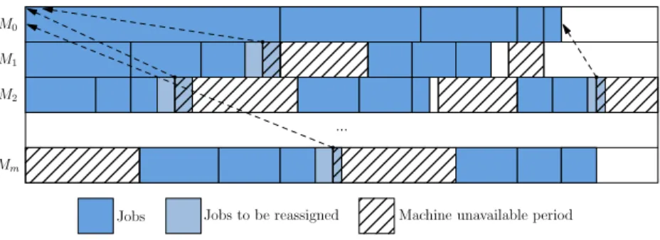
Fig. 2. An example illustrating reassignment of small jobs. The following lemma shows the time complexity of Phase II.
Lemma 3. For a fixed large job assignment, the running time of PhaseIIis O
(
n(
c1+
c2)(
logfP)
2(c1+c2+1))
, where P=
∑
pi. Proof. First, the size ofLis bounded by the total number of regions of the assignments, which isO
((
logfQ(
J)
logfP(
J))
(c1+c2+1))
. SinceQ(
J)
≤
12P
(
J)
2
=
12P
2, the number of assignments inLis at mostO
(
logfP2(c1
+c2+1)
)
. Phase II hasn′iterations to assign then′remaining jobs. If we use
(
c1
+
c2+
1)
linked lists to represent each assignment inL, the time to assign a jobto an interval is constant, and there are at mostc1
+
c2+
1 ways to assign the jobs in each assignment. Therefore the totalrunning time isO
(
n′(
c1+
c2+
1)(
logfP2(c1+c2+1)
))
=
O(
n(
c1
+
c2)(
logfP)
2(c1+c2+1)
)
.2.1.3. Phase III: reassign some jobs to make schedules feasible
Let
(
u1,
u2, . . . ,
uc1+c2+1)
be a valid assignment of all jobs after Phase II. As we mentioned before, this valid assignmentmay not be a feasible schedule because, in some bounded intervals, some jobs may be scheduled when the machine is unavailable. Hence, we want to reassign some of the jobs from these bounded available intervals to the unbounded available interval on the first machine. In Phase III, as described below, we process each valid but not feasible assignment obtained after Phase II (seeFig. 2for an illustration), and finally get a corresponding feasible assignment.
PhaseIII:reassign small jobs.
(1) Let
(
u1,
u2, . . . ,
uc1+c2+1)
be a valid but not feasible assignment of all jobs.(2) For each valid but not feasible intervalIj, i.e.,Ij
<
P(
uj) < (
1+
δ)
Ij, repeatif a job inujis scheduled at or after the timeP
(
uc1+1)
, reassign the job to machineM0, updateuc1+1anduj.(3) For each valid but infeasible intervalIjafter the above step, reassign some small jobs with total length at most 2
δ
·
Ijto machineM0; therefore it becomes feasible.We now analyze Phase III.
Lemma 4. Let S
=
(
u1,
u2, . . . ,
uc1+c2+1)
be a valid but infeasible assignment of all jobs after Phase II, and let S′=
(
u′1
,
u′
2
, . . . ,
u′
c1+1
,
uc1+2, . . . ,
uc1+c2+1)
be the feasible assignment after Phase III. Then we must have Fw(
S′)
≤
(
1+
8δc12(1−δ)2
)
Fw(
S)
.Proof. Let
(
uˆ
1,
uˆ
2, . . . ,
uˆ
c1+1,
uc1+2, . . . ,
uc1+c2+1)
be the assignment after step (2), andSˆ
be the corresponding schedule.First, note that, if a job is reassigned in step (2), its completion time will not be increased; thus we haveFw
(
Sˆ
)
≤
Fw(
S)
. LetIjbe an infeasible interval(
sj,
tj)
after step (2). We assume that all jobs are scheduled in decreasing order of their lengths. Then the last job must be a small job, whose length is at mostδ
Ij. Furthermore, it starts beforeP(
uˆ
c1+1)
, and finishes aftertj but beforetj+
δ
Ij. Hence we must haveIj<
tj<
P(
uˆ
c1+1)
+
δ
Ij; i.e., ifIjis infeasible after step (2), thenIj≤
P(uˆc1+1)
1−δ . In step (3), some small jobs are reassigned. The order of these reassigned jobs does not matter, but, for ease of analysis, we assume that these jobs are all inserted from time 0, first the jobs fromu
ˆ
0, then the jobs fromuˆ
1, and so on. Let the schedulebeS′.
Next, we analyze the increase of the total weighted completion time fromS
ˆ
toS′. We first analyze the jobs on machine M0 in Sˆ
. LetImax be the largest infeasible interval after step (2). Since the total length of the inserted jobs is at most(
2δ
I1+
2δ
I2+ · · ·
2δ
Ic1)
≤
2δ
c1Imax, for each job inuˆ
c1+1, its completion time is increased by at most 2δ
c1Imax. Usingthe fact thatImax
≤
P(uˆc1+1)
1−δ and Eq.(1), the total weighted completion time of all jobs fromu
ˆ
c1+1is increased by at most−
j∈ ˆuc1+1w
j·
(
2δ
c1Imax)
=
P(
uˆ
c1+1)(
2δ
c1Imax)
≤
2δ
c1P(
uˆ
c1+1)
2 1−
δ
≤
2δ
c1·
2Q(
uˆ
c1+1)
1−
δ
=
4δ
c1Q(
uˆ
c1+1)
1−
δ
.
For the reassigned small jobs fromu
ˆ
1, the total weighted completion time is not increased, since the completion time ofeach job is not increased. For the reassigned jobs fromu
ˆ
2, they are preceded by those reassigned small jobs fromuˆ
1, and thecompletion time of each job is increased by at most 2
δ
I1; thus the total increase of the total weighted completion time isat most 2
δ
I1·
2δ
I2≤
4δ
2Imax2 . Similarly, for the reassigned jobs fromuˆ
k, the total increase of the total weighted completion time is at most 4δ
2(
k−
1)
I2max. Summing this up for all bounded intervals, the total increase is at most
c1
−
k=1 4δ
2(
k−
1)
Imax2≤
2δ
2c12Imax2≤
2δ
2c2 1P(
uˆ
c1+1)
2(
1−
δ)
2≤
4δ
2c2 1Q(
uˆ
c1+1)
(
1−
δ)
2.
In summary, we have Fw(
S′)
−
Fw(
Sˆ
)
≤
4δ
c1·
Q(
uˆ
c1+1)
1−
δ
+
4δ
2c2 1Q(
uˆ
c1+1)
(
1−
δ)
2≤
8δ
c2 1Q(
uˆ
c1+1)
(
1−
δ)
2≤
8δ
c2 1(
1−
δ)
2Fw(
ˆ
S)
≤
8δ
c 2 1(
1−
δ)
2Fw(
S).
Thus,Fw(
S′)
≤
(
1+
8δc21 (1−δ)2)
Fw(
Sˆ
)
.Lemmas 2and4ensure that the assignment returned by Phase IV is feasible and has a cost close to that of the optimal schedule; see below.
Lemma 5. For any instance of P1,m
,
hk1,
hk2, . . . ,
hkm|
nr−
a, w
i=
pi|
∑
w
iCi, and any constantϵ
,0< ϵ <
1, let S∗be the optimal schedule. Let
δ
be a constant such that (16c2 1+1)δ
(1−δ)2
≤
ϵ
, and let S be the schedule returned after PhaseIV. Then,Fw
(
S)
≤
(
1+
ϵ)
Fw(
S∗)
. Proof. LetS∗=
(
u∗ 1,
u ∗ 2, . . . ,
u ∗c1+c2+1
)
denote the optimal schedule. ByLemma 2, there exists a valid assignmentS′
=
(
u′1,
u′2, . . . ,
uc1′ +c2+1)
after Phase II such that the three properties inLemma 2hold. ByLemma 4, after Phase III, we obtain a new feasible assignmentS′′such thatFw
(
S′′)
≤
(
1+
8c12δ (1−δ)2)
Fw(
S′
)
. Finally, in Phase IV, we get a feasible scheduleSsuch thatFw(
S)
≤
Fw(
S′′)
≤
(
1+
8c12δ (1−δ)2)
Fw(
S ′)
. By Eq.(2), Fw(
S′)
=
c1−
i=1(
Q(
u′i)
+
siP(
u′i))
+
c2−
i=0(
Q(
u′c1+i+1)
+
s∞i P(
u′c1+i+1))
.
By properties ofLemma 2, we haveQ
(
u′j)
≤
fn·
Q(
u∗j)
andP(
u′j)
≤
fn·
P(
u∗j)
forj=
1,
2, . . . ,
c1+
c2+
1. Therefore,Fw
(
S)
≤
1+
8c1 2δ
(
1−
δ)
2
c1−
i=1(
fn·
Q(
u∗i)
+
sifn·
P(
u∗i))
+
c2−
i=0(
fn·
Q(
u∗c1+i+1)
+
s∞i fn·
P(
u∗c1+i+1))
=
1+
8c1 2δ
(
1−
δ)
2
fn
c1−
i=1(
Q(
u∗i)
+
siP(
u∗i))
+
c2−
i=0(
Q(
u∗c1+i+1)
+
s∞i P(
u∗c1+i+1))
=
1+
8c1 2δ
(
1−
δ)
2
·
fnFw(
S∗)
≤
1+
8c1 2δ
(
1−
δ)
2
(
1+
δ)
Fw(
S∗)
=
1+
δ
+
8c1 2δ(
1+
δ)
(
1−
δ)
2
Fw(
S∗)
≤
1+
δ
+
16c1 2δ
(
1−
δ)
2
Fw(
S∗)
≤
1+
(
16c1 2+
1)δ
(
1−
δ)
2
Fw(
S∗)
=
(
1+
ϵ)
Fw(
S∗).
Theorem 6.There is a PTAS for P1,m
,
hk1,
hk2, . . . ,
hkm|
nr−
a, w
i=
pi|
∑
w
iCi, and its running time is O
(
nc δn
(
c+
m
)(
logfP)
2(c+m+1))
, whereϵ
is the relative error ratio,δ
is a constant such that (16(c2+1)δ1−δ)2
≤
ϵ
, f=
1+
2δn, P=
∑
pi, and
Proof. Lemma 5shows that our algorithm gives a
(
1+
ϵ)
-approximation for any constantϵ
. We only need to analyze the running time. Letc1≤
cbe the number of bounded intervals andc2≤
m+
1 be the number of unbounded intervals. ByLemma 1, there are at mostO
(
n c1δ
)
possible assignments of the large jobs. For each allocation of large jobs, byLemma 3, Phase II takesO(
n(
c1+
c2+
1)(
logfP)
2(c1+c2+1))
, and Phase III and Phase IV are dominated by Phase II. Therefore the totalcomputational time of our algorithm isO
(
ncδ1n(
c1+
c2+
1)(
logfP)
2(c1+c2+1))
=
O(
nc
δn
(
c+
m)(
logfP)
2(c+m+1))
.The above theorem leaves us an open question: Does an FPTAS exist for the problemP1,m
,
hk1,
hk2, . . . ,
hkm|
nr−
a, w
i=
pi
|
∑
w
iCi?. The question is answered below. The answer shows that the PTAS is the most efficient algorithm one can have.
2.2. No FPTAS
In this section, we show that the scheduling problem does not admit an FPTAS unlessP
=
NP. Theorem 7. The scheduling problem P1,2,
1,
1|
nr−
a, w
i=
pi|
∑
w
iCidoes not have an FPTAS unless P=
NP.Proof. Our approach to show the non-existence of an FPTAS is by reducing from the equal cardinality partition (EPC) problem. A similar technique has been used in other papers; for example, Korte and Schrader in their paper [15], showed that the two-dimensional knapsack problem does not have an FPTAS by reducing from EPC.
The EPC problem is defined as follows. Given a set of integersa1
, . . . ,
a2nsuch that∑
2ni=1ai
=
2A, determine if these integers can be divided into two setsA1andA2such that∑
i∈A1ai
=
∑
j∈A2aj
=
Aand|
A1| = |
A2| =
n. The EPC problem isNP-complete [4].
For a given instance of the EPC problem, we construct an instance of the scheduling problem as follows. There are three machines, M0,M1, andM2, whereM0 is always available, and M1 and M2 are not available during the interval
[
(
n+
1)
A,
2(
n+
1)
2A]
. There are 2n+
1 jobs, denoted by 0,
1, . . . ,
2n. For job 0,p0
=
w
0=
4(
n+
1)
A, and for 1≤
k≤
2n,pk
=
w
k=
A+
ak. Since∑
2nk=1pk
=
2(
n+
1)
A, it is easy to see that the equal sum partition instance has a YES answer iff there is a schedule in which job 0 is assigned toM0,njobs are assigned toM1, andnjobs are assigned toM2all before the unavailable intervalstarting at
(
n+
1)
A. The total weighted completion time of this schedule isp20
+
−
ionM1 p2i+
−
i,jonM1 pipj
+
−
ionM2 p2j+
−
i,jonM2 pipj
≤
p20+
2n−
i=1 p2i
+
−
i,jonM1[
(
ai+
A)(
aj+
A)
] +
−
i,jonM2[
(
ai+
A)(
aj+
A)
]
=
p20+
2n−
i=1 p2i
+
−
i,jonM1(
aiaj+
A2+
(
ai+
aj)
A)
+
−
i,jonM2(
aiaj+
A2+
(
ai+
aj)
A)
=
p20+
2n−
i=1(
A+
ai)
2
+
n(
n−
1)
A2+
(
n−
1)
−
ionM1 Aai
+
(
n−
1)
−
ionM2 Aai
+
−
i,jonM1 aiaj
+
−
i,jonM2 aiaj
≤
p20+
2n−
i=1(
A2+
2Aai+
a2i)
+
n(
n−
1)
A2+
(
n−
1)
A 2n−
i=1 ai+
1 2
−
ionM1 ai
2+
1 2
−
ionM2 ai
2≤
p20+
2nA2+
4A2+
2n−
i=1 ai
2+
n(
n−
1)
A2+
2(
n−
1)
A2+
A2=
16(
n+
1)
2A2+
2nA2+
4A2+
4A2+
(
n2+
n−
1)
A2=
(
17(
n+
1)
2+
n+
6)
A2.
On the other hand, if there is no solution to the instance of ECP, then, besides job 0, at least one other jobkhas to be scheduled onM0. Without loss of generality, we can assume thatn1jobs are scheduled onM1,n2jobs are scheduled onM2,
and thatn1
+
n2=
2n−
1. Then the total weighted completion time isp20
+
p0pk+
2n−
j=1 p2j+
−
i,jonM1 pipj+
−
i,jonM2 pipj=
p20+
p0pk+
2n−
j=1 p2j+
−
i,jonM1(
A+
ai)(
A+
aj)
+
−
i,jonM2(
A+
ai)(
A+
aj)
=
p20+
p0pk+
2n−
j=1 p2j+
−
i,jonM1(
aiaj+
A2+
(
ai+
aj)
A)
+
−
i,jonM2(
aiaj+
A2+
(
ai+
aj)
A)
=
p20+
p0pk+
2n−
j=1 p2j+
n1(
n1−
1)
A 2 2+
−
i,jonM1(
aiaj+
(
ai+
aj)
A)
+
n2(
n2−
1)
A 2 2+
−
i,jonM2(
aiaj+
(
ai+
aj)
A)
≥
p20+
p0pk+
2n−
j=1(
A+
aj)
2+
(
n21−
n1+
n22−
n2)
A2 2≥
p20+
p0pk+
2n−
j=1(
A2+
2Aaj)
+
(
n21+
(
2n−
n1−
1)
2−
(
2n−
1))
A2 2≥
p20+
p0pk+
2n−
j=1(
A2+
2Aaj)
+
(
2n−
1)(
2n−
3)
A2 4=
p20+
p0pk+
(
2nA2+
4A2)
+
(
2n−
1)(
2n−
3)
A2 4≥
(
4A(
n+
1))
2+
4(
n+
1)
AA+
(
2nA2+
4A2)
+
(
n2−
2n)
A2≥
(
16(
n+
1)
2+
n2+
4n+
8)
A2=
(
17(
n+
1)
2+
2n+
7)
A2.
Thus, if there exists an FPTAS for the scheduling problem with approximation ratio less than(17(n(+1)2+n+6)A2+(n+1)A2
17(n+1)2+n+6)A2
=
1+
(n+1)17(n+1)2+n+6, we can solve the partition problem in polynomial time. Therefore, there is no FPTAS unlessP
=
NP. Similarly, we can show that there is no FPTAS for the case of two machines, in which one of them is always available, and the other has two unavailable intervals.Theorem 8.The scheduling problem P1,1
,
2|
nr−
a, w
i=
pi|
∑
w
iCidoes not have an FPTAS unless P=
NP. 3. Fixed job modelIn this section, we study the fixed job model. We give a PTAS for the case that each job’s weight equals to its processing time form
≥
1 parallel machines. Like the preventive model, we assume that the number of unavailable intervals due to fixed jobs is also a constant, and that the weight of each job is equal to its processing time. Unlike the preventive model, we do not require a machine that is permanently available.3.1. PTAS for P0,m
,
hk1,
hk2, . . . ,
hkm|
nr−
a,
fixed, w
i=
pi|
∑
w
iCi The algorithm forP1,m,
hk1,
hk2, . . . ,
hkm|
nr−
a, w
i=
pi|
∑
w
iCican be extended to solveP0,m,
hk1,
hk2, . . . ,
hkm|
nr−
a,
fixed, w
i=
pi|
∑
w
iCi. We treat each fixed job as an unavailable interval and then apply the same algorithm. The only difference is in the reassignment of jobs in Phase III, since now there is no permanently available machine. The small jobs from an infeasible interval are still assigned on the same machine, but reassigned to other feasible intervals or to the unbounded interval; this is instead of reassigning jobs to the first machine, as in the preventive model. See below for details.PhaseIII:reassign small jobs
1. while there is an infeasible intervalIi
2. pick a small jobjfromui(assume jobjis on machineMj) 3. letIkbe the first feasible interval onMjsuch thatP
(
uk∪
j)
≤
Ik 4. reassignjtoIkor to the unbounded interval onMjifIkdoes not existWe first analyze the increase of the total weighted completion time of the reassigned jobs from a single infeasible interval
Iion machineMj. If a job is reassigned to an interval before the intervalIi, then its completion time is decreased. Hence, we can assume that all jobs are reassigned to an interval afterIi, and that they are always scheduled at the end of the new assigned interval. Suppose that the last reassigned job fromIiis rescheduled at time
τ
i. Then the completion time of all the reassigned jobs fromIiis increased by at mostτ
i, and thus the total weighted completion time is increased by at most 2δ
Ii·
τ
i. LetJMj(τ
i)
be the set of jobs scheduled beforeτ
ionMj. Next, we give an upper bound onτ
iin terms ofP(
JMj(τ
i))
. Since allthe jobs are reassigned as early as possible and the last job can not be reassigned to any interval before
τ
i, this means that the length of idle time of these intervals is less than the length of the lastly reassigned small job, which is at mostδ
Ii. There are at mostcinfeasible intervals, and hence we haveP
(
JMj(τ
i))
≥
τ
i−
cδ
Ii≥
τ
i(
1−
cδ).
Thus, the increase of the weighted completion time for jobs inIiis at most 2
δ
Iiτ
i≤
2δ
Ii·
P(
JMj(τ
i))/(
1−
cδ)
. Similarly, we canget a bound for the increase of the weighted completion time for jobs in other infeasible intervals. Let
τ
maxbe the maximumτ
i. Summing up the increase of all the intervals on machineMj, we can bound the increase of all the reassigned jobs onMj:
−
Iiis infeasible onMj 2δ
Ii.
P(
JMj(τ
i))
1−
cδ
=
2δ
1−
cδ
·
−
Iiis infeasible onMj Ii
·
P(
JMj(τ
max))
≤
2δ
1−
cδ
·
(τ
max·
P(
JMj(τ
max)))
≤
2δ
1−
cδ
·
P(
JMj(τ
max))
1−
cδ
·
P(
JMj(τ
max))
≤
2δ
(
1−
cδ)
22Q(
JMj(τ
max))
≤
4δ
(
1−
cδ)
2−
kscheduled onMjw
kCk.
Thus the total increase of all the reassigned jobs among all machines is at most( 4δ
1−cδ)2timesFw
(
S)
. For any constantϵ
, if we letδ
be a constant such that( 4δ1−cδ)2
≤
ϵ
and apply the algorithm, then we get a(
1+
ϵ)
approximation within polynomial time.Theorem 9. There is a PTAS for P0,m
,
hk1,
hk2, . . . ,
hkm|
nr−
a,
fixed, w
i=
pi|
∑
w
iCi, and its running time isO
(
ncδn(
c+
m)(
logfP)
(c+m))
, whereϵ
is the relative error ratio,δ
is a constant such that 4δ(1−cδ)2
≤
ϵ
, f=
1+
2δn, P=
∑
pi,
and c is the number of fixed jobs.
Proof. Letc1
≤
cbe the number of bounded intervals andc2=
mbe the number of unbounded intervals. ByLemma 1, thereare at mostO
(
n c1δ
)
possible assignments of the large jobs, whereδ
is a constant such that( 4δ1−cδ)2
≤
ϵ
. For each allocation of large jobs, byLemma 3, Phase II takesO(
n((
c1+
m)(
logfP)
(c1+m)))
, wheref=
1+
2δn. Therefore, the total computational time of our algorithm isO(
nc1 δn
(
c1+
c2)(
logfP)
(c1 +c2))
=
O(
ncδn(
c+
m)(
log fP)
(c +m))
. 4. ConclusionIn this paper, we have studied scheduling problems in two closely related machine availability models, the preventive model and the fixed job model. We investigate the problems of minimizing the total weighted completion time on parallel machines. For the preventive model, we assume there is one machine permanently available and that the processing time of each job is equal to its weight for all jobs. We develop the first PTAS when the number of machines and the number of unavailable intervals are both constants. Then we show that this is the best one can hope for by proving that there is no FPTAS in this case unlessP
=
NP. For the fixed job model, since there does not exist a constant approximation algorithm when the jobs’ weights are arbitrary, we concentrate on the case that the processing time of each job is equal to its weight for all jobs, and we show that the PTAS for the preventive model can be extended to solve this problem when the number of fixed jobs and the number of machines are both constants. It should be noted that, in the fixed job model, all machines can have unavailable intervals due to a priori job assignment.Our PTASs in both models work only if
w
i=
pifor all jobs. An open question for both models is to determine whether there exist approximation algorithms when the jobs have arbitrary weights assuming that one machine is permanently available.References
[1] I. Adiri, J. Bruno, E. Frostig, A.H.G. Rinnooy Kan, Single machine flow-time scheduling with a single breakdown, Acta Informatica 26 (1989) 679–696. [2] J. Blacewicz, M. Drozdowski, P. Formanowicz, W. Kubiak, G. Schmidt, Scheduling preemptable tasks on parallel processors with limited availability,
Parallel Computing 26 (9) (2000) 1195–1211.
[3] J. Breit, G. Schmidt, V.A. Strusevich, Non-preemptive two-machine open shop scheduling with non-availability constraints, Mathematical Methods of Operations Research 57 (2003) 217–234.
[4] M. Cieliebak, St. Eidenbenz, A. Pagourtzis, K. Schlude, Equal Sum Subsets: Complexity of Variations, Technical Report 370, CS, ETHZ, 2002.
[5] F. Diedrich, K. Jansen, Improved approximation algorithms for scheduling with fixed jobs, in: Proceedings of the Twentieth Annual ACM-SIAM Symposium on Discrete Algorithms, SODA, 2009, pp. 675–684.
[6] B. Fu, Y. Huo, H. Zhao, Exponential inapproximability and FPTAS for scheduling with availability constraints, Theoretical Computer Science 410 (2009) 2663–2674.
[7] B. Fu, Y. Huo, H. Zhao, Makespan minimization with machine availability constraints, Discrete Mathematics, Algorithms and Applications 1 (2) (2009) 141–151.
[8] I. Kacem, Approximation algorithm for the weighted flow-time minimization on a single machine with a fixed non-availability interval, Computers & Industrial Engineering 54 (2008) 401–410.
[9] I. Kacem, C. Chu, Worst-case analysis of the WSPT and MWSPT rules for single machine scheduling with one planned setup period, European Journal of Operational Research 187 (3) (2008) 1080–1089.
[10] I. Kacem, H. Kellerer, Fast approximation algorithms to minimize a special weighted flow-time criterion on a single machine with a non-availability interval and release dates, Journal of Scheduling (2009)doi:10.1007/s10951-009-0146-4.
[11] I. Kacem, R. Mahjoub, Fully polynomial time approximation scheme for the weighted flow-time minimization on a single machine with a fixed non-availability interval, Computers & Industrial Engineering 56 (4) (2008) 1708–1712.
[12] M. Kaspi, B. Montreuil, On the Scheduling of Identical Parallel Processes with Arbitrary Initial Processor Available Times, Reserach Report 88-12, School of Industrial Engineering, Purdue University, 1988, 1988.
[13] H. Kellerer, Algorithm for multiprocessor scheduling with machine release time, IIE Transactions 30 (1998) 991–999.
[14] H. Kellerer, V.A. Strusevich, Fully polynomial approximation schemes for a symmetric quadratic knapsack problem and its scheduling applications, Algorithmica 57 (4) (2010) 769–795.
[15] B. Korte, R. Schrader, On the existence of fast approximation schemes, in: Proceedings of the 4th Symposium, Madison, Wisc, Nonlinear Programming, vol. 4, Academic Press, 1980, pp. 415–437.
[16] C.Y. Lee, Machine scheduling with availability constraint, Journal of Global Optimization 9 (1996) 395–416.
[17] C.Y. Lee, Machine scheduling with availability constraints, in: J.Y.-T Leung (Ed.), Handbook of Scheduling, CRC Press, 2004, pp. 22.1–22.13. [18] C.Y. Lee, S.D. Liman, Single machine flow-time scheduling with scheduled maintenance, Acta Informatica 29 (1992) 375–382.
[19] Lu-Wen Liao, Gwo-Ji Sheen, Parallel machine scheduling with machine availability and eligibility constraints, European Journal of Operational Research 184 (2) (2008) 458–467.
[20] S. Liman, Scheduling with Capacities and Due-Dates, Ph.D. Dissertation, Industrial and Systems Engineering Department, University of Florida, 1991. [21] C. Sadfi, M.-D. Aroua, B. Penz, Single machine total completion time scheduling problem with availability constraints, in: Proceedings of the Ninth
International Workshop on Project Management and Scheduling, PMS’2004, Nancy, France, 2004, pp. 147–150.
[22] H. Saidy, M. Taghvi-Fard, Study of scheduling problems with machine availability constraint, Journal of Industrial and Systems Engineering 1 (4) (2008) 360–383.
[23] M. Scharbrodt, A. Steger, H. Weisser, Approximation of scheduling with fixed jobs, Journal of Scheduling 2 (1999) 267–284. [24] G. Schmidt, Scheduling with limited machine availability, European Journal of Operational Research 121 (2000) 1–15.
[25] J. Yuan, Y. Lin, C. Ng, T. Cheng, Approximability of single machine scheduling with fixed jobs to minimize total completion time, European Journal of Operational Research 178 (1) (2007) 46–56.