Scheduling with communication for
multiprocessor computation
Scheduling met communicatie voor multiprocessor berekeningen
(met een samenvatting in het Nederlands)Proefschrift
ter verkrijging van de graad van doctor aan de Universiteit Utrecht
op gezag van de Rector Magnificus, Prof. dr. H.O. Voorma, ingevolge het besluit van het College voor Promoties
in het openbaar te verdedigen
op woensdag 10 juni 1998 des ochtends te 10.30 uur
door
Jacobus Hendrikus Verriet
geboren op 3 oktober 1970 te Ubbergen
Promotor: Prof. dr. J. van Leeuwen
Faculteit Wiskunde & Informatica Co-promotor: Dr. M. Veldhorst
Faculteit Wiskunde & Informatica
Contents
Contents iii
Introduction
1
1 Introduction 3
1.1 Communication in parallel computers . . . 4
1.2 Multiprocessor scheduling . . . 4
1.3 Models of parallel computation . . . 5
1.3.1 Shared memory models . . . 6
1.3.2 Distributed memory models . . . 7
1.4 An overview of the thesis . . . 8
2 Preliminaries 9 2.1 Precedence graphs . . . 9
2.2 General scheduling instances . . . 10
2.3 Communication-free schedules . . . 11
2.4 Approximation algorithms . . . 12
2.5 Special precedence graphs . . . 13
2.5.1 Tree-like task systems . . . 13
2.5.2 Interval orders . . . 14
I
Scheduling in the UCT model
15
3 The Unit Communication Times model 17 3.1 Communication requirements . . . 17 3.2 Non-uniform deadlines . . . 17 3.3 Problem instances . . . 18 3.4 Feasible schedules . . . 18 3.5 Tardiness . . . 22 3.6 Previous results . . . 233.7 Outline of the first part . . . 24
4 Individual deadlines 25 4.1 Consistent deadlines . . . 25
4.2 Computing consistent deadlines . . . 30
4.2.1 A restricted number of processors . . . 30
4.2.2 An unrestricted number of processors . . . 33
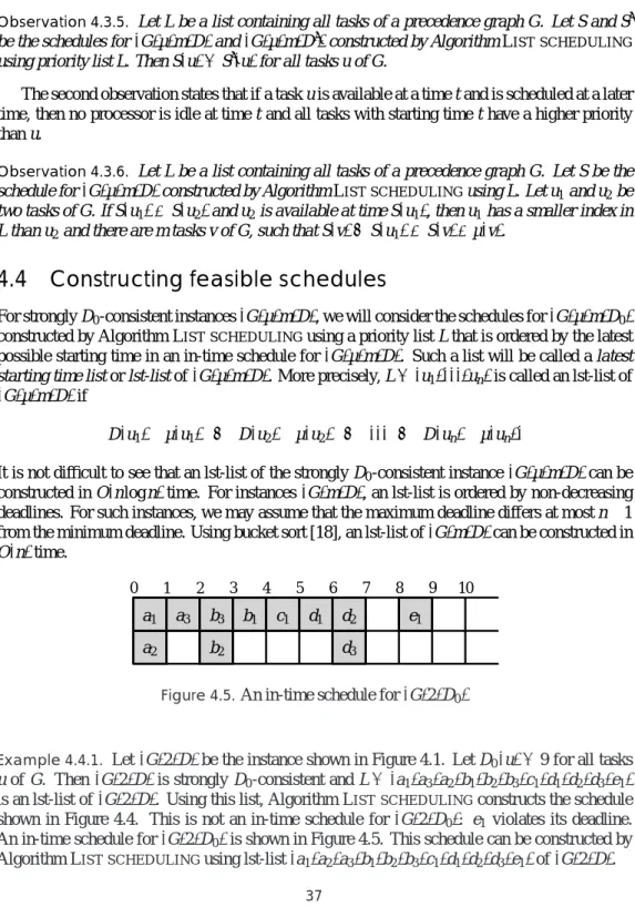
4.4 Constructing feasible schedules . . . 37
4.4.1 Arbitrary graphs on a restricted number of processors . . . 38
4.4.2 Arbitrary graphs on an unrestricted number of processors . . . 42
4.4.3 Outforests on a restricted number of processors . . . 43
4.4.4 Outforests on an unrestricted number of processors . . . 47
4.5 Concluding remarks . . . 48
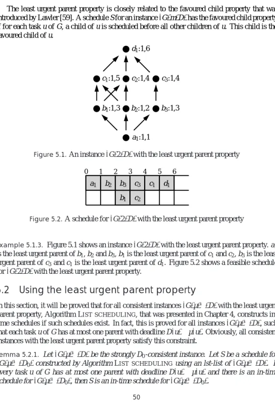
5 The least urgent parent property 49 5.1 The least urgent parent property . . . 49
5.2 Using the least urgent parent property . . . 50
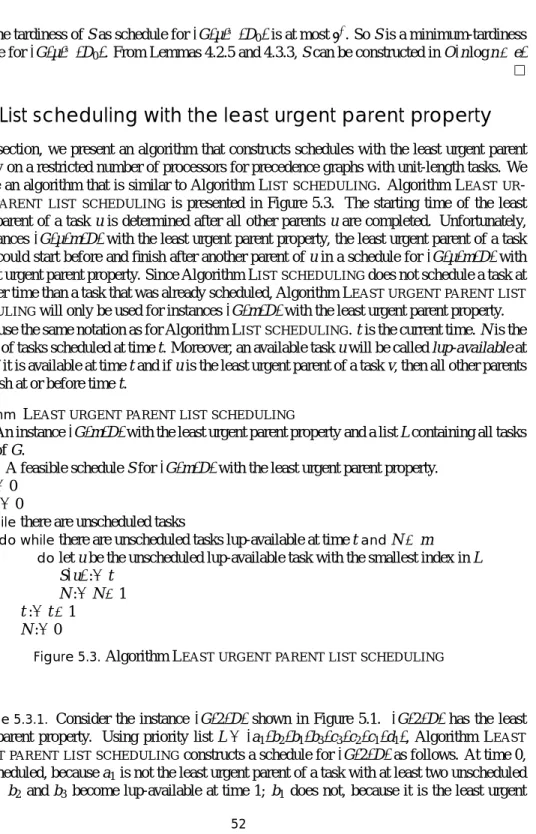
5.3 List scheduling with the least urgent parent property . . . 52
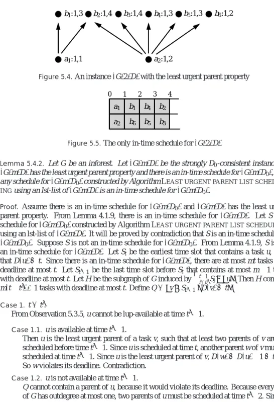
5.4 Inforests . . . 55
5.4.1 Constructing minimum-tardiness schedules . . . 55
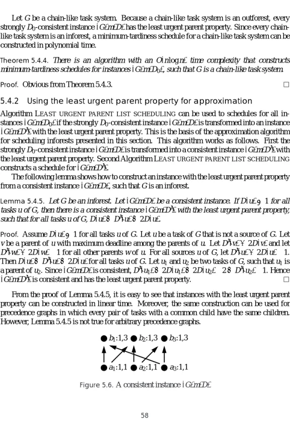
5.4.2 Using the least urgent parent property for approximation . . . 58
5.5 Concluding remarks . . . 60
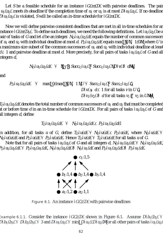
6 Pairwise deadlines 61 6.1 Pairwise consistent deadlines . . . 61
6.2 Computing pairwise consistent deadlines . . . 67
6.2.1 Arbitrary precedence graphs . . . 67
6.2.2 Interval-ordered tasks . . . 71
6.3 Constructing minimum-tardiness schedules . . . 76
6.3.1 Precedence graphs of width two . . . 76
6.3.2 Interval-ordered tasks . . . 79
6.4 Concluding remarks . . . 82
7 Dynamic programming 83 7.1 Decompositions into chains . . . 83
7.2 A dynamic-programming algorithm . . . 86
7.3 An NP-completeness result . . . 91
7.4 Another dynamic programming algorithm . . . 93
7.5 Concluding remarks . . . 99
II
Scheduling in the LogP model
101
8 The LogP model 103 8.1 Communication requirements . . . 1038.2 Problem instances . . . 104
8.3 Feasible schedules . . . 105
8.4 Previous results . . . 109
9 Send graphs 111
9.1 An NP-completeness result . . . 111
9.2 A 2-approximation algorithm . . . 113
9.3 A polynomial special case . . . 117
9.4 Concluding remarks . . . 120
10 Receive graphs 123 10.1 An NP-completeness result . . . 123
10.2 Two approximation algorithms . . . 124
10.2.1 An unrestricted number of processors . . . 124
10.2.2 A restricted number of processors . . . 130
10.3 A polynomial special case . . . 134
10.4 Concluding remarks . . . 136
11 Decomposition algorithms 137 11.1 Decompositions of intrees . . . 137
11.2 Scheduling decomposition forests . . . 140
11.3 Constructing decompositions of intrees . . . 145
11.3.1 β-restricted instances . . . 145
11.3.2 Constructing decompositions of d-ary intrees . . . 147
11.3.3 Constructing decompositions of arbitrary intrees . . . 151
11.4 Concluding remarks . . . 155
Conclusion
157
12 Conclusion 159 12.1 Scheduling in the UCT model . . . 15912.2 Scheduling in the LogP model . . . 160
12.3 A comparison of the UCT model and the LogP model . . . 161
Bibliography 163
Acknowledgements 169
Samenvatting 171
Curriculum vitae 173
1
Introduction
Scheduling is concerned with the management of resources that have to be allocated to activi-ties over time subject to a number of constraints. A (feasible) schedule is an allocation of the resources to the activities that satisfies all constraints. The objective of scheduling is finding a schedule that is optimal with respect to a certain objective function. The resources that have to be allocated and the constraints that have to be satisfied can be of various types. Hence many real-life problems can be viewed as scheduling problems.
Crew scheduling. An airline company must allocate personnel (pilots and flight attendants) to flights, such that the number of pilots and flight attendants is sufficient on each flight, each employee has a (flight-dependent) period of time off between two flights and each employee returns home regularly. An objective of crew scheduling could be minimising the number of employees and equally dividing the working hours among the personnel.
Classroom scheduling. A school has to allocate teachers and classrooms to courses, such that no teacher is in two classrooms at the same time, no course gets assigned two teachers or two classrooms, no teacher works more than seven hours on one day and no student has more than seven courses on one day. The objective of classroom scheduling could be minimising the total amount of time that the teachers and the students have to be at school.
Vehicle routing. A transport company must allocate trucks to goods that have to be transported, such that the volume of the goods on one truck does not exceed its capacity, all trucks return at their depot at the end of each day, no truck driver works more than eight hours on one day and all goods are loaded and unloaded during office hours. The objective of vehicle routing could be minimising the number of trucks.
In general, a scheduling problem assumes the existence of a set of operations (the activities) and a set of machines (the resources). The machines have to be assigned to the operations over time subject to a number of constraints.
Machine scheduling. A machine must be allocated to each operation, such that no machine is assigned to two operations at the same time and exactly one machine is assigned to each operation.
All scheduling problems are generalisations of the machine scheduling problem. For example, in crew scheduling, the personnel corresponds to the machines and the flights to the operations.
This thesis is concerned with multiprocessor scheduling, the problem of executing a computer program on a parallel computer.
Multiprocessor scheduling. The processors of a parallel computer have to be allocated to the tasks of a computer program, such that no processor executes two tasks at the same time and every task is executed exactly once.
Usually, a multiprocessor schedule has to satisfy some additional constraints.
Multiprocessor scheduling is a generalisation of machine scheduling: the processors corre-spond to the machines and the tasks to the operations.
1.1
Communication in parallel computers
This thesis is concerned with multiprocessor scheduling with communication. This is an essen-tial aspect of the problem of executing a computer program on a parallel computer. A computer program can be seen as a collection of instructions. These include assignments, arithmetic in-structions, conditional statements, loop statements and subroutine calls. We will assume that the instructions are combined into clusters. These clusters of instructions will be called tasks.
A parallel computer can be viewed as a collection of processors and memories and a com-munication mechanism; in this thesis, we will not consider the other components of a parallel computer. The processors are used to execute the tasks of a computer program. The memo-ries are used to store data. The communication mechanism is used to transfer data between the components (processors and memories) of the parallel computer.
There are two types of parallel computer that differ in the way memory is used. In a dis-tributed memory computer, each processor has a local memory. The processors of a disdis-tributed memory computer are connected by a communication network, but are not a part of this network. In shared memory computers, there is a global memory that is used by all processors.
The communication mechanisms of these computers are different. In both models, a data transfer can be viewed as a sequence of communication operations. In a shared memory com-puter, data is transferred from a source processor to a destination processor by writing and read-ing in shared memory. A data transfer consists of a write operation followed by a read operation. The source processor writes the data in a memory location, after which it can be read by the des-tination processor. The write operation does not interfere with the availability of the desdes-tination processor. Similarly, the source processor is not involved in the execution of the read operation. Because simultaneous access of a memory location by two processors is not allowed, the dura-tion of the write and read operadura-tions depends on the number of processors that want to access the same memory location simultaneously.
In a distributed memory computer, data is transferred by sending messages from one proces-sor to another through the communication network. In such computers, a data transfer consists of three communication operations: a send operation, a transport operation and a receive op-eration. The send operation is executed by the source processor; the send operation submits a message to the communication network. The transport operation is used to transport a message over the connections in the communication network from the source processor to the destination processor. No processor is involved in the execution of the transport operation. After a mes-sage has been transported, the destination processor can obtain the data from the mesmes-sage by executing a receive operation. The duration of the send and receive operations depends on the size of a message. The duration of a transport operation varies with the size of the message, the distance between the source and the destination processor, the capacity of the connections in the communication network and the number of messages that reside in the communication network.
1.2
Multiprocessor scheduling
During the execution of a computer program on a given input, each task has to be executed by one processor and the duration of its execution depends on the input. Some of the tasks have
to be executed in a specified order, because the result of a task may be needed to execute other tasks. Such tasks will be called data dependent. Other tasks can be executed in an arbitrary order or simultaneously on different processors of a parallel computer. If two data-dependent tasks are executed on different processors, then the result of the first task must be transported to the processor that executes the other task using the communication mechanism.
Multiprocessor scheduling can be viewed as a generalisation of the machine scheduling prob-lem. The machines are the processors and the components of the communication mechanism of the parallel computer. The operations are the tasks and the communication operations. Proces-sors and components of the communication mechanism have to be allocated to each task and each communication operation for some period of time. Each task and every send and receive operation has to be assigned a processor on which it is executed. The write and read operations have to be allocated a processor and a memory location that must be accessed. A sequence of connections in the communication network has to be assigned to every transport operation: these connections form the path over which the corresponding message is sent through the communi-cation network.
An assignment of processors and components of the communication mechanism to the tasks and the communication operations has to satisfy many constraints. Usually,
1. no processor can execute two tasks or communication operations at the same time; 2. data-dependent tasks cannot be executed at the same time;
3. if two data-dependent tasks are executed on different processors, then a data transfer must be executed between these tasks;
4. if communication is modelled by writing and reading messages in shared memory, then (a) no shared memory location can be accessed by two processors at the same time; and (b) a task cannot be executed until all data for this task is read by the processor on which
it is executed; and
5. if communication between the processors is modelled by sending messages through a com-munication network, then
(a) the number of messages sent over a connection of the network at the same time may not exceed the capacity of the connection; and
(b) a task cannot be executed until all messages required for this task are received by the processor on which it is executed.
Apart from the large number of constraints that need to be satisfied, there are also many objective functions that could be minimised or maximised. The most common of these is the minimisation of the makespan, the duration of the execution of the computer program.
1.3
Models of parallel computation
Because of the large number of different constraints in multiprocessors scheduling and the great variety of parallel computer architectures, it is difficult to design efficient algorithms that
con-struct good multiprocessor schedules. This is the reason to introduce an abstract model of a parallel computer, a model of parallel computation. In such a model, one can concentrate on those aspects in multiprocessor scheduling that have a large impact on the objective function (for instance, the makespan). A good model of parallel computation helps to understand the essence of the problem of multiprocessor scheduling with communication.
If the duration of the tasks is large compared to the duration of the communication operations, then the impact of communication on most objective functions is small. For such problems, we can use a model of parallel computation in which all communication constraints are removed. In this model, the duration of the communication operations is assumed to be negligible. A schedule for a computer program in this model is an allocation of processors over time, such that no processor executes two tasks at the same time and data-dependent tasks are executed in the right order. This is the most common scheduling model. Lawler et al. [60] give an overview of the work on scheduling without communication requirements subject to many additional constraints and several objective functions.
In a real parallel computer, sending a message through the communication network or access-ing a shared memory location is a very costly operation compared to a simple arithmetic opera-tion. So the communication-free model of parallel computation does not capture the complexity of parallel computation. Many other models have been presented that incorporate communica-tion in some way. An overview of such models is presented in the remainder of this seccommunica-tion. The communication constraints of the models based on shared memory parallel computers are described in Section 1.3.1 and those of the models based on distributed memory computers in Section 1.3.2. Guinand [40] and Juurlink [51] have presented more elaborate overviews of mod-els of parallel computation.
1.3.1
Shared memory models
Most shared memory models are generalisations of the Parallel Random Access Machine intro-duced by Fortune and Wyllie [28]. The PRAM is the most common model of parallel compu-tation. A PRAM consists of an infinite collection of identical processors that each have an un-limited amount of local memory. The processors execute a computer program in a synchronous manner: all processors start a task or a communication operation at the same time. The proces-sors communicate by writing and reading in shared memory. Two procesproces-sors can read the same memory location simultaneously, but a memory location cannot be written by one processor and written or read by another processor at the same time. This model of parallel computation is also called the Concurrent Read Exclusive Write PRAM. Snir [82] introduced two variants of the PRAM model: the Exclusive Read Exclusive Write PRAM in which no simultaneous access of the same memory location is allowed, and the Concurrent Read Concurrent Write PRAM in which a memory location can be read or written by several processors at the same time.
The PRAM model does not capture the complexity of communication in the execution of computer programs: a communication operation has the same duration as the execution of a com-putation instruction whereas in a real parallel computer, a communication operation is far more time consuming. There are several PRAM-based models of parallel computation that include other aspects of real parallel computers. Asynchronous variants of the PRAM were presented by Cole and Zajicek [15, 16] and by Gibbons [34]. In an asynchronous PRAM, the processors need
not start the execution of an instruction or a communication operation simultaneously. Hence processors executing a simple arithmetic instruction do not have to wait for processors that are reading or writing in shared memory.
Most PRAM-based models of parallel computation include a more realistic representation of shared memory access than the PRAM itself. The Delay PRAM introduced by Martel and Raghu-natham [65] and the Local-Memory PRAM of Aggarwal et al. [3] extend the PRAM model by including a latency for shared memory access. In these models, the duration of a communication operation is fixed and larger than the duration of an arithmetic operation. The Queue Read Queue Write PRAM presented by Gibbons et al. [35, 36] includes memory contention: it is allowed to access the same shared memory location simultaneously, but the duration of a memory access depends on the number of processors that want to read or write the same memory location. In the Block Parallel PRAM of Aggarwal et al. [2], accessing a consecutive block of shared memory locations is less time consuming than separately accessing these memory locations: the duration of a write or read operation equals the sum of a fixed latency and a function linear in the number of consecutive memory locations that must be accessed.
1.3.2
Distributed memory models
In the execution of a computer program on a distributed memory computer, each task is executed by one processor and messages are sent through the communication network. For each pair of data-dependent tasks scheduled on different processors, one needs to assign a path through the communication network that will be used to send messages. This is known as routing. In this thesis, the problem of routing will be ignored.
The simplest model of parallel computation based on a distributed memory parallel computer is a model in which the communication network is a complete graph (there is a direct connection between every pair of processors) and each connection in the communication network has an unbounded capacity. In this model, transporting a message from one processor to another takes a fixed amount of time. The communication is represented by the duration of the transport operations only; the duration of the send and receive operations is assumed to be zero. For multiprocessor scheduling, this is the most common model of parallel computation that does not neglect the communication costs. It was introduced by Rayward-Smith [79]. An overview of scheduling problems in this model is given by Chr´etienne and Picouleau [13].
This basic model has been generalised in several ways. Papadimitriou and Yannakakis [75] assume that the fixed duration of the transport operations depends on the topology of the commu-nication network. Finta and Liu [25, 26] and Picouleau [78] add an overall capacity constraint: the number of messages that can be sent through the communication network at the same time is bounded. Kalpakis and Yesha [52, 53], Cosnard and Ferreira [19] and Bampis et al. [6] con-sider models of parallel computation in which the communication network is not a complete graph: the duration of transport operations in such networks depends on the distance between the communicating processors.
Most models of parallel computation include only one or two aspects of real parallel com-puters, but some include more aspects. These models are all architecture independent and char-acterise the execution of computer programs on a real parallel computer by a small number of parameters. The Bulk Synchronous Parallel model was introduced by Valiant [85]. The BSP
model is a synchronous model of parallel computation in which the synchronisation costs are not neglected. These costs are modelled by a communication latency. In addition, the number of messages that can be sent at the same time is bounded by the throughput of the communication network, and the duration of send or receive operations is not negligible.
The Postal model was introduced by Bar-Noy and Kipnis [7]. It includes communication overheads and communication latencies: the send and receive operations have unit length and the transport operations have a fixed duration that depends on the network topology.
The LogP model was introduced by Culler et al. [21]. The LogP model is named after its parameters: the latency L, the overhead o, the gap g and the number of processors P. The LogP model is more general than the Postal model. Like in the Postal model, the transport operations in the LogP model have a fixed duration that depends on the topology of the communication net-work. Sending and receiving a message of unit size takes a fixed amount of time. The bandwidth of a parallel computer is modelled as well: there is a minimum delay between two consecutive send and receive operations executed on the same processor.
1.4
An overview of the thesis
This thesis consists of four parts: an introductory part, two main parts and a concluding part. The introductory part consists of Chapters 1 and 2. In these chapters, the terminology and notation used in the main parts are presented. The two main parts (Parts I and II) are concerned with scheduling in two different models of parallel computation and subject to two different objective functions. These parts are self-contained and can therefore be read separately. The concluding part consists of Chapter 12.
Part I consists of Chapters 3, 4, 5, 6 and 7. In these chapters, we study the problem of constructing minimum-tardiness schedules in the Unit Communication Times model, the model of parallel computation in which communication is represented by a latency of unit length. The computer programs that are to be scheduled in this model consist of tasks that have been assigned a deadline. The UCT model is introduced in Chapter 3. In the remaining chapters of Part I, we present several algorithms that construct minimum-tardiness schedules (schedules in which the maximum amount of time by which a deadline is exceeded is as small as possible) for special classes of data dependencies.
Part II is concerned with the problem of constructing minimum-length schedules in the LogP model. This part consists of Chapters 8, 9, 10, and 11. Chapter 8 is used to introduce the LogP model. In the remaining chapters of Part II, the complexity of constructing minimum-length schedules in the LogP model is studied. It is proved that this problem is NP-hard even for a restricted class of data dependencies. Moreover, in Part II, we present the first approximation algorithms with a constant approximation ratio for scheduling two special classes of data depen-dencies in the LogP model.
2
Preliminaries
In this chapter, the general notation in multiprocessor scheduling and some preliminary results are presented. In Section 2.1, we present the terminology for precedence graphs that will be used throughout this thesis. Section 2.2 presents the general scheduling instances. The general notion of a schedule is given in Section 2.3. In Section 2.4, the notion of approximation algorithms for scheduling is presented. Special classes of precedence graphs and the properties of these classes of precedence graphs are presented in Section 2.5.
2.1
Precedence graphs
In the execution of a computer program on a parallel machine, each task of the program is executed by exactly one of the processors. The tasks can often not be executed in an arbitrary order: the result of a task may be needed by other tasks. If the result of task u1is needed to
execute task u2, then the execution of u1must be completed before the execution of u2can start.
If the execution of u2does not require the result of u1, then u1and u2can be executed in arbitrary
order or at the same time on different processors.
The tasks of a computer program and their data dependencies will be represented by a prece-dence graph.
Definition 2.1.1. A directed graph is a tuple G= (V,E), where V is a set of nodes and E⊆V×V is a set of arcs between the nodes. An arc is a pair of two nodes of V : the pair(u1,u2)denotes the
arc from u1to u2. A directed graph G= (V,E)is called a precedence graph or directed acyclic
graph if there is no sequence of arcs(u1,u2),(u2,u3), . . . ,(uk,u1)in E for any k≥1.
Let G= (V,E)be a precedence graph. A node from V corresponds to a task from the com-puter program. An arc from one node to another represents a data dependency between the corresponding tasks: if there is an arc from node u1to node u2, then the result of the task
corre-sponding to u1is needed to execute the task that corresponds to u2. Since there is a one-to-one
correspondence between the tasks of a computer program and the nodes in a precedence graph, we will use the term task for the nodes in a precedence graph.
Let G be a precedence graph. The set V(G)denotes the set of tasks of G and E(G)the set of arcs of G. Throughout this thesis, we will assume that V(G)contains n tasks and E(G)contains e arcs. A path in G is a sequence of k≥2 tasks u1,u2, . . . ,ukof G, such that G contains an arc from uito ui+1for all i∈ {1, . . . ,k−1}. From the definition of precedence graphs, there are no
paths in G from a task to itself. The length of a path is the number of tasks on the path. The height of G is the length of a longest path in G.
Let u1and u2be two tasks of G. u1is called a predecessor of u2 if there is a path in G
from u1to u2. In that case, u2is called a successor of u1, which is denoted by u1≺Gu2. The
sets of predecessors and successors of a task u of G are denoted by PredG(u)and SuccG(u), respectively. Tasks without successors will be called sinks and tasks without predecessors will be called sources. u2is called a child of u1if(u1,u2)is an arc of G. If u2is a child of u1, then
u1is called a parent of u2. This is denoted by u1≺G,0u2. The sets PredG,0(u)and SuccG,0(u)
contain the parents and children of u, respectively. The number of children of a task u is the outdegree of u; its indegree equals the number of parents of u. It is not difficult to prove that ∑u∈V(G)|PredG,0(u)|=∑u∈V(G)|SuccG,0(u)|=|E(G)|.
Two tasks u1and u2of G are called incomparable if neither u1≺Gu2, nor u2≺Gu1.
Other-wise, they are called comparable. The width of G is the maximum number of pairwise incom-parable tasks of G. Consequently, if G is a precedence graph of width w, then every subset of V(G)with at least w+1 elements contains at least two comparable tasks. A chain in G is a set of pairwise comparable tasks of G. Note that the tasks on a path in G form a chain and that the size of a maximum-size chain in G equals its height. A set of pairwise incomparable tasks is called an anti-chain in G. So the width of G equals the size of a maximum-size anti-chain in G. A topological order of a precedence graph G is a list containing all tasks of G, such that each task has a smaller index in the list than its successors. There is a topological order of all precedence graphs. A topological order of G can be constructed in O(n+e)time [18].
The transitive closure of G is a precedence graph G+, such that V(G+) =V(G) and E(G+) ={(u
1,u2)|u1≺Gu2}. Hence the transitive closure of G contains an arc from every
task of G to each of its successors. The transitive reduction of G is a precedence graph G−, such that V(G−) =V(G)and for all tasks u1, u2and u3of G, u1≺Gu2if and only if u1≺G−u2
and if u1≺Gu2 and u2≺Gu3, then (u1,u3)is not an arc of G−. Throughout this thesis, e−
equals the number of arcs of the transitive reduction of G and e+ the number of arcs in the transitive closure of G. A transitive closure or a transitive reduction of G can be constructed in O(min{n2.376,n+e+ne−})time [17, 37]. Transitive closures and transitive reductions of prece-dence graphs will be used to obtain more efficient implementations of algorithms.
Let U be a set of tasks of a precedence graph G. The subgraph of G induced by U is the precedence graph(U,E(G)∩(U×U)). This precedence graph is denoted by G[U]. A precedence graph H is called a subgraph of G, if there is a subset U of V(G), such that G[U]equals H. A prefix of a precedence graph G is a subset U of V(G), such that for all tasks u1and u2of G, if
u2∈U and u1≺Gu2, then u1∈U .
2.2
General scheduling instances
During the execution of a computer program, the duration of the execution of a task depends on the input of the computer program. A function µ is used to specify the execution length of every task of the computer program for a given input: for each task u of G, µ(u)is the duration of the execution of u. Hence a computer program (for a given input) will be represented by a tuple(G,µ), where G is a precedence graph and µ : V(G)→ZZ+is a function that assigns an execution length or task length to every task of G. We will assume that µ is also used to denote the total execution time of a precedence graph or a set of tasks. So if U is a set of tasks of G, then µ(U) =∑u∈Uµ(u). In addition, µ(G) =µ(V(G)) =∑u∈V(G)µ(u).
A general scheduling instance is represented by a tuple(G,µ,m), such that(G,µ)corresponds to a computer program and m∈ {2,3, . . . ,∞}equals the number of processors that is available
for the execution of this computer program. If m=∞, then the number of available processors is unrestricted. Since we assume that every task is executed by exactly one processor, instances
(G,µ,∞)correspond to instances(G,m,n). We will not consider instances(G,µ,1), because the scheduling problems that will be studied in this thesis are easily solvable on one processor.
2.3
Communication-free schedules
A schedule for a computer program corresponds to the execution of the computer program on a parallel machine for a given input. A schedule assigns a starting time and a processor to all tasks.
Definition 2.3.1. A schedule for a scheduling instance(G,µ,m)is a pair of functions(σ,π), such thatσ: V(G)→INandπ: V(G)→ {1, . . . ,m}.
Consider a schedule(σ,π)for an instance(G,µ,m).σis an assignment of starting times and πan assignment of processors.σ(u)represents the starting time of u andπ(u)the processor on which u is executed. A task u is said to be scheduled at timeσ(u)on processorπ(u). Each task has exactly one starting time. So duplication of tasks is not allowed. u starts at timeσ(u)and is completed at timeσ(u) +µ(u), its completion time. Preemption is not allowed: the execution of u cannot be interrupted and resumed at a later time. u is said to be executed at time t on processor π(u)for all times t, such thatσ(u)≤t≤σ(u) +µ(u)−1. A processor is called idle at time t if no task is executed at time t on that processor.
A feasible schedule is a schedule in which no processor executes two tasks at the same time and the comparable tasks are executed in the right order.
Definition 2.3.2. A schedule(σ,π)for(G,µ,m)is called a feasible communication-free schedule or feasible schedule for(G,µ,m)if for all tasks u16=u2of G,
1. ifπ(u1) =π(u2), thenσ(u1) +µ(u1)≤σ(u2)orσ(u2) +µ(u2)≤σ(u1); and
2. if u1≺Gu2, thenσ(u1) +µ(u1)≤σ(u2).
The first constraint states that no processor can execute two tasks at the same time. The second ensures that a task is scheduled after its predecessors.
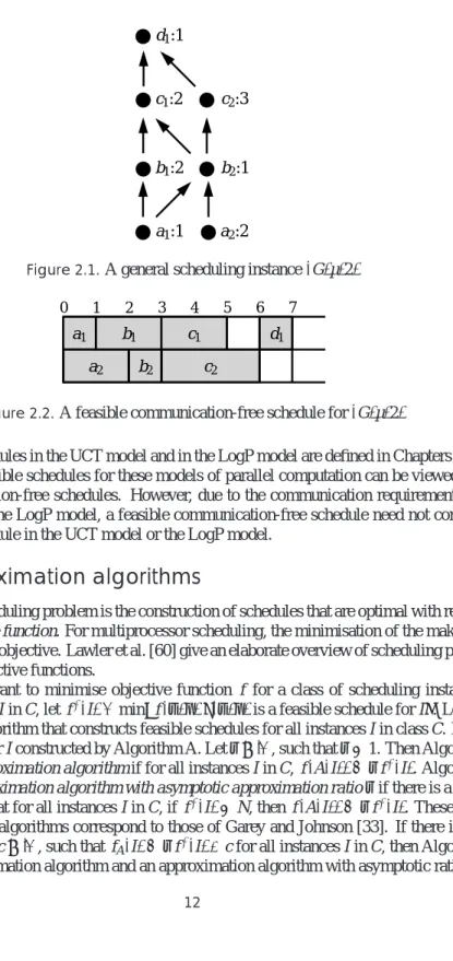
Example 2.3.3. Consider the instance(G,µ,2)shown in Figure 2.1. Every task of G is labelled with its name and its execution length. A schedule(σ,π)for(G,µ,2)is shown in Figure 2.2: σ(a1) =0,σ(a2) =0,σ(b1) =1,σ(b2) =2,σ(c1) =3,σ(c2) =3 andσ(d1) =6. Moreover,
π(a1) =π(b1) =π(c1) =π(d1) =1 andπ(a2) =π(b2) =π(c2) =2. It is not difficult to see that
this is a feasible communication-free schedule for(G,µ,2).
Let(σ,π)be a feasible (communication-free) schedule for(G,µ,m). The length or makespan of (σ,π) is the maximum completion time of a task of G; the makespan of (σ,π) equals maxu∈V(G)(σ(u) +µ(u)). (σ,π)is called a minimum-length schedule for (G,µ,m)if there is no feasible schedule for(G,µ,m)with a smaller length than(σ,π).
b1:2
c1:2 c2:3
d1:1
a1:1 a2:2
b2:1
Figure 2.1.A general scheduling instance(G,µ,2)
b2 d1 b1 c1 0 1 2 3 4 5 6 7 a1 a2 c2
Figure 2.2.A feasible communication-free schedule for(G,µ,2)
Feasible schedules in the UCT model and in the LogP model are defined in Chapters 3 and 8, respectively. Feasible schedules for these models of parallel computation can be viewed as fea-sible communication-free schedules. However, due to the communication requirements of the UCT model and the LogP model, a feasible communication-free schedule need not correspond to a feasible schedule in the UCT model or the LogP model.
2.4
Approximation algorithms
The goal of a scheduling problem is the construction of schedules that are optimal with respect to a certain objective function. For multiprocessor scheduling, the minimisation of the makespan is the most common objective. Lawler et al. [60] give an elaborate overview of scheduling problems and different objective functions.
Assume we want to minimise objective function f for a class of scheduling instances C. For each instance I in C, let f∗(I) =min{f(σ,π)|(σ,π)is a feasible schedule for I}. Let Algo-rithm A be an algoAlgo-rithm that constructs feasible schedules for all instances I in class C. Let A(I)
be the schedule for I constructed by Algorithm A. Letρ∈IR, such thatρ≥1. Then Algorithm A is called aρ-approximation algorithm if for all instances I in C, f(A(I))≤ρf∗(I). Algorithm A is called an approximation algorithm with asymptotic approximation ratioρif there is a positive integer N, such that for all instances I in C, if f∗(I)≥N, then f(A(I))≤ρf∗(I). These notions of approximation algorithms correspond to those of Garey and Johnson [33]. If there is a non-negative constant c∈IR, such that fA(I)≤ρf∗(I) +c for all instances I in C, then Algorithm A
2.5
Special precedence graphs
In this section, some properties of several special classes of precedence graphs are presented. Later in this thesis, algorithms will be presented that construct schedules (in the UCT model or in the LogP model) for precedence graphs from these classes.
2.5.1
Tree-like task systems
Tree-like task systems model divide-and-conquer computer programs, such as the evaluation of arithmetic expressions [10] and polynomial expressions [74]. We will consider two types of tree-like task systems: trees in which all tasks have at most one parent and trees in which all tasks have at most one child.
Definition 2.5.1. Inforests are precedence graphs in which every task has at most one child. An intree is an inforest that has exactly one sink. An outforest is an inforest in which the arcs have been reversed: an outforest is a precedence graph in which all tasks have at most one parent. An outtree is an outforest with exactly one source.
It is easy to see that an inforest is a collection of intrees and an outforest a collection of outtrees. The sinks of an inforest and the sources of an outforest will be called roots. The sources of an inforest and the sinks of an outforest will be called leafs. Tree-like task systems are sparse precedence graphs: a forest (an inforest or an outforest) with k roots contains exactly n−k arcs.
An inforest (or intree) will be called a d-ary inforest (or d-ary intree) if all tasks have inde-gree at most d. Similarly, an outforest (or outtree) is called a d-ary outforest (or d-ary outtree) if all tasks have outdegree at most d.
Since in an inforest every task has at most one child, all successors of a task are comparable.
Observation 2.5.2. Let G be an inforest. Let u1, u2and u3be three tasks of G. If u1≺Gu2and
u1≺Gu3, then u2≺Gu3or u3≺Gu2.
Similarly, all predecessors of a task in an outforest are comparable.
Observation 2.5.3. Let G be an outforest. Let u1, u2and u3be three tasks of G. If u2≺Gu1
and u3≺Gu1, then u2≺Gu3or u3≺Gu2.
Let H be a subgraph of an inforest G. It is not difficult to see that H is also an inforest. H will be called a subforest of G. If H is an intree, then H will be called a subtree of G. Similarly, a subgraph of an outforest is an outforest and will also be called a subforest or a subtree.
In this thesis, we will also consider special tree-like task systems. For instance, we will consider precedence graphs that are both inforests and outforests. In such precedence graphs, every task has at most one child and at most one parent. These precedence graphs will be called chain-like task systems.
Moreover, in Chapter 9, send graphs are considered. A send graph is a precedence graph consisting of a source and its children. These children are the sinks of the precedence graph.
Receive graphs are considered in Chapter 10. A receive graph is a send graph in which the arcs have been reversed: a receive graph consists of a sink and its parents. Send and receive graphs are special instances of outtrees and intrees, respectively: a send graph is an outtree of height two and a receive graph is a intree of height two.
2.5.2
Interval orders
Unlike tree-like task systems, the class of interval orders or interval-ordered tasks is a class of precedence graphs that are not necessarily sparse.
Definition 2.5.4. A precedence graph G is called an interval order if for every task v of G, there is a (non-empty) closed interval I(v)⊆IR, such that for all tasks v1and v2of G,
v1≺Gv2 if and only if x<y for all x∈I(v1)and y∈I(v2).
Interval orders have a very nice property: the sets of successors of the tasks of an interval order form a total order. More precisely, if u1and u2are two tasks of an interval order G, then
SuccG(u1) ⊆ SuccG(u2) or SuccG(u2) ⊆ SuccG(u1).
This property can be generalised.
Proposition 2.5.5. Let G be an interval order. Let U be a non-empty subset of V(G). Then U contains a task u, such that
SuccG(u) =
[
v∈U
SuccG(v).
Proof. By straightforward induction on the number of tasks of U .
The transitive closure of an interval order G can be constructed more efficiently than the transitive closure of an arbitrary precedence graph. First construct a topological order u1, . . . ,un of G. This takes O(n+e)time [18]. Using u1, . . . ,un, the set of successors of each task can be computed inductively. Assume SuccG(ui+1), . . . ,SuccG(un)have been computed. Let v1, . . . ,vk be the children of ui. Since G is an interval order, we may assume that SuccG(v1)⊆ ··· ⊆
SuccG(vk). Then SuccG(ui) =SuccG(vk)∪{v1, . . . ,vk}. For every task v in SuccG(ui), add an arc from uito v. Then the resulting precedence graph is the transitive closure of G. It is constructed in O(n+e+)time.
Lemma 2.5.6. Let G be an interval order. Then the transitive closure of G can be constructed in O(n+e+)time.
3
The Unit Communication Times model
Part I is concerned with scheduling in the Unit Communication Times model of parallel compu-tation. The UCT model is presented in this chapter. In Section 3.1, the communication require-ments of the UCT model are presented. The scheduling model for tasks is extended to tasks with non-uniform deadlines. The notation concerning non-uniform deadlines are introduced in Sec-tion 3.2. The general problem instances and feasible schedules for such instances are presented in Sections 3.3 and 3.4. Section 3.5 introduces the objective functions related to scheduling with non-uniform deadlines. In Section 3.6, previous results on scheduling in the UCT model are presented. An outline of the first part of this thesis is presented in Section 3.7.3.1
Communication requirements
In Section 2.3, feasible communication-free schedules were introduced. For the construction of feasible communication-free schedules, only two kinds of constraints have to be taken into account: the precedence constraints and the constraints due to the limited number of processors. Hence a task can be scheduled on any processor immediately after the completion of the last of its parents. The time required to transport the result of a task to another processor is neglected.
However, it turns out that communication has a great effect on the performance of parallel computers. This is the reason why there are many models of parallel computation that include a notion of communication. Some of these were mentioned in Section 1.3. Since the effect of communication is ignored in communication-free scheduling, it does not capture the true complexity of parallel programming.
The UCT model is a model of a distributed-memory computer that takes communication delays into account. In the UCT model, we will assume that the communication network is a complete graph: each processor is directly connected to all other processors. The capacities of these connections are assumed to be unbounded. From this assumption, an unbounded number of messages can be sent over any connection in the communication network at the same time. Hence the time required to send one message from one processor to another is independent of the pair of processors: the interprocessor communication delays are all equal. In the UCT model, the communication delays are assumed to be of unit length.
The unit-length communication delays add the following constraint to the scheduling prob-lem. Consider a task u and a child v of u. If u and v are scheduled on different processors, then v cannot start immediately after u, because the result of u must be sent to another processor. There must be a delay of at least one time unit between the completion time of u and the starting time of v. If u and v are scheduled on the same processor, then the result of u need not be sent to another processor and v can be scheduled immediately after u.
3.2
Non-uniform deadlines
Apart from communication delays, non-uniform deadlines for tasks are introduced. The most common objective function for scheduling is the minimisation of the makespan. In scheduling
problems with this objective, all tasks have the same priority. However, in many applications, different tasks have different priorities. Tasks with different deadlines are not equally important: tasks with a small deadline must be executed early and hence have a high priority, whereas tasks with large deadlines are less important.
A task should be completed before its deadline. If a task u finishes after its deadline, then it is called tardy and the tardiness of u is defined to be the amount of time by which the completion time of u exceeds its deadline. If u finishes before its deadline, then it is called in time and its tardiness equals zero. The objective of the scheduling problems considered in Part I is the minimisation of the maximum tardiness among all tasks.
The problem of constructing minimum-tardiness schedules is closely related to that of min-imising the makespan: the makespan of a schedule coincides with a deadline that is met by all tasks, and if all tasks are assigned deadline zero, then the maximum tardiness of a task in a schedule equals the makespan of this schedule.
3.3
Problem instances
As shown in Chapter 2, a general scheduling instance is represented by a tuple(G,µ,m), where G is a precedence graph, µ is a function that assigns an execution length to every task of G and m is the number of processors. This scheduling problem is generalised in two ways: there are unit-length communication delays and every task has a deadline. Since the communication re-quirements are the same for all arcs, these are not explicitly included in the scheduling instances. Unlike the communication delays, the deadlines are included in the instances. The new scheduling instances will be represented by tuples(G,µ,m,D), where G is a precedence graph, µ : V(G)→ZZ+assigns an execution length to every task of G, m∈ {2,3, . . . ,∞}is the number of processors, and D : V(G)→ZZassigns a deadline to every task of G. Note that a deadline may be non-positive and that a non-positive deadline cannot be met. If all tasks have execution length one, then the scheduling instance(G,µ,m,D)will be represented by the tuple(G,m,D).
3.4
Feasible schedules
Like for communication-free schedules, a schedule in the UCT model is represented by a pair of functions. A schedule for(G,µ,m,D)is a pair of functions(σ,π), such thatσ: V(G)→IN and π: V(G)→ {1, . . . ,m}.
Definition 3.4.1. A schedule(σ,π)for(G,µ,m,D)is called a feasible schedule for(G,µ,m,D)
if for all tasks u16=u2of G,
1. ifπ(u1) =π(u2), thenσ(u1) +µ(u1)≤σ(u2)orσ(u2) +µ(u2)≤σ(u1);
2. if u1≺Gu2, thenσ(u1) +µ(u1)≤σ(u2); and
3. if u1≺G,0u2andπ(u1)6=π(u2), thenσ(u1) +µ(u1) +1≤σ(u2).
The first two constraints equal those for feasible communication-free schedules; the third one states that there must be a delay of at least one time unit between data-dependent tasks on different processors. Note that the feasibility of a schedule does not depend on the deadlines.
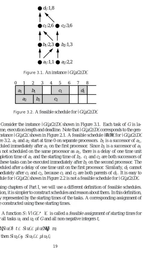
b1:2,3 c1:2,6 c2:3,6 d1:1,8 a1:1,1 a2:2,2 b2:1,3 Figure 3.1.An instance(G,µ,2,D) b2 d1 b1 c1 0 1 2 3 4 5 6 7 a1 a2 c2 8
Figure 3.2.A feasible schedule for(G,µ,2,D)
Example 3.4.2. Consider the instance (G,µ,2,D)shown in Figure 3.1. Each task of G is la-belled with its name, execution length and deadline. Note that(G,µ,2,D)corresponds to the gen-eral scheduling instance(G,µ,2)shown in Figure 2.1. A feasible schedule(σ,π)for(G,µ,2,D)
is shown in Figure 3.2. a1and a2start at time 0 on separate processors. b1is a successor of a1, so it can be scheduled immediately after a1on the first processor. Since b2is a successor of a1 and a2, and b2is not scheduled on the same processor as a1, there is a delay of one time unit between the completion time of a1and the starting time of b2. c1and c2are both successors of b2. Only one of these tasks can be executed immediately after b2on the second processor. The other can be scheduled after a delay of one time unit on the first processor. Similarly, d1cannot be executed immediately after c1and c2, because c1and c2are both parents of d1. It is easy to see that the schedule for(G,µ,2)shown in Figure 2.2 is not a feasible schedule for(G,µ,2,D).
In the remaining chapters of Part I, we will use a different definition of feasible schedules. Using this definition, it is simpler to construct schedules and reason about them. In this definition, a schedule is only represented by the starting times of the tasks. A corresponding assignment of processors can be constructed using these starting times.
Definition 3.4.3. A function S : V(G)→IN is called a feasible assignment of starting times for
(G,µ,m,D)if for all tasks u1and u2of G and all non-negative integers t, 1. |{u∈V(G)|S(u)≤t<S(u) +µ(u)}| ≤m;
3. at most one child of u1starts at time S(u1) +µ(u1); and
4. at most one parent of u1finishes at time S(u1).
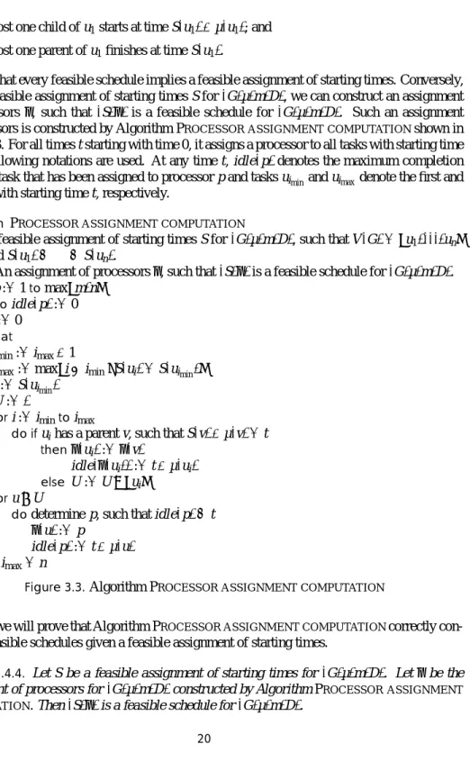
Note that every feasible schedule implies a feasible assignment of starting times. Conversely, given a feasible assignment of starting times S for(G,µ,m,D), we can construct an assignment of processors π, such that(S,π)is a feasible schedule for (G,µ,m,D). Such an assignment of processors is constructed by Algorithm PROCESSOR ASSIGNMENT COMPUTATIONshown in Figure 3.3. For all times t starting with time 0, it assigns a processor to all tasks with starting time t. The following notations are used. At any time t, idle(p)denotes the maximum completion time of a task that has been assigned to processor p and tasks uimin and uimax denote the first and last task with starting time t, respectively.
Algorithm PROCESSOR ASSIGNMENT COMPUTATION
Input. A feasible assignment of starting times S for(G,µ,m,D), such that V(G) ={u1, . . . ,un} and S(u1)≤ ··· ≤S(un).
Output. An assignment of processorsπ, such that(S,π)is a feasible schedule for(G,µ,m,D). 1. forp :=1tomax{m,n}
2. doidle(p):=0 3. imax:=0
4. repeat
5. imin:=imax+1
6. imax:=max{i≥imin|S(ui) =S(uimin)} 7. t :=S(uimin)
8. U :=∅
9. fori :=imintoimax
10. do ifuihas a parent v, such that S(v) +µ(v) =t 11. thenπ(ui):=π(v)
12. idle(π(ui)):=t+µ(ui) 13. elseU :=U∪ {ui}
14. foru∈U
15. dodetermine p, such that idle(p)≤t 16. π(u):=p
17. idle(p):=t+µ(u)
18. untilimax=n
Figure 3.3.Algorithm PROCESSOR ASSIGNMENT COMPUTATION
Now we will prove that Algorithm PROCESSOR ASSIGNMENT COMPUTATIONcorrectly con-structs feasible schedules given a feasible assignment of starting times.
Lemma 3.4.4. Let S be a feasible assignment of starting times for(G,µ,m,D). Letπ be the assignment of processors for(G,µ,m,D)constructed by Algorithm PROCESSOR ASSIGNMENT COMPUTATION. Then(S,π)is a feasible schedule for(G,µ,m,D).
Proof. Because S is a feasible assignment of starting times for(G,µ,m,D), there are at most m tasks u of G, such that S(u)≤t<S(u) +µ(u)for all times t. So for any task u of G, when the tasks of G with starting time S(u)are considered by Algorithm PROCESSOR ASSIGNMENT COMPUTATION, there are sufficiently many processors p, such that idle(p)≤S(u). So every task u has been assigned a processorπ(u). Let u1and u2be two tasks of G. Since S is a feasible
assignment of starting times for(G,µ,m,D), if u1≺Gu2, then S(u2)≥S(u1) +µ(u1). If u2 is
a child of u1andπ(u1)6=π(u2), then S(u1) +µ(u1)=6 S(u2). Otherwise, u2 would have been
assigned to the same processor as u1. Assumeπ(u1) =π(u2). Assume u1has been assigned a
processor before u2. When u2is assigned to a processor, idle(π(u1))≥S(u1) +µ(u1). Because
u2is assigned to processorπ(u2) =π(u1), S(u2)≥idle(π(u1))≥S(u1) +µ(u1). So(S,π)is a
feasible schedule for(G,µ,m,D).
The time complexity of Algorithm PROCESSOR ASSIGNMENT COMPUTATIONcan be deter-mined as follows. Let S be a feasible assignment of starting times. Constructing a list of tasks ordered by non-decreasing starting times takes O(n log n)time. Indices iminand imaxcan be
com-puted by one traversal of the list of tasks ordered by non-decreasing starting times. Since imin
and imaxdo not decrease, updating these indices takes O(n)time in total. For each task u, it has
to be determined whether a parent finishes at time S(u). This takes O(|PredG,0(u)|)time. If there
is a such a parent, then u is assigned to the same processor as this parent. Otherwise, it is added to U and assigned to an arbitrary idle processor. A task is added and removed from U at most once. If U is represented by a queue, then the operations on U take O(n)time in total. If the processors are stored in a balanced search tree ordered by non-decreasing idle(p)-value, then each operation on this tree takes O(log n)time. Soπis constructed in a total of O(n log n+e)
time.
Lemma 3.4.5. For all feasible assignments of starting times S for an instance(G,µ,m,D), Al-gorithm PROCESSOR ASSIGNMENT COMPUTATION constructs an assignment of processorsπ for(G,µ,m,D), such that(S,π)is a feasible schedule for(G,µ,m,D), in O(n log n+e)time.
Because a feasible assignment of starting times for(G,µ,m,D)can be extended to a feasi-ble schedule for(G,µ,m,D), the term feasible schedule will be used for feasible assignments of starting times as well.
Let S be a feasible schedule for an instance(G,m,D). All tasks of G have unit length. For all integers t, define St ={u∈V(G)|S(u) =t}. Then every task in St starts at time t and is completed at time t+1. St will be called the tthtime slot of S. S can be completely represented by a list of time slots: S= (S0, . . . ,S`−1), where`is the length of S. A time slot Stis called idle if it contains less than m tasks.
We conclude this section with a definition that is related to that of feasible schedules.
Definition 3.4.6. Let U be a prefix of a precedence graph G. Let S be a feasible schedule for
(G[U],µ,m,D). Let u be a task in U or a source of G[V(G)\U]. Then u is called ready at time t (with respect to S) if the all predecessors of u are completed at or before time t. u is called available at time t (with respect to S) if
1. u is ready at time t (with respect to S); 2. at most one parent of u finishes at time t; and
3. if a parent v of u finishes at time t, then no child w6=u of v starts at time t.
Let S be a feasible schedule for an instance(G,µ,m,D). It is not difficult to see that any task u is available at time S(u). Note that a task can be available at time t even if m tasks are being executed at that time. Hence any unscheduled task is available one unit of time after the completion time of the last of its predecessors.
3.5
Tardiness
The objective of the scheduling problems studied in the first part of the thesis is the minimisation of the maximum tardiness of a task. Let S be a feasible schedule for an instance(G,µ,m,D). Let u be a task of G. The tardiness of u equals max{0,S(u) +µ(u)−D(u)}; its lateness equals S(u) +µ(u)−D(u). The tardiness of S is the maximum tardiness of a task of G: S has tardiness max{0,maxu∈V(G)(S(u) +µ(u)−D(u))}. If the tardiness of S equals zero, then it is called an in-time schedule for(G,µ,m,D). The lateness of S is the maximum lateness among the tasks of G, it equals maxu∈V(G)(S(u) +µ(u)−D(u)).
S is called a minimum-tardiness schedule for(G,µ,m,D)if there is no feasible schedule for
(G,µ,m,D)whose tardiness is smaller than that of S. Similarly, S is called a minimum-lateness schedule for(G,µ,m,D)if there is no feasible schedule for(G,µ,m,D)whose lateness is smaller than that of S. Because the tardiness of a schedule cannot be negative and an in-time schedule has tardiness zero, any in-time schedule for(G,µ,m,D)is a minimum-tardiness schedule for
(G,µ,m,D). Since the lateness of a schedule can be negative, an in-time schedule for(G,µ,m,D)
need not be a minimum-lateness schedule for(G,µ,m,D).
Clearly, minimising the tardiness and minimising the lateness are closely related problems. Makespan minimisation is also closely related to minimisation of the tardiness: if all deadlines equal zero, then the tardiness of a schedule equals its length. So any algorithm that constructs minimum-tardiness schedules can be used to construct minimum-length schedules.
The tardiness of a schedule can be zero. So for allρ∈IR, such thatρ≥1, aρ-approximation algorithm for tardiness minimisation must construct in-time schedules if such schedules ex-ist. If all deadlines are non-positive, then the tardiness of any schedule is positive, because a non-positive deadline cannot be met. For such instances, aρ-approximation need not construct minimum-tardiness schedules.
However, scheduling with non-positive deadlines is a bit unnatural, because a non-positive deadline cannot be met. There is a model that is equivalent to scheduling with non-positive deadlines: scheduling with delivery times [58, 66]. In this model, every task u has a non-negative delivery time q(u). This is the amount of time that expires after the completion time of u until it is delivered. The objective in scheduling with delivery times is the minimisation of the maximum delivery-completion time (the sum of the completion time and the delivery time of a task). If we have an instance(G,µ,m,D)with non-positive deadlines, then we can choose q(u) =−D(u)
for all tasks u of G. Then minimising the maximum tardiness corresponds to minimising the maximum delivery-completion time.
3.6
Previous results
Scheduling precedence graphs subject to unit-length communication delays is a well-studied problem. Minimisation of the makespan is the most common objective of the algorithms for scheduling with unit-length communication delays. Rayward-Smith [79] was one of the first to study the problem of scheduling precedence-constrained tasks subject to unit-length communi-cation delays. He proved that constructing minimum-length schedules for arbitrary precedence graphs with unit-length tasks is an NP-hard optimisation problem. Lenstra et al. [61] proved the same for scheduling inforests with unit-length tasks. Constructing minimum-length schedules for arbitrary precedence graphs with unit-length tasks on an unrestricted number of processors is an NP-hard optimisation problem as well [47, 77, 80].
For special classes of precedence graphs, it is possible to construct minimum-length sched-ules in polynomial time. Minimum-length schedsched-ules for precedence graphs with unit-length tasks on two processors can be constructed in polynomial time if the precedence constraints form an inforest or an outforest [42, 50, 61, 77, 86] or a series-parallel graph [27]. Varvarigou et al. [86] presented a dynamic-programming algorithm that constructs minimum-length schedules for outforests with unit-length tasks on m processors in O(n2m−2)time; this algorithm constructs minimum-length schedules in polynomial time if the number of processors is a constant. For interval-ordered tasks of unit length, a minimum-length schedule on m processors can be con-structed in polynomial time for any number of processors m [4, 77]. Minimum-length schedules for precedence graphs with arbitrary task lengths on an unrestricted number of processors can be constructed in polynomial time if the precedence constraints form an inforest or an outforest [12], a series-parallel graph [68, 69] or a bipartite precedence graph [77].
In addition, there are many algorithms that approximate the makespan of a minimum-length schedule. Rayward-Smith proved that a list scheduling is a 3−m2-approximation algorithm for scheduling arbitrary precedence graphs with unit-length tasks on m processors. Lawler [59] presented an algorithm that constructs schedules for outforests with unit-length tasks on m pro-cessors; Guinand et al. [41] proved that the schedules constructed by Lawler’s algorithm are at most 12(m−1)time units longer than the length of a minimum-length schedule on m processors. Moreover, Munier and K¨onig [73] use linear programming in their 43-approximation algorithm for scheduling arbitrary precedence graphs with unit-length tasks on an unrestricted number of processors. Munier and Hanen [72] generalised this algorithm to a 73−3m1-approximation algorithm for scheduling arbitrary precedence graphs with unit-length tasks on m processors. Sch¨affter [81] showed how these algorithms can be generalised to a 43-approximation algorithm and a 73-approximation algorithm for scheduling arbitrary precedence graphs with arbitrary task lengths on an unrestricted and a restricted number of processors, respectively.
Two of the few results concerning scheduling problems whose objective is not the minimi-sation of the makespan were presented by M¨ohring et al. [70]; they study scheduling problems whose objective is the minimisation of the weighted sum of completion times. They presented two approximation algorithms: a 103 −3m4-approximation algorithm for scheduling arbitrary
precedence graphs with unit-length tasks on m processors and a 6.14232-approximation algo-rithm for scheduling arbitrary precedence graphs with tasks of arbitrary length on m processors. In addition, there is a 3-approximation algorithm for scheduling series-parallel graphs with unit-length tasks and a 5.80899-approximation algorithm for scheduling series-parallel graphs with arbitrary task lengths [81].
3.7
Outline of the first part
Apart from this chapter, Part I consists of Chapters 4, 5, 6 and 7. These chapters are concerned with the construction of minimum-tardiness schedules in the UCT model. In Chapter 4, an al-gorithm for this problem is presented that consists of two parts. The first part computes smaller deadlines, that are met in all in-time schedules. These deadlines will be called consistent. The second part of the algorithm is a list scheduling algorithm that uses the consistent deadlines to construct a feasible schedule. It will be proved that this algorithm is an approximation algorithm with asymptotic approximation ratio max{2,3−m3}for scheduling arbitrary precedence graphs with non-positive deadlines on m processors and an approximation algorithm with asymptotic approximation ratio 2−m2 for scheduling outforests with non-positive deadlines on m proces-sors. In addition, the algorithm constructs minimum-tardiness schedules for outforests on two processors and on an unrestricted number of processors. Moreover, it is shown that the algorithm is a 2-approximation algorithm for scheduling arbitrary precedence graphs with non-positive deadlines on an unrestricted number of processors.
The least urgent parent property is introduced in Chapter 5. It will be proved that for arbitrary precedence graphs with the least urgent parent property, minimum-tardiness schedules on an unrestricted number of processors can be constructed using a list scheduling approach. The same is proved for scheduling inforests on m processors. If an instance does not have the least urgent parent property, then its deadlines can be increased, such that the resulting instance has the least urgent parent property. The construction of instances with the least urgent parent property is used to construct schedules for arbitrary inforests. Using this construction, we obtain a 2-approximation algorithm for scheduling inforests with non-positive deadlines on m processors.
In Chapter 6, a stronger notion of consistency is introduced by considering pairs of tasks instead of individual tasks. A list scheduling algorithm uses the pairwise consistent deadlines to construct minimum-tardiness schedules for interval orders on m processors and for precedence graphs of width two on two processors. The result on scheduling interval-ordered tasks has been published in the proceedings of ISAAC’96 [89] and a final version will be published in Parallel Computing [93].
In Chapter 7, a dynamic-programming approach is used to construct minimum-tardiness schedules for arbitrary precedence graphs. For precedence graphs of bounded width with unit-length tasks, it constructs minimum-tardiness schedules on m processors in polynomial time. The same is proved for scheduling precedence graphs of bounded width with arbitrary task lengths on an unrestricted number of processors. Moreover, constructing minimum-tardiness schedules for precedence graphs of width three with arbitrary task length on two processors is shown to be an NP-hard optimisation problem.
4
Individual deadlines
The first part of this thesis is concerned with scheduling with non-uniform deadlines subject to unit-length communication delays. Most scheduling problems with precedence constraints and non-uniform deadlines neglect the communication costs. Garey and Johnson [31] were the first that studied a scheduling problem with precedence constraints and non-uniform deadlines. They presented an algorithm that constructs minimum-tardiness schedules for arbitrary precedence graphs with unit-length tasks on two processors. Hanen and Munier [44] showed that this algo-rithm has an asymptotic approximation ratio of 2−2m3 for scheduling arbitrary precedence graphs with unit-length tasks and non-positive deadlines on m processors. In addition, Brucker et al. [11] proved that for inforests with unit-length tasks, minimum-tardiness schedules on m processors can be constructed in polynomial time. Hall and Shmoys [43] showed that list scheduling is a 2-approximation algorithm for scheduling arbitrary precedence graphs with arbitrary task lengths with non-positive deadlines on m processors.
In this chapter, I will present an efficient algorithm that constructs schedules for precedence graphs with non-uniform deadlines subject to unit-length communication delays. The algorithm has the same overall structure as the one presented by Garey and Johnson [31]. The algorithm consists of two parts. The first part computes smaller deadlines that are met in all in-time sched-ules. The deadlines that are met in all in-time schedules will be called consistent. We want these deadlines to be as small as possible. Consistent deadlines will be defined in Section 4.1. The computation of the consistent deadline of a task u depends on the subgraph containing the suc-cessors of u: if u has sufficiently many sucsuc-cessors that have to be completed at or before time d, then the deadline of u is decreased. The algorithm computing consistent deadlines is presented in Section 4.2.
The second part of the algorithm is a list scheduling algorithm that is presented in Section 4.3. This algorithm uses a list ordered by non-decreasing consistent deadlines to assign a starting time to every task. In Section 4.4, the tardiness of the schedules constructed by the list scheduling algorithm will be computed. It will be proved that the algorithm cons