from the National Bureau of Economic Research
Volume Title: NBER Macroeconomics Annual 2001,
Volume 16
Volume Author/Editor: Ben S. Bernanke and Kenneth
Rogoff, editors
Volume Publisher: MIT Press
Volume ISBN: 0-262-02520-5
Volume URL: http://www.nber.org/books/bern02-1
Conference Date: April 20-21, 2001
Publication Date: January 2002
Title: The Cost Channel of Monetary Transmission
Author: Marvin J. Barth III, Valerie A. Ramey
URL: http://www.nber.org/chapters/c11066
FEDERAL RESERVE BOARD OF GOVERNORS; AND UNIVERSITY OF CALIFORNIA, SAN DIEGO, AND NATIONAL BUREAU OF ECONOMIC RESEARCH
The
Cost
Channel
of
Monetary
Transmission
1. Introduction
Traditional economic models posit that changes in monetary policy exert an effect upon the economy through a demand channel of transmission. This view of monetary policy has a long history that has been fraught with debate over whether monetary policy affects real economic variables, and if so, how powerful these effects may be. Much of this research has been devoted to identification of a demand-side transmission mechanism for monetary policy and quantifying its effects. Alternatively, some research- ers have proposed that there may be important supply-side, or cost-side, effects of monetary policy (e.g., Blinder, 1987; Fuerst, 1992; Christiano and Eichenbaum, 1992; Christiano, Eichenbaum, and Evans, 1997; and Farmer, 1984, 1988a, b). One version of this view, which ignores long- run effects, has been called the "Wright Patman effect," after Con- gressman Wright Patman, who argued that raising interest rates to fight inflation was like "throwing gasoline on fire" (1970).
This paper presents aggregate and industry-level evidence that sug- gests that these cost-side theories of monetary policy transmission de-
We wish to thank Wouter den Haan, Charles Evans, Jon Faust, Mark Gertler, Simon Gilchrist, James Hamilton, Alex Kane, Garey Ramey, Matthew Shapiro, Christopher Sims, Chris Woodruff, our colleagues at UCSD and the Board of Governors, as well as partici- pants at UC-Irvine, New York University, the Board of Governors, Rutgers, the San Fran- cisco Federal Reserve, the University of Michigan, the July 2000 NBER Economic Fluctua- tions and Growth Meeting, and the April 2001 NBER Macroeconomics Annual Meeting for useful comments. Christina Romer kindly provided the Greenbook data. Ramey gratefully acknowledges support from a National Science Foundation grant through the National Bureau of Economic Research. The views expressed in this paper are solely the responsibil- ity of the authors and should not be interpreted as reflecting the views of the Board of Governors of the Federal Reserve System. The authors' respective email addresses are marvin.barth@frb.gov and vramey@ucsd.edu.
serve more serious consideration. It is not the purpose of this paper to deny the existence of demand-side effects. Rather, this paper presents evidence implicating supply-side channels as powerful collaborators in the transmission of the real, short-run effects of monetary policy changes. In fact, for many important manufacturing industries, the evidence pre- sented here implies that a cost channel has been the primary mechanism of monetary transmission.
A cost channel of monetary transmission can potentially explain three important empirical puzzles. The first puzzle, noted by Bernanke and Gertler (1995), is the degree of amplification. Empirical evidence sug- gests that monetary policy shocks that induce relatively small and transi- tory movements in open-market interest rates have large and persistent effects on output. Bernanke and Gertler use this result to support their argument that a credit channel working in tandem with the traditional monetary channel better explains the data. A complementary means to explain the observed amplification is to allow monetary policy shocks to have both supply-side and demand-side effects. If this is the case, then a shock to monetary policy could be viewed as shifting both the aggregate supply and aggregate demand curves in the same direction, leading to a large change in output accompanied by a small change in prices.
The response of prices to a monetary contraction is a second empirical puzzle that may be explained by a cost channel. Standard vector auto- regression (VAR) methods suggest that the price level rises in the short run in response to a monetary contraction. This price puzzle was first noted by Sims (1992), and has been confirmed by much subsequent work. It is our view that this may result from short-run, cost-push inflation brought on by an increase in interest rates.
A third puzzle, which we will document shortly, is the differential effect of monetary shocks on key macroeconomic variables when com- pared to other aggregate-demand shifters. Using several measures of aggregate-demand shifters and technology shocks, we show that a mone- tary shock creates economic responses more similar to those due to a technology shock than to an aggregate-demand shock. These results are consistent with our hypothesis that monetary policy shocks affect the short-run productive capacity of the economy.
The literature offers several theoretical foundations for monetary pol- icy as a cost shock. For example, Bernanke and Gertler's (1989) model contains both a demand and a supply component of balance-sheet ef- fects. Several other credit-channel papers suggest that there might be a cost-side channel of monetary policy (e.g., Kashyap, Lamont, and Stein, 1994; Kashyap, Stein, and Wilcox, 1993; and Gertler and Gilchrist, 1994). Most of these papers are empirical, though, and do not explicitly model
the supply-side effects. Nevertheless, the discussion of the results indi- cates the possibility of supply-side effects. Consider, for example, Gertler & Gilchrist's (1994) study of the cyclical properties of small vs. large firms, in which they show that a monetary contraction leads to a decrease in the sales of small firms relative to large firms. The implica- tion is that tight credit is impeding the ability of small firms to produce.1 There are several other examples of general equilibrium macroeco- nomic models that explicitly analyze the supply-side effects of monetary policy through working capital. Blinder (1987), Christiano and Eichen- baum (1992), Christiano, Eichenbaum, and Evans (CEE) (1997), and Farmer (1984, 1988a, b) all begin with the assumption that firms must pay their factors of production before they receive revenues from sales, and must borrow to finance these payments. In most of the models, an increase in the nominal interest rate serves to raise production costs. Thus, a monetary contraction leads to a decline in output through an effect on supply. It is important to note that some type of rigidity is still required for money to be nonneutral. If prices and portfolios adjust immediately, then monetary policy has no initial effect on interest rates, so that neither aggregate demand nor aggregate supply shifts.
The paper proceeds as follows. Section 2 presents aggregate evidence that the effects of monetary policy shocks look more like technology shocks than like demand shocks. Section 3 investigates the importance of working capital in production. Section 4 presents evidence derived from two-digit-level industry data. The results of this analysis show clear indications of the strength of monetary policy as a cost shock at the industry level: many industries display falling output and rising price- wage ratios. Furthermore, the effect appears to be much more pro- nounced during the period from 1959 to 1979. This is also the period in which monetary policy shocks have larger and longer effects on output. Section 5 addresses possible alternative explanations of the empirical results presented in the preceding sections. Finally, Section 6 concludes.
2. A Comparison
of the Effects
of Monetary
Shocks
and
Other Shocks
A useful starting point in an analysis of the supply-side effects of mone- tary policy is a comparison of the responses engendered by identified
1. Some earlier empirical work studied whether rises in interest rates are passed on to prices. Seelig (1974) found small or insignificant effects on markups. Shapiro (1981), on the other hand, estimated a Cobb-Douglas markup equation on aggregate data and found significant interest-rate effects on the price level. To our knowledge, there has been little or no recent empirical work on the subject.
technology and demand shocks on key macroeconomic variables with the responses of those variables to an unexpected monetary contraction. Un- fortunately, the literature is not replete with universally accepted mea- sures of demand and supply shocks.2 Nor is it clear what exactly is meant by "aggregate demand" and "aggregate supply" shocks in a fully speci- fied dynamic general-equilibrium model. Undaunted, we pursue two al- ternative strategies. The first extends work by Shapiro and Watson (1988), Gali (1999), and Francis and Ramey (2001) by using long-run restrictions to identify technology (supply) and other shocks. The second approach uses defense buildups as an example of an exogenous nontechnology (demand) shock. Neither approach is completely uncontroversial, but the similarity of results across the two approaches strengthens our case. 2.1 THE EFFECTS OF SHOCKS IDENTIFIED USING
LONG-RUN RESTRICTIONS
In the first approach, we use a VAR with long-run restrictions to investi- gate the effects of three types of shocks. We follow Gali (1999) in identify- ing technology shocks as the only shocks that have permanent effects on productivity. This assumption is fairly unrestrictive, as it allows for tempo- rary effects of nontechnology shocks on measured productivity through variations in capital utilization and effort. Using a bivariate system with labor productivity and hours, Gali identified two shocks: a technology shock and another shock to labor, which he interpreted as an aggregate demand shock. Interestingly, it is this second shock that appears to drive the business-cycle movements in the economy. Adding nominal variables to the system did not significantly alter his results. Francis and Ramey (2001) present evidence in support of the plausibility of the technology- shock interpretation by investigating the effect of this shock on other key macro variables, such as consumption, investment, and real wages.
We use a combination of variables from the systems estimated by Gali and by Francis and Ramey in order to compare the effects of the various shocks. Consider the following moving-average representation:
Yt = C(L)ut. (1)
Here Yt is a 6 x 1 vector consisting of the log differences of labor produc- tivity (xt), hours (nt), real wages (wt), the price level (Pt), money supply as
2. We were intrigued by Shea's (1993) input-output instruments, but decided against them for the following reason: Of the 26 industries studied, Shea uses residential construction as an instrument for 16 industries, and transportation equipment for 2 industries. If monetary policy is affecting residential investment and motor vehicles at the same time as it is affecting the cost of working capital in upstream industries such as concrete and tires, then output in residential construction or motor vehicles is not a valid demand instrument for the upstream firm.
measured by M2 (m,), and the level of the federal funds rate (ft). The
function C(L) is a polynomial in the lag operator with 6 x 6 matrix coefficients. Shocks to the system, es, e, e, se, et, E f are represented by the vector ut. Note that private output is simply the product of output per hour and total hours.
In order to impose the restriction that no shocks other than e have a
permanent effect on productivity, we require C1' (1) = 0 forj = 2, 3, ..., 6,
where C(1) represents the sum of all moving-average coefficient matri- ces.3 To derive a shock comparable to Gali's aggregate-demand shock, which is the shock to the hours equation, we further impose the restric- tions that C2J(0) = 0 for j = 3, 4, 5, 6. These restrictions essentially put the labor input variable ahead of the other four variables in the ordering. Finally, we require the shock to the federal funds rate to be contempora- neously uncorrelated with the other system variables (except productiv- ity), and, following Beranke and Blinder (1992) and Christiano, Eichen- baum, and Evans (1999), we assume that the shocks to that equation represent monetary policy shocks.
A unit root in productivity is key to identifying the shock. We also assume that hours, real wages, the price level, and the money supply have unit roots, while the federal funds rate is stationary. As Gali shows, the results are not sensitive to changing these auxiliary assumptions. We include four quarterly lags of each variable in the estimation.
To summarize, our goal is to identify three key shocks. The technology shock is found by imposing the long-run restriction that only a technol- ogy shock can have a permanent effect on productivity. The nonmone- tary, nontechnology shock is assumed to be the shock to the hours equation, which Gali has argued behaves most like a demand shock. Fur- thermore, Francis and Ramey have found that while this shock is corre- lated with military dates and oil-shock dates, it is uncorrelated with the Romer dates. Finally, the monetary policy shock is identified as the shock to the federal funds rate. We use quarterly data from January 1959 to March 2000 to estimate the model. The Data Appendix gives complete details about the data used, as well as how the standard errors are calculated. Figure 1 shows the separate effects of a negative technology shock, a negative demand shock, and a contractionary monetary shock on the variables of interest. First note that all three shocks have a negative impact on private output. Both the technology shock and the monetary shock lead to a sustained fall in output. The demand shock, on the other hand, leads to a less persistent fall. All three shocks also lead to falls in hours. Consistent with Gali's original results, hours first rise in response
3. Francis and Ramey show that similar results are obtained with the alternative restric- tions that only set C12 (1) = 0 and Cli (0) = 0 for j = 3, 4, 5, 6.
Figure 1 MONETARY, TECHNOLOGY,
Private Output
AND DEMAND SHOCKS
Private Hours 0.4 0.2 '\ \'""" "- ,,,Technnololgy shock Monetary shock Demand s ck S OCk Demand shock Quarter Productivity _Demand shock Mc fonetary shock ~-~ _ Technology shock 0 4 3 4 8 12 16 Quarter Real Wages Demand shock 0.6 0.4 -0.2 -0.4 -0.8 -o.8 -1. 0.6 0.4 0.2 -0.2 -0.4 -0.6 -0.8
'"Te*~~c~ SMonetary h shock
'
Technology shock 8 1 2 16 20 0 4 8 1 2
Quarter Quarter
Price Level Funds Rate
16 -0.4
-0,6 2o
Quarter Quarter
Line with circles, technology shock; with squares, monetary shock; with triangles, demand shock. Filled marks significant at 10%; open marks significant at 25%.
u11
';~~~~~~~~~~~~~~~~~~~~~~~~~~~~~~~~1 =
to a negative technology shock, but fall immediately in response to the demand shock. The effect of the monetary policy shock on employment is delayed until the third quarter after the shock.
It is in the responses of productivity and real wages that the monetary shock really looks more like a technology shock than like a demand shock. The technology shock and the federal-funds-rate shock both cause a fall in productivity, although the effect is less persistent for the monetary shock, as one would expect for a transitory shock. In contrast, after an initial negative effect for three quarters, the demand shock leads productivity to rise. Thus, the usual explanation given for the decline in labor productivity-a fall in capital utilization-does not appear to apply to declines in hours caused by other demand shocks.
The response patterns for real wages are very similar to those of pro- ductivity, as would be predicted by theory. Both a negative technology and monetary shock lead to declines in real wages, and again, the mone- tary shock is relatively transitory, while the technology shock exhibits more persistence. The responses are consistent with a negative shock to production possibilities that leads to a decline in labor demand. Real wages respond oppositely to a negative demand shock, rising, as would be consistent with a stable production function, and leading to higher labor productivity and hence real wages.
The real-wage results are consistent with several other results from the literature. For example, using a standard recursive VAR, Christiano, Eichenbaum, and Evans (1997) also find that real wages decline in re- sponse to a contractionary monetary shock. Using Shapiro and Watson's (1988) long-run identifying restrictions that aggregate-demand shocks can have no long-run effect on output, Fleischman (2000) finds that aggregate-demand shocks lead to countercyclical movements in real wages. Thus, the response of real wages to monetary shocks is very different from the response to other aggregate-demand shocks.
Figure 1 also shows the effects of the three shocks on the price level and the funds rate. A negative technology shock causes a sustained rise in the price level. A monetary policy shock leads to a temporary increase in the price level, whereas the demand shock does not have much effect. Finally, the funds rate falls in response to a negative demand shock, while it rises in response to a negative technology shock or a monetary contraction (by definition).
A noticeable pattern emerges from the graphs. The response of vari- ables to a monetary policy shock is typically more similar in sign and pattern to a technology shock but is less persistent. Further, as one might expect under a hypothesis that monetary contractions beget both supply and demand effects, the responses to a monetary contraction
generally lie between, or appear to be a mixture of, technology and demand shocks.
2.2 A COMPARISON OF EXOGENOUS MONETARY VS. DEFENSE SHOCKS
As our second line of attack, we present evidence that monetary shocks differ significantly from demand shocks, identified as exogenous de- fense buildups, in their effects on output and real wages. To begin, we present some stark evidence in the form of two graphs of variables in the aircraft and parts industry (SIC 372) from the period 1977 to 1995. Mili- tary spending is an important component of demand for aerospace goods. At the height of the last buildup, the Department of Defense accounted for almost 60% of total shipments from the aircraft and parts industry. Thus, fluctuations in defense spending are an important exoge- nous source of demand variation.
Figure 2a charts real defense spending on aircraft and parts plotted against both industrial production and the real product wage in SIC 372. The real product wage is measured as average hourly earnings in the industry divided by the producer price index for aircraft and parts. The graph plots the logarithms of the data, which have not been detrended or normalized.
From 1977 to 1988, real defense spending on aircraft and parts rose 375%. From 1988 to 1995 it fell by almost the same amount. As Figure 2a clearly demonstrates, the path of defense spending on aircraft has a strong positive correlation with industrial production of aircraft and parts. The correlation is 0.44. In contrast, the real product wage in the industry moves countercyclically. As defense spending rose, real wages plummeted, and as defense spending collapsed, real wages rose; the correlation between the two series is -0.75.
These strongly countercyclical responses to exogenous fluctuations in industry demand are entirely consistent with the effects of a demand shock in a standard neoclassical model with flexible prices. With a stable production function and slow accumulation of capital, an increase in output is necessarily accompanied by a decline in labor productivity and hence a decline in real wages. These patterns are not consistent with a theory of countercyclical markups.
As Ramey and Shapiro (1998) demonstrated more generally, defense spending has similar effects on more aggregate product wages. To high- light the different effects of monetary vs. defense shocks, we compare the impact on real wages and output of a Romer monetary date (Romer and Romer, 1989, 1994) with that of a Ramey-Shapiro military date. In each case, we estimate a system with real wages, output, and the
Figure 2(a) THE EFFECT OF DEFENSE SPENDING ON AIRCRAFT INDUSTRY OUTPUT AND WAGES (QUARTERLY DATA); (b) THE EFFECT OF ROMER DATES AND RAMEY-SHAPIRO MILITARY DATES
Real Wages 25 20 15 10 1977 1980 1985 1990 1995 1977 1980 1985 1990 1995 (a) Real Wages 0.2 0.1 -0.0 -0.1 -0.2 Quarter Quarter (b)
Line with circles, response to a monetary shock; with squares, response to a military shock. Filled marks significant at 10%; open marks significant at 25%.
dummy variable of interest. Eight lags of all variables plus the current value of the dummy variable are included. The comparison is compli- cated by the fact that the Romer dates signal a contraction in output whereas the Ramey-Shapiro dates, which index sudden political events that lead to defense buildups, signal an expansion of output. Leaving aside important potential issues about asymmetry, for comparability we reverse the sign of the Ramey-Shapiro dates to make the shocks in both experiments contractionary.
Figure 2b graphs the response of the logarithm of real GDP and real wages in response to each shock. Although both shocks lead to declines in output, they have opposite impacts on real wages. Defense-induced changes in output are negatively correlated with real wages, while monetary-induced changes in output are positively correlated with real wages.
In contrast with our hypothesis and the evidence presented above, most sticky-price and countercyclical-markup models predict that mone- tary, government spending, and other demand shocks should have simi- lar economic effects. Rotemberg and Woodford (1991), King and Good- friend (1997), and various others have argued that either collusive behavior or sticky prices can lead to countercyclical markups. Since the markup is inversely related to the real wage, countercyclical markups imply procyclical wages. One would expect the effects of defense-spending changes and money-supply changes to have similar but opposite effects on real wages and markups. The results presented here suggest that the transmission mechanism for monetary policy is very different from the transmission mechanism for other nontechnology shocks.
3. The Mechanics
of the Cost Channel
The last section presented qualitative aggregate evidence consistent with a cost channel of monetary policy. We now discuss the quantitative plausibility of the cost-channel hypothesis. The key link in our hypothe- sis is the role of working capital. We argue that just as interest rates and credit conditions affect firms' long-run ability to produce by investing in fixed capital, they can also be expected to alter firms' short-run ability to produce by investing in working capital.
The data support the importance of investment in working capital, whether measured against sales or against fixed capital. One way to measure the magnitude of working capital is to calculate how many months of final sales are held as working capital. Consider the following two measures of working capital: gross working capital, which is equal to the value of inventories plus trade receivables; and net working capital,
which nets out trade payables. On average over the period 1959 to 2000, gross working capital was equal to 17 months of final sales, and net working capital was equal to 11 months of sales.4 Thus, even the smaller net-working-capital measure implies that nearly a year's worth of final sales is tied up in working capital. The level of investment in working capital is in fact comparable to the investment in fixed capital. In manu- facturing and trade, the value of gross working capital equals the value of fixed capital, about $1.5 trillion each.5
There are various ways to incorporate working capital into a model of production. Fuerst (1992), Christiano and Eichenbaum (1992), and CEE (1997) embed a delay between factor payments and sales receipts in their models. They assume that firms must pay workers before selling their goods, so firms must borrow cash from the bank in order to produce. The need to borrow introduces an additional component to the cost of labor. In this setting, the marginal cost of hiring labor is the real wage multiplied by the gross nominal interest rate. In CEE's (1997) version of the model, labor demand is given by
1 W
In N - ( ln(l - a) -In ,L - In Rt - In ), (2)
ca P,
where ac is the coefficient on capital in a Cobb-Douglas production func- tion, ,r is a constant markup, R is the gross nominal interest rate, and W/ P is the real wage.
CEE study a calibrated general equilibrium model in which all of the effects last only one period. They find that the magnitude of the effects on output and labor depends significantly on the labor-supply elasticity. If the labor-supply elasticity is as high as 5, a monetary contraction results in an 83-basis-point rise in the nominal interest rate, a 1.4% decline in hours, and a small rise in prices. It is difficult to find mi- croeconomic evidence in support of such a high elasticity, though. Thus, the cost-channel hypothesis shares the same problem with most eco- nomic models that assume workers remain on their labor-supply curves: a high labor-supply elasticity is essential for matching the quantitative aspects of the data.
Equation (2) is useful for considering the possible magnitude of the direct effects on labor demand of a rise in the nominal interest rate, holding real wages constant. Our evidence on working-capital invest-
4. The inventory and sales data are from the BEA, and the trade credit data are from the
Flow of Funds.
ment suggests that a 1-year lag between paying factors and finally receiv- ing payment is not an unreasonable assumption. Hence, it makes sense to consider an annualized interest rate. If the share of capital is 0.3, then a 100-basis-point increase in the nominal interest rate lowers labor de- mand by 3%, holding real wages constant. The average rise in the fed- eral funds rate during tightening cycles associated with Romer dates is almost 400 basis points. Thus, the direct effects of monetary-induced jumps in the nominal interest rate can have a significant impact on labor demand and output more generally.
The direct effect on the federal funds rate, however, is likely only part of the story. Insights from the credit channel suggest a mechanism by which shocks that initially work through demand may be propagated through the supply side. As demand falls off, firms are faced with accu- mulating inventories and accounts receivable, and falling cash flow. The dropoff in internally generated funds as the stock of working capital rises forces firms to turn to external financing precisely when interest rates are increasing.
The opportunity cost of internal funds increases directly with the fed- eral funds rate, but when firms are forced to turn to external funds, their marginal financing cost typically jumps discretely, due to information asymmetries between the firms and their creditors. In recent quarters, an industrial company rated BBB was usually charged a spread of about 80 basis points over LIBOR on existing lines of credit.6 Since this spread usually rises during periods of tightening credit or during recessions, firms that are forced to renegotiate their lines of credit at such times will face an even greater jump in marginal financing rates. When added to a 400-basis-point increase in the federal funds rate, equation (2) would imply a 15% decline in labor demand with real wages held constant.
The time-lag-in-production model nicely captures several features of the data shown in Figures 1 and 2, but it does not explain how a mone- tary contraction can reduce labor productivity. A model in which work- ing capital has a direct impact on the marginal product of labor can explain such a phenomenon. This can be achieved most directly by including working capital as a factor of production. In fact, there is evidence that this is a valid representation of the role of working capital. Ramey (1989) demonstrates that a model which includes inventories by stage of process as production factors is well supported by the data.
6. Based on data from Loan Pricing Corporation. LIBOR has been the base rate for most firms since the mid-1980s. Prior to that, firms paid a spread over the prime rate, which is typically above a market rate like LIBOR. Hence the above is likely a conservative estimate of the jump in marginal cost of external funding for our data sample.
It is at this point, though, that the cost-channel theory runs into the same problem as the credit-channel theory. Both theories suggest that firms should decrease their inventories and accounts receivable in re- sponse to a monetary contraction. In fact, it is well known that aggregate inventories and accounts receivable rise relative to sales in response to a monetary contraction, at least in the short run (see for example Bernanke and Gertler, 1995, and Ramey, 1992). Some of this rise can be explained by other mechanisms coming into play at the same time. For example, if a monetary contraction also works through product demand, then firms may have unanticipated buildups in final-goods inventories just when they would prefer to hold fewer inventories. Similarly, firms' credit- constrained customers may delay their payments, leading to rises in accounts receivable just when firms need the extra liquidity.
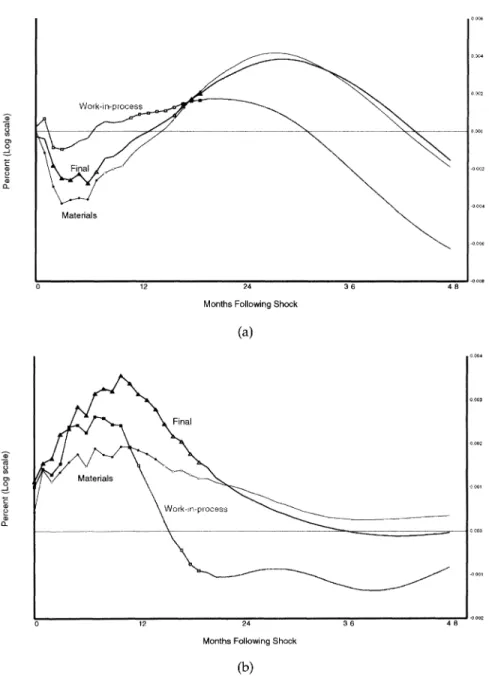
The behavior of the various components of working capital in re- sponse to a monetary contraction is an important part of the story and deserves a much more detailed analysis than we can offer here. We present one piece of suggestive evidence that there may be something to the story. Raw-material and work-in-process inventories are not as sus- ceptible to unintentional buildup. Thus, it is interesting to study what happens to the ratio of inventories by stage of processing relative to labor hours after a monetary contraction.
To measure the effect of a monetary contraction on inventories relative to hours, we use the monthly VAR model that will be presented in the next section.7 We study the response of manufacturing inventories to hours over two different periods of monthly data: January 1959 to Sep- tember 1979 and January 1983 to March 2000. The sample was split for two reasons. First, the new BEA data on real inventories extend back only to 1967. Therefore, we use the old BEA data for the early period and the new BEA data for the second period. Second, as we will demonstrate in the next section, evidence for a cost channel of monetary transmission is much stronger in the pre-Volcker time-series data than in the post- Volcker period.
Figure 3 shows the response of inventories relative to sales for each period. Consider first the period from January 1959 to September 1979 shown in Figure 3a. All types of inventories fall relative to hours in the short run. Interestingly, materials and final goods fall by similar amounts, whereas work in process falls much less. The materials-inventory re- sponse stays negative the longest before becoming positive, at about 13
7. In particular, we estimate equation (3) in which the ratios of materials, work-in-process, and final-goods inventories to hours replace the last two variables in the system.
Figure 3 RESPONSE OF MANUFACTURING INVENTORIES BY STAGE OF PROCESS TO A FEDERAL FUNDS RATE SHOCK: (a) EARLY SAMPLE PERIOD-JANUARY 1959 TO SEPTEMBER 1979; (b) LATE SAMPLE PERIOD-JANUARY 1983 TO MARCH 2000.
00,
Materials
0 12 24 36 48
Months Following Shock
(a)
Wo n Wopc r-k-in-perocess \
0 12 24 36 48
Months Following Shock (b)
Line with circles, materials; with squares, work in process; with triangles, final. Filled marks significant at 10%; open marks significant at 25%.
months. If inventories enhance labor productivity, then this fall in the ratios might help explain the decline in labor productivity.
The behavior of inventories is completely different in the later period, as shown in Figure 3b. In all cases, inventories rise relative to hours. As we shall argue later, the cost channel appears to be much stronger in the early period. These inventory results also support that view.
Finally, we would like to emphasize that we view the cost channel as being only a short-run phenomenon. The evidence for long-run mone- tary neutrality is strong, and we are not suggesting that it does not hold. Figure 1, as well as other figures featured later in the paper, shows that the rise in prices is temporary; the price level does finally end up falling. The cost channel may have a larger effect than the demand channel in the short run because of the nature of the commitments. In the short run, firms cannot find alternative sources for working capital, and may have to cut back dramatically on production. The necessary cutbacks may be amplified because the firm may have commitments to long-term capital investment projects that cannot be cut. As time progresses, firms have more flexibility to reduce investment spending. Bernanke and Gertler's (1995) finding of a delayed effect of a monetary contraction on business fixed investment is consistent with this hypothesis.
4. Industry-Level
Evidence
of Monetary
Policy as a
Supply Shock.
We now explore cross-sectional variation among manufacturing indus- tries for evidence of a cost channel of monetary transmission. There are two motivations for doing so. First, it is interesting to study the extent to which the same patterns we see at the aggregate level also hold at the industry level. Second, if there is heterogeneity in the industry re- sponses, we can determine whether there is a link between the re- sponses and features of the industry that might make the cost channel more important.
The discussion above about the effect of working-capital cost on labor demand easily extends to the industry level. We change the two vari- ables on which we focus, however. First, we use industrial production rather than hours, because of data availability. Since hours and output are so highly correlated, it is doubtful that we will be misled by this change of variables. Second, to facilitate later discussion about the price puzzle and countercyclical markups, it is more convenient to focus on the behavior of the reciprocal of the real product wage, or P/W.
The comovement between P/W and output reveals the nature of the monetary transmission mechanism for particular industries. If a mone-
tary contraction affects an industry primarily through a demand chan- nel, then both industrial production and P/W should fall. (That is, the real product wage should rise.) If a monetary contraction affects an industry primarily by raising its working-capital costs, then falling indus- trial production should be accompanied by rising P/W. Prices should rise relative to wages, because working-capital costs are rising. If both chan- nels are equally strong, we would not expect much movement in P/W.8 4.1 EMPIRICAL FRAMEWORK
We again follow the work of Bernanke and Blinder (1992) and CEE (1999) by identifying monetary shocks as innovations to the federal funds rate (hereafter FFR) after controlling for the Federal Reserve's feedback func- tion. The model features a relatively simple partial identification scheme that allows for control of the price puzzle and flexibility in examining the response of individual time series to monetary policy shocks.
As discussed in the introduction, the price puzzle is the finding that aggregate prices rise in the short run following a monetary contraction identified by the unexplained portion of the FFR. The proposed solu- tion to this puzzle is that the Federal Reserve possesses better informa- tion about coming inflation than is captured in a parsimonious VAR and reacts appropriately. CEE, following Sims (1992), improve their model's information set by including commodity prices as a leading indicator of inflation, to which the Federal Reserve passively responds. CEE demon- strate that this eliminates the price puzzle (note that this is not true in pre-1979 subsamples; see Section 4.3).
Although we have argued that a cost channel could explain this type of behavior of prices, in the interest of conservatism we include two controls for incipient inflation to which the Fed might respond: commodity prices and oil-price-shock dummies. Hoover and Perez (1994) note that identi- fied (negative) monetary policy shifts are highly correlated with oil shocks. We control for the cost effects of oil shocks by including dummy variables in each equation that take the value one during a Hoover-Perez date and zero otherwise.9 Based on Hamilton's (1985) evidence that oil
8. Unfortunately, we cannot use CEE's (1997) study of the response of industry real wages to monetary shocks to assess our hypothesis. They do not compare industry wages with industry price and output. Instead, they examine each industry's wage deflated by a general price deflator.
9. That is, a month identified by Hoover and Perez (1994) as having an exogenous political event that leads to an oil supply shock, based on their reading of Hamilton's (1985) history of postwar oil shocks. Hoover and Perez supplement Hamilton's exogenous political events with the Iraqi invasion of Kuwait in August 1990. Upon the advice of Trevor Reeve, oil economist at the Federal Reserve, we add to this list the election of Hugo Chavez as President of Venezuela in December 1998. Chavez served as the catalyst for OPEC's new-found cohesion in cutting production in early 1999.
price shocks take an average 9 months to induce recessions, we include current and twelve lags of the Hoover-Perez dummies.10
Our equation system consists of two blocks. The macro block features aggregate industrial production, the price level, commodity prices, M2, and the FFR, in that order. The second block consists of two equations for variables of interest, one for industry output and one for the industry price-wage ratio. To achieve more efficient estimation and consistent identification of the FFR shock, the coefficients of the series of interest in the macro-variable equations (including the FFR equation) are con- strained to be zero for each of the industries examined. This is the ap- proach pursued by Davis and Haltiwanger (1997), who point out that this is in essence a pseudo-panel-data VAR. Since the coefficients of the macro-variable equations are fixed across regressions, but the coefficients in the series of interest equations are allowed to vary across industries. To make the above more explicit, consider the following system of seven equations: 12 7 Yt = F' SDt + G;HPt_j + E AkYt-k + Et (3) j=0 k=l where - A,1 O - Pi, t -
Y[ = It, Pt,PCt,M2t,FFRt, Qi, and Ak 5X5 5X2
i,t - 7X7 k k
- 2X5 2x2 -
Here, IPt is industrial production (a proxy for output), Pt is the personal consumption expenditure deflator (a monthly measure of general price levels), PCt is a price index for commodities, M2t is the monthly average of M2, FFRt is the monthly average of the FFR, Qi, is industrial produc- tion in industry i, and Pi, t/W,t is the ratio of price to wage in industry i. In
(3), SDt is a matrix of a constant and seasonal dummies, and HPt is a Hoover-Perez dummy. A is a matrix of endogenous variable coefficients with zero restrictions on the industry variables in the macro-variable equations. Following Bernanke, Gertler, and Watson (1997), we used seven lags.11 All series are in natural-log levels except FFRt. Details on data construction and standard errors are given in the Data Appendix.
10. Hoover and Perez's dummy variable has slightly more explanatory power for industrial production than Hamilton's (1996) net-oil-price-change variable.
We estimated vector autoregressions of this form for total manufactur- ing, durable manufacturing, and nondurable manufacturing, 20 two- digit industries, and one three-digit industry within these categories over three sample periods: the entire period from February 1959 to March 2000, and the two subsample periods from February 1959 to Sep- tember 1979 and from January 1983 to March 2000. Explicitly, we tested the null hypothesis that the change in industry price relative to industry wage is less than or equal to zero following a monetary contraction. We take rejection of this hypothesis as evidence that a cost channel rather than a demand channel is the most important avenue of monetary trans- mission for that industry.
4.2 INDUSTRY RESULTS
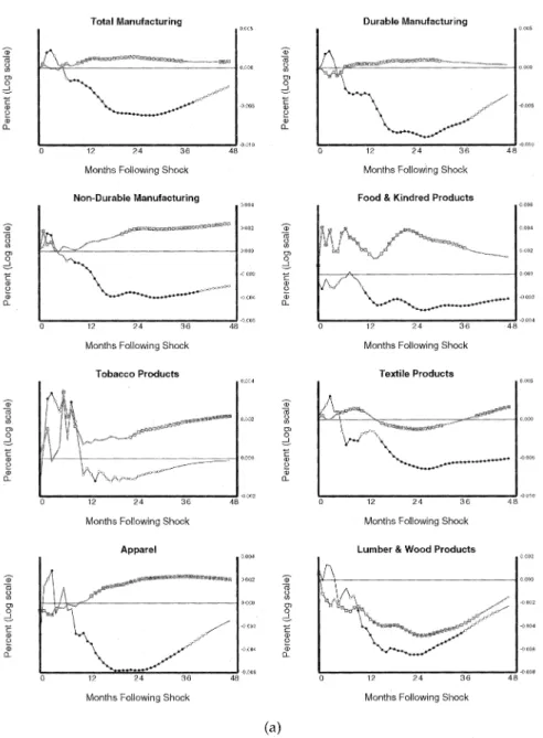
The results are represented in a series of graphs and tables. Figure 4a through 4c show the effect of a positive FFR shock on the price-to-wage ratio and output for the manufacturing aggregates as well as the individ- ual two- and three-digit industries, using our entire data sample for estimation. For 10 of the 21 industries examined and for all three aggre- gates, the impulse response functions show that in response to a posi- tive shock to the FFR, output falls and prices rise relative to wages. The second and third columns in Table 1 summarize the results by describing the behavior of the data during the first 24 months for each industry. The third column presents the results of a test of the null hypothesis that none of the price levels are significantly above zero during the first 24 months. The results clearly reject the null hypothesis at the 10% level for six of the industries analyzed, and we can thus reject the claim that monetary policy exerts its effects solely through a demand channel of transmission. In fact, for important cyclical industries, and even for manufacturing as a whole, the results indicate that monetary policy's primary effects on real variables are transmitted through a supply-side channel.
There is clear evidence of the importance of a demand channel of transmission for eight industries (food, lumber, pulp and paper, chemi- cals, hides and skins, primary metals, fabricated metals, and other dura- bles). Recall, however, the nature of our test: it will only show the presence of a supply channel when its effects clearly dominate those of a demand channel, whose existence we do not deny. That the price re- sponse of lumber exhibits a typical demand-shock pattern does not im- ply that there is not a cost channel of transmission for lumber. The lumber industry too may suffer from a cost channel of transmission, but it is the demand channel whose effects dominate.
If monetary shocks have an effect primarily through increases in costs, however, prices should rise as output falls. This is exactly what we
Figure 4 INDUSTRY OUTPUT & RELATIVE PRICE RESPONSES TO A FEDERAL FUNDS RATE SHOCK: ENTIRE SAMPLE PERIOD: JANUARY 1959 TO MARCH 2000
Total Manufacturing Durable Manufacturing
) 12 24 36
Months Following Shock Non-Durable Manufacturing .- 0.000 ir c 0 -0.002 ? a- -0.004 o a) L -0.006 48 0.002 0.001 " -0.002 -0.004 -0.006 12 24 36 48 Months Following Shock Food & Kindred Products
?0001 , "Il / - 0) 0I (1 a, (1) n -0.001 -0.002 0 12 24 36 48 Months Following Shock
Tobacco Products 0.004 "I 0.002 - >AO I _ m 0 (1 0) 0, Z: 0 12 24 36 48 Months Following Shock
Apparel 0.001 X /--" -0- .ooo0 -0.002 -0.004 0 12 24 36 48
Months Following Shock
~8q~~~~ v -0.002
-0.003
-0.004
0 12 24 36 48 Months Following Shock
Textile Products
000 0.002
0 12 24 36 48 Months Following Shock Lumber & Wood Products
(D (T5 0 0) 0) 0I 1 (1) a, (3 ) 12 24 36 48 Months Following Shock
(a)
Thin line with circles, output: filled, significant at 10%; open, significant at 25%. Thick line with boxes, price/wage: filled, significant at 10%; open, significant at 25%
V,uVV AY
?
J
X\ ...-
"^^"^SHfflBMMtW***"88 * ... I C c I , ( I I ,) 0) o O) -0 v) a) a) a) -E 0 a) I a C: a. 0.002 -0.002 _ -~% ....-.-'Figure 4 CONTINUED
Furniture & Household Durables
0 12 24 36 48 Months Following Shock
Printing & Publishing
_-tb,~"_-
0 12 24 36 4 Months Following Shock Petroleum & Coal Products
,
/'
\1 I \J , 0,004 0.002 Z' I O 000 ) _J a CO f -0.002 - -0.004 -0.006 0.004 -0.002 - Q) 0.002 -0.004 o 0.000 , _ 0.00 a_ 0 12 24 36 48 Months Following ShockHides, Skins, Leather & Related Products 0.004
A 00 0.000 2 a) -0002 0) n000 0 12 24 36 48 Months Following Shock
Pulp, Paper & Allied Products
8-9 ~\
~
---~--- -, 0.000-0.002
-0.006
0 12 24 36 48 Months Following Shock Chemicals & Allied Products
Stv
-0.(
0 12 24 36 41 Months Following Shock Rubber & Plastic Products
A
\ , - 0.000-0.002 -0.006
0 12 24 36 48 Months Following Shock
Stone, Clay & Glass Products 0.002
0.000
-0.002 -0.004 -0.006
0 12 24 36 48
Months Following Shock
(b) cu (n 0) 0 Z:, 1a (1) p 0- Qr 05 U) 0) nn --D (Z CD a) 11- ID CZ E/) 0) -AS I -- - . -. . I n / -0 on / 0.005
"8N1-v...
)10 0.004 0.002 IFigure 4 CONTINUED Primary Metals 0.000 ,- 0) -0.005 ? -0.010 2 Ea 12 24 36 48 Months Following Shock Industrial Machinery & Equipment
12 24 36 4i Months Following Shock
Transportation Equipment
) 12 24 36 41 Months Following Shock Instruments & Related Products
f\ I%\~~~~~~~~ <',~~~~- .. . 0.00
I.A\ ^ ^~^^-0.0'
- 0.0
0 12 24 36 48 Months Following Shock
) 0.000 O o CT -0.005 a v Q_ -0.010 0.005 (1) O.OLS O -0.01 0 Fabricated Metals 0.002 0.000 -0.002 -0,004 -0.006 0 12 24 36 48 Months Following Shock
Electrical Machinery & Equipment o.ooo
0.000
-o.o05
) 12 24 36 40 Months Following Shock Motor Vehicles & Equipment
0 12 24 36 41 Months Following Shock All Other Durable Goods Industries
(0 0 a 0 n - 02 a, nL 3 12 24 36 48
Months Following Shock
(c) Q) _ v 1) n 0 0) v a) - :n 05 0 a 2 a) 8 o Q_ kA ,,,,~~~~~~~~~~~~~~~~~~~~i -0 7\- v.vv -o.D10 c ( ( . ... .,. ... -0.03 0.005 -o.oos 0.002 i 0.0O
AT 10% LEVEL
Whole sample Pre-Volcker Volcker-Greenspan
Industry P/W > 0 Significant P/W > 0 Significant P/W > 0 Significant
Total mfg. 16 3 21 7 6 0 Durables 6 0 18 0 4 0 Nondurables 7 1 23 1 16 0 Food SIC 20 1 0 24 15 18 0 Tobacco SIC 21 0 0 23 2 23 11 Textiles SIC 22 24 8 14 0 0 0 Apparel SIC 23 22 18 15 11 0 0 Lumber SIC 24 0 0 0 0 1 0 Furniture SIC 25 3 0 21 6 7 1
Pulp & paper SIC 26 2 0 19 3 20 0
Printing & publishing SIC 27 0 0 8 0 0 0
Chemicals SIC 28 0 0 15 7 9 0
Petroleum & coal SIC 29 1 0 19 13 16 0
Rubber & plastics SIC 30 0 0 19 14 13 5
Leather SIC 31 0 0 0 0 1 0
Stone, clay, & glass SIC 32 13 0 17 10 18 0
Primary metals SIC 33 0 0 20 17 2 0
Fabricated metals SIC 34 0 0 18 14 6 3
Industrial mach. SIC 35 24 13 17 6 24 0
Electrical mach. SIC 36 24 8 21 0 13 0
Trans. equip. SIC 37 24 20 19 11 6 0
Motor veh. SIC 371 24 20 22 15 14 0
Instruments SIC 38 11 0 14 3 12 0
Other durables SIC 39 0 0 21 0 8 0
Total industries Total industries, n ~ 2 12 6 19 15 10 6 19 15 18 4 16 3 o) .o I?
observe in Figure 4c. Look at the price and output responses of motor vehicles: prices rise steeply and then decay slowly after a peak at 9 months; the output response is nearly the mirror image, falling to a trough at 9 months and slowly increasing from there.
Nor are these unimportant or noninfluential industries showing sig- nificant cost effects of monetary policy. Among those with significant evidence of cost-shock effects are textiles, apparel, industrial machinery, electrical machinery, and transportation equipment. But these results are not limited to the industry level. Total manufacturing exhibits supply- side effects as well. Taken together, this evidence provides a case for a supply-side channel of monetary transmission as a powerful force sup- plementing the often assumed demand channel in creating real effects. Some of the industries that exhibit strong cost-side effects run counter to our prior expectations. One such example is motor vehicles and parts, which shows a very pronounced increase in the ratio of price to wages. One might think that an industry governed by such large firms would not experience large cost effects of a monetary contraction, since they have easy access to commercial paper. A possible explanation is that the primary cost-side effect of a monetary contraction is through changes in market interest rates, rather than bank-loan behavior, so that even large firms experience significant increases in their costs. Another possible explanation is that the small companies that supply parts face loan reduc- tions from their banks.
We now explore the extent to which the effects we identified may have changed over the sample period. To this end, we split the sample into the period February 1959 to September 1979 (the pre-Volcker pe- riod) and January 1983 to March 2000 (the Volcker-Greenspan period). We choose these two subsamples based on the works of Faust (1998) and Gordon and Leeper (1994), who report substantial empirical differ- ences between the aggregate effects of VAR-based identification of mone- tary policy in these two periods. Additionally, the choice of these two subsamples removes the volatility of monetary policy and economic aggregates experienced between late 1979 and 1982 from the data.
Figure 5a through c show the results for the pre-Volcker period. To conserve space we do not show the graphs for the Volcker-Greenspan period. The information for both periods is summarized in columns 4 through 7 of Table 1.
The difference between the two periods is substantial. Overall, we see that the early period through 1979 shows very strong cost-channel ef- fects, whereas the later period shows little evidence of cost-channel effects. In the pre-Volcker period, all three manufacturing aggregates, as well as nearly every industry, exhibit some evidence of a cost-channel
Figure 5 INDUSTRY OUTPUT & RELATIVE PRICE RESPONSES TO A FEDERAL FUNDS RATE SHOCK: EARLY SAMPLE PERIOD: JANUARY 1959 TO SEPTEMBER 1979
Total Manufacturing Durable Manufacturing
12 24 36 Months Following Shock Non-Durable Manufacturing .J'' -~..6 ^?? '-T,M-~:5*'~,'?,<l N' $8 0 12 24 36 48 Months Following Shock
Tobacco Products
0 12 24 36 48 Months Following Shock
Apparel
0 12 24 36 48 Months Following Shock
(0 0 o.ooo o o0 005 0 0,004 0- 0.002 (V ooo oJ o.o0o -0.002 0.004 U) 0,00 0 tD) CL -O 002 - 0.000 CD 0 -0,004 0 12 24 36 48 Months Following Shock Food & Kindred Products
0.006
0.004
.. 002 ~~~~~A o o oo~~~0000
0 12 24 36 48 Months Following Shock
Textile Products
0 12 24 36 48 Months Following Shock Lumber & Wood Products
o~~~~~~~~~~00 0'Fm
0 12 24 36 4 Months Following Shock
(a)
Thin line with circles, output: filled, significant at 10%; open, significant at 25%. Thick line with boxes, price/wage: filled, significant at 10%; open, significant at 25%.
o t) 0 a) o a) ~E g. a) 0. __ a) '3 c 4 I ..'f ' S g ,> M I ^-,>f*- \ C - J \ t..^arSS.,reLA,,s!*3*a^.^a5,^^^^x
\n
v" 0
m1'
atCT
.e1 v* -0002 -0.004 0.005 -0004 -0006 -0.008Figure 5 CONTINUED
Furniture & Household Durables
R. ,-.._^, I? ?~.ft . : .-
PI -
-O.OfO 0 12 24 36 48
Months Following Shock
Printing & Publishing
0.000
< _ ., t0.005
-0.010 0 12 24 36 48
Months Following Shock Petroleum & Coal Products
0.016
r \ ?-0.010
j,: ??L A A A A
12 24 36 Months Following Shock
Pulp, Paper & Allied Products
XI
0 12 24 36
Months Following Shock Chemicals & Allied Products
-e o Ct o a) q) 0- Es ca 0- E:f 48 4 ) 12 24 36 4
Months Following Shock Rubber & Plastic Products
8
8
) 12 24 36 41
Months Following Shock
Stone, Clay & Glass Products
12 24 36 4
Months Following Shock
(b) CZ 0 0) 0 2 - (P c) 0 E a) a) 0i 0 o v E 0 01 0- 12 24 36 41
Months Following Shock
Hides, Skins, Leather & Related Products
V-1- I-O. -\ - I r 'l 0 re, , ' I (D m 0.000 0 O 0) 0) D C- 10 0.005 0.000 0.0
224 * BARTH & RAMEY
Figure 5 CONTINUED
Primary Metals
12 24 36 41 Months Following Shock Industrial Machinery & Equipment
L?:/ . ...
^y>*-^_
) 12 24 36 4r Months Following Shock
Transportation Equipment
) 12 24 36 4 Months Following Shock Instruments & Related Products
.0- y Z B
-O.Ol(
12 24 36 48 Months Following Shock
Fabricated Metals . 005 1 o -o.oo005 0,005 V -O.010 0.005 0 o -0.005 n -0 .o15 0,005 0.005 3 0.005 (D 'a I) 0.000 o - U.0 ) 12 24 36 41 Months Following Shock Electrical Machinery & Equipment
0 12 24 36' 41 Months Following Shock Motor Vehicles & Equipment
:vi
1bN , ._..,
0 12 24 36 41 Months Following Shock All Other Durable Goods Industries
Iy_~__~y,X,5%<Y
N
,@ _,,fi
- 0010
12 24 36 48
Months Following Shock
(c) - a) o (n cI EL a) o Q_ CL ._1 0) d) ?* , Io.oUU -o b ( ( 8 2 0.02 0.01 -0.01 -0.005
A..
price effect. For total manufacturing and for 15 of the individual indus- tries, the price effects are significant at the 10% level. In contrast, only lumber and leather and hides exhibit dominant demand channel effects during this period, and only lumber significantly.
During the Volcker-Greenspan period the cost-channel effects are much weaker. While 16 industries exhibit rising prices, only three do significantly, and the paths of relative prices and output are not as clearly consistent with a supply shock as in the pre-Volcker period.
The results of this section display a good deal of heterogeneity, both across time and across industries. The next two sections will explore whether that heterogeneity can be linked to features that would change the strength of the cost channel.
4.3 INTERPRETING THE TIME PATTERN OF THE RESPONSES
In this section we argue that the changes in the responses we observe over time may be linked with a weakening of the cost-channel mecha- nism in the later period. We discuss institutional changes, and we pro- vide evidence on the changing effect of monetary policy on aggregate variables.
As has been discussed by many observers (e.g., Friedman, 1986), the financial structure of the United States changed significantly during the late 1970s and early 1980s. The private-sector financial innovations begin- ning in the 1970s and the deregulation of the early 1980s led to more efficient and less regionally segmented financial markets. The banking and credit regulations of the earlier period, which limited the scope of lenders and borrowers to respond to sudden monetary contractions, may have allowed monetary policy to restrict the availability of working capital. In the later period, banks and firms had more alternative sources of funds.
A different type of institutional change also occurred over this time period. Romer and Romer (1993) use a narrative approach to show that during the earlier period, contractionary monetary policy was often ac- companied by "credit actions," in which the Federal Reserve sought to limit directly the amount of bank lending. The consequent nonprice rationing led to particularly acute credit crunches, which could have led to severe limitations in working capital.
Finally, the switch from fixed to floating exchange rates during the 1970s may also explain the weakening of the cost channel. With floating exchange rates, a monetary contraction causes the exchange rate to ap- preciate, making imported materials cheaper. Thus, any direct cost-side effects of a monetary contraction may have been counter balanced by the exchange-rate effect in the floating-rate period. Thus, well-documented
differences in financial markets, foreign-exchange markets, and Federal Reserve policy, combined with theory postulating the presence of a cost channel of monetary transmission, may explain the variation we see in the effects of monetary policy through time.