OpenBU http://open.bu.edu
Theses & Dissertations Boston University Theses & Dissertations
2014
Essays on unsecured credit,
uncertainty, and learning
https://hdl.handle.net/2144/15413 Boston University
GRADUATE SCHOOL OF ARTS AND SCIENCES
Dissertation
ESSAYS ON UNSECURED CREDIT, UNCERTAINTY,
AND LEARNING
by
EYNO ROTS
M.A., Boston University, 2013 B.Sc., University of London, 2007
B.Sc., Higher School of Economics, Moscow, 2007
Submitted in partial fulfillment of the requirements for the degree of
Doctor of Philosophy 2014
I would like to thank my advisers Alisdair McKay, Simon Gilchrist, and Francois Gourio for careful guidance, patience, and encouragement. Their contribution to my work is invalu-able. I am also grateful to participants of workshops and seminars at the Department of Economics for useful comments; and to my peers Atanu Bandyopadhyay, Marco Casiraghi, Hyungseok Joo, Sudipto Karmakar, Junghwan Mok, Alejandro Rivera, Kazuta Sakamoto, and Tak-Yueng Wong who have always been kind to offer help and share interesting ideas. I thank Phuong Viet Ngo for tremendous support.
AND LEARNING
(Order No. )
EYNO ROTS
Boston University Graduate School of Arts and Sciences, 2014 Major Professor: Alisdair McKay, Assistant Professor of Economics
ABSTRACT
If lending contracts in an economy take the form of unsecured, non-state-contingent debt, a recession will often be associated with an increase in defaults and a reduction in the supply of credit, which amplifies the contraction. Within this context, I consider the case when the length of an unfolding recession is not immediately obvious; instead, it takes people time to learn about a persistent recession. I apply this scenario to models where the unsecured credit is represented by mortgage loans extended to households and by sovereign debt extended to an emerging economy. I find that in both cases, accounting for uncertainty and learning has a potential to improve the empirical performance of the models.
Chapter 1 explores the U.S. housing market where house prices show a lot of inertia. I develop a general-equilibrium model with the market for housing and mortgages and introduce uncertainty regarding the persistence of business cycles. I show that uncertainty allows the model to better account for the sluggish dynamics of the housing market. In Chapter 2, I use key U.S. macroeconomic data to empirically estimate the structural model developed in Chapter 1. In order to compare the performance of the models with and with-out uncertainty, I use likelihood-based estimation methods. The model with uncertainty proves to be better capable of mimicking the long-lasting changes in house prices and other observable variables.
Chapter 3 contains a theoretical model of a small open emerging economy that looks to refinance its sovereign debt during an unfolding recession of uncertain length. A long
recovery and solvency. Uncertainty about the unfolding scenario adds price risk to long-term bonds and makes them costly to the borrower. Investors’ preferences shift towards short-term bonds which mature before a lot of the uncertainty is resolved and before credit events are likely to happen. Such uncertainty helps explain the empirical fact that emerging economies tend to borrow short term during economic downturns.
1 Learning and the Market for Housing 1 1.1 Introduction . . . 1 1.2 Model . . . 6 1.2.1 Mortgage contracts . . . 6 1.2.2 Households . . . 10 1.2.3 Production . . . 13 1.2.4 Shocks . . . 15 1.2.5 Model Solution . . . 16
1.2.6 Imperfect Knowledge and Learning . . . 17
1.3 Estimation . . . 20
1.3.1 Relating the Model and Data . . . 20
1.3.2 Calibration . . . 21
1.4 Results . . . 24
1.4.1 Maximum-Likelihood Estimation . . . 24
1.4.2 Impulse Responses . . . 27
1.4.3 Unrestricted Kalman gains . . . 33
1.5 Conclusion . . . 37
2 Learning and the Market for Housing: a Likelihood Estimation 39 2.1 Introduction . . . 39
2.2 Methodology . . . 40
2.3 Estimation . . . 43
2.3.1 Calibration and Prior Distributions . . . 43
2.3.2 Posterior Distributions and Posterior Odds . . . 44
2.3.3 Quality of Simulated Samples . . . 49
2.4 Interpreing the Results: Variance Decomposition . . . 50
2.4.2 Historical variance . . . 52
2.5 Conclusion . . . 56
3 Sovereign Debt Maturity in Emerging Economies 57 3.1 Introduction . . . 57 3.2 Model . . . 60 3.2.1 Income Process . . . 60 3.2.2 Bond Prices . . . 62 3.2.3 Policymaker’s Problem . . . 66 3.2.4 Optimal Policy . . . 68 3.3 Results . . . 76 3.3.1 Parameter Specification . . . 76
3.3.2 Results: Baseline Case . . . 78
3.3.3 Lessons from the Model . . . 81
3.4 Final Remarks . . . 90 3.4.1 Future Extensions . . . 90 3.4.2 Conclusion . . . 91 A Supplement to Chapter 1 93 B Supplement to Chapter 2 102 Bibliography 112 Curriculum Vitae 115 viii
1.1 Calibrated parameters . . . 22
1.2 Steady-state performance of the model . . . 24
1.3 Estimated parameters . . . 25
1.4 MLE results for the model with unrestricted Kalman gain . . . 34
2.1 Prior and posterior distributions for the two estimated models . . . 45
3.1 Parameter values of the baseline model . . . 77
1.1 U.S. economy and housing market . . . 2
1.2 Innovation to technology growth rate and learning . . . 19
1.3 Impulse-responses: consumption technology shocks . . . 28
1.4 Impulse-responses: capital technology shocks . . . 30
1.5 Impulse-responses: construction technology and housing supply . . . 32
1.6 Spectral densities of observable variables: model and data . . . 35
1.7 Contribution of technology shocks to house price . . . 36
2.1 Posterior distributions: perfect knowledge . . . 47
2.2 Posterior distributions: imperfect knowledge . . . 48
2.3 Forecast variance decomposition . . . 51
2.4 Historical variance decomposition, imperfect knowledge, panel 1 . . . 53
2.5 Historical variance decomposition, imperfect knowledge, panel 2 . . . 54
3.1 Domain of the first-period value function V1(·) for a given income y1 . . . . 73
3.2 Parameterized and numerically evaluated first-period value function . . . . 74
3.3 Initial-period value function and optimal short-term debt . . . 79
3.4 Effect of Bayesian learning on the optimal policy . . . 82
3.5 Effect of lenders’ and policymaker’s risk-aversion . . . 86
3.6 Effect of persistencesand likelihood pof the persistent income process . . 88
3.7 Effect of initial debtD0 . . . 90
A.1 Impulse responses: redistributional effect of uncertainty . . . 103
B.1 Simulated series: model with perfect knowledge . . . 104
B.2 Simulated series: model with imperfect knowledge . . . 105
B.3 Serial correlation of the series: model with perfect knowledge . . . 106
B.4 Serial correlation of the series: model with imperfect knowledge . . . 107
B.6 Recursive sample means: model with imperfect knowledge . . . 109 B.7 Historical variance decomposition, perfect knowledge, panel 1 . . . 110 B.8 Historical variance decomposition, perfect knowledge, panel 2 . . . 111
LEARNING AND THE MARKET FOR HOUSING
1.1 Introduction
The financial crisis of 2007–2009 has identified the elephant in the room, which is the sheer size of the housing market and its influence on the aggregate economy. Before the crisis, the housing market had been booming for over a decade; rising house prices fueled the lenders’ desire to create new, risky types of mortgages and offer them to the widest set of households, including those with questionable credit history and unreported income. By end of 2006, U.S. households were highly leveraged, with 10 trillion dollars worth of debt, 70% of which was due to mortgages.1 The end of the housing boom forced millions of mortgages into negative home equity, leading to a surge in mortgage foreclosures, massive mortgage write-offs by banks and a collapse of the multi-trillion-dollar market for mortgage-backed securities. The banking sector experienced losses in net worth and a credit crunch. What unfolded was the most severe financial crisis and the longest recession in decades. Events like these require that economic theory provides a better understanding of the housing market.
What is particularly puzzling about the housing market is how slow it is to adjust (see figure 1.1). Following the crisis, the house price index continued to decline steadily for five years;2 and the mortgage foreclosure rate has hovered above the one-percent mark for over three years; more than double its average value for 2002–2005. However, it is common knowledge that market prices should quickly absorb all the information about the current and future state of economy. For example, the S&P500 Index shows that the downward price adjustment in the market for capital lasted for five quarters. To explain this feature
1
Quarterly Report on Household Debt and Credit, Federal Reserve; Mian and Sufi (2009) evaluate the contribution of household leverage to severity of the 2007–2009 recession
2
There was a brief increase in house prices following 2008, when the Federal Reserve announced its large-scale MBS purchase program. The effect of the program on house prices is unclear, though; see Fuster and Willen (2010) for a discussion of the program’s effect on house price.
0.0 2.0 4.0 6.0
1980 1990 2000 2010
GDP components S&P500 Index
1.0 1.5 2.0 2.5
2002 2004 2006 2008 2010 2012 House Price Index
0.0 0.2 0.4 0.6 0.8 1.0 1980 1990 2000 2010
Mortgage Foreclosure starts
0.0 0.5 1.0 1.5 2002 2004 2006 2008 2010 2012 Residential investment Capital investment Aggregate consumption
Figure 1.1: U.S. economy and housing market. All the series are logged and adjusted for inflation; GDP components are per capita. Foreclosure starts are quarterly rates.
of housing market dynamics, I suggest that economic agents did not initially recognize the scope and length of the Great Recession. They observed the deteriorating economy, but did not expect the decline to be persistent. In effect, they were over-optimistic. Households were betting on temporary recession and on a continued housing boom; they were willing to keep purchasing houses and obtaining large mortgages. As the economic downturn continued, the agents eventually realized its scope. Such gradual recognition of a persistent recession can explain the slow reaction of house prices. This mechanism can potentially account for the slow evolution of other variables as well. For example, an unexpected decline in house prices is the major driver of mortgage foreclosures.3
3
The goal of this paper is to study uncertainty about the economic growth as an ex-planation for sluggish dynamics in the market for housing. I take three steps towards this goal. First, I build a dynamic stochastic general equilibrium model with an endogenous market for housing and mortgages that is driven by both transitory and persistent shocks. There is a rich structure of shocks in the model, but I only allow the technology processes to have shocks with different persistence. Technology growth would have two components: a transitory component, or white noise; and a persistent component, an AR(1) process. Second, I consider the situation of imperfect knowledge when economic agents cannot im-mediately recognize the persistence of shocks. They can only observe the aggregate tech-nology growth, but cannot observe its individual components. Using Kalman updating, agents gradually learn about each component’s contribution by observing the evolution of growth through time. And third, I evaluate the ability of the model with such uncertainty to better explain the observed sluggishness in housing-market data. To that end, I look at dynamic features of the model, such as impulse-response functions. I conduct a more thorough likelihood-based empirical estimation for the models with perfect and imperfect knowledge, compare their performance, and present the results in Chapter 2.
There are several arguments to motivate the assumption of imperfect knowledge about the persistence of changes in technology growth. First, it is hard for a model with rational expectations and perfect knowledge to generate any endogenous response of prices to a shock other than a sharp swing followed by gradual recovery back to the steady state. Learning under imperfect knowledge is a powerful tool that may protract the dynamic response of the model variables, as well as improve their co-movement.4
Second, there is empirical evidence to support the assumption of imperfect knowledge and learning, especially about the rate of technological growth. Edge et al. (2007) study the long-run TFP growth rates predicted by professional forecasters5 and find that, despite a plethora of complicated tools used by the professionals, their predictions are strikingly
4
Edge et al. (2007) and Huang et al. (2009) provide similar arguments.
close to a simple learning mechanism based on linear Kalman updating. In addition, Foote et al. (2012) argue that during the Great Recession, mortgage market participants did not know the state of economy; they had beliefs that were ex-post over-optimistic and acted rationally subject to them.
Finally, the assumption of imperfect knowledge about the shocks can help explain why the price adjusts slower in the housing market than in the market for capital. Capital market participants are financial market professionals who closely monitor the state of the economy. The housing market encompasses virtually every household. It is reasonable to believe that participants in the housing market have less knowledge about the state of economy and the future of economic growth, so that they have to rely on learning more.
The novelty of my work is that it combines (i) a market for housing and mortgages with (ii) imperfect knowledge and learning into a model that is (iii) tractable and can be tested directly against the data. The crisis of 2007–2009 has brought the housing market to many economists’ attention, and has motivated the development of models of housing and collateralized household debt. Examples include Chatterjee and Eyigungor (2011), Corbae and Quintin (2013), Garriga and Schlagenhauf (2009), Iacoviello and Pavan (2012), Monacelli (2009), etc. The ability to track house prices, mortgage default rates, loan-to-value ratios, and mortgage risk premiums endogenously in a general equilibrium set-up is a recent achievement of this field that has become possible thanks to an increased interest in the topic. To build a tractable model, I apply the structure of idiosyncratic investment risk developed by Bernanke et al. (1999) to the market for mortgages. In this respect, my work is similar to Forlati and Lambertini (2011).6 Neri and Iacoviello (2008) study the impact of the housing market on aggregate economy. They introduce a rich technology structure that accounts for long-run growth and a portion of short-run fluctuations in house price and residential investment. My model has a similar structure of technology but expands it to incorporate persistent and transitory shocks, as well as imperfect knowledge about
6
The authors develop a dynamic new-Keynesian model to study the shocks originating from the market for mortgages and their impact on the aggregate economy.
them.
The literature on imperfect knowledge and learning has also caught up after the crisis. I employ the learning mechanics similar to Gilchrist and Saito (2006). The authors extend the dynamic new-Keynesian model with financial frictions (Bernanke et al., 1999) to im-plement imperfect knowledge about the persistence of shocks and study its implications for monetary policy. Orphanides and Williams (2007) study the implications of perpetual learning (a rule of thumb based on simple OLS to forecast future prices) for the optimal monetary policy. Eusepi and Preston (2008) show that perpetual learning helps an RBC model amplify and propagate investment and labor supply. Fuster et al. (2010) entertain the finding that agents rely heavily on the recent observations to form their forecasts and show that such assumption helps account for volatility of asset prices and cyclical properties of equity returns in an asset-pricing model.
Given the advances in the literature on housing and the capability of the literature on learning to improve, or, at least, affect model dynamics, it is odd that little has been done to combine the two. One known example is Burnside et al. (2011) who develop a model with heterogeneous beliefs and an intricate learning mechanism. The authors argue that it is difficult to generate protracted house price dynamics in case of homogeneous beliefs because a change in beliefs quickly translates into changes in prices. Their learning mechanism gradually spreads the beliefs like an infection, creating protracted dynamics in house price. I view my work in this respect as an attempt to account for protracted dynamics in house price in a model with homogeneous beliefs, and in a simpler general-equilibrium set-up. In my model, imperfect knowledge and learning make changes in homogeneous beliefs gradual and create sluggishness.
The paper proceeds as follows: section 1.2 defines the model and discusses its key as-sumptions; section 1.3 describes the strategy to evaluate the model empirically; section 1.4 shows the results of empirical estimation; and section 1.5 concludes.
1.2 Model
I design a dynamic stochastic general equilibrium model with endogenous market for mort-gages. Production consists of two sectors: consumption good production and housing con-struction. Households derive utility from both consumption good and housing stock. There are two groups of households: impatient borrowers and patient savers. Borrowers supply fixed labor and earn wage; purchase consumption good and housing stock; and find it opti-mal to use housing stock as collateral to borrow mortgages. Savers purchase consumption good and housing stock; they find it optimal to lend mortgages to the borrowers and invest into capital in both production sectors and earn mortgage interest and capital rent. Savers also supply fixed labor and earn wage. Since the savers originate the capital, they claim all the profit from production if such exists. Time is discreet; one period equals one quarter. The description of the model is more efficient if I explain the workings of the mortgage market first.
1.2.1 Mortgage contracts
To design a tractable market for mortgages with endogenous default rate, loan-to-value ratio, and mortgage premium, I apply the mechanics of endogenous borrowing constraint for entrepreneurs of Bernanke et al. (1999) to mortgages.7
For tractability, I make three simplifying assumptions. First, there are only one-period mortgages available. In reality, mortgages usually have 30-year terms and households at different stages of mortgage amortization behave differently; it is sufficient to mention that households with recently acquired mortgages have a larger outstanding debt compared to the value of the house and are more likely to go underwater and default.8 However, tracking the distribution of households across the stages of mortgage loan repayment would overcomplicate the model. I choose to focus on aggregate behavior of key mortgage market indicators and expect that the model with one-period contracts does not change the results
7This approach is introduced by Forlati and Lambertini (2011). 8
qualitatively. Second, the model features fixed-rate mortgages only: interest rate is known at the time of loan origination. There are adjustable-rate mortgages and contracts with hybrid interest schedules available in the market,9 but the vast majority of mortgages are FRM loans.10 Moreover, for a model with one-period loans, the choice between ARM and FRM contracts is not important, since mortgage interest rates are re-negotiated every period. Finally, the third simplification is that there is no recourse or punishment in case of default. It implies that the household chooses to default on mortgage whenever the value of the house is less than the outstanding debt.
Consider a household agent i that purchases a house Hi,t in period t and pays Hi,tPt
for it, wherePtis the house price in terms of consumption good. To finance this purchase,
the agent can use the house as collateral and obtain a one-period loan Bi,t with a fixed
interest rate ¯rm,i,t. Next period, the outstanding debt is Bi,t(1 + ¯rm,i,t), and the value of
the house isHi,tPt+1Ωt+1(1−δh)ωi,t+1, whereδh is the housing stock depreciation rate and
Ωt+1 is the aggregate shock to the housing stock size. The termωi,t+1 is the idiosyncratic
shock to agenti’s housing stock size that has a log-normal distribution centered at 1:
ωi,t∼F(ω) i.i.d., such that lnωi,t ∼N − 12σω2, σ2ω
⇒E[ωi,t] = 1.
In absence of recourse or punishment, the agent will repay the loan if the value of the house exceeds the outstanding debt:
Hi,tPt+1Ωt+1(1−δh)ωi,t+1 ≥Bi,t(1 + ¯rm,i,t).
For convenience, define the threshold value of idiosyncratic housing stock shock:
¯ ωi,t+1= Bi,t(1 + ¯rm,i,t) Hi,tPt+1(1−δh)Ωt+1 . (1.1) 9
Corbae and Quintin (2013) study the contribution of non-traditional mortgages to the recession.
10
FHFA’s Monthly Interest Rate Survey reports that in 1990–2010, the share of FRM mortgages averaged around 70%.
The household agent will repay the debt if the shock realization is above the threshold next period: ωi,t+1≥ω¯i,t+1.
The most commonly discussed complication of a model with endogenous default is that only a fraction of households default on their loans in equilibrium. To account for it, the model needs heterogeneous households and, as a result, one must explicitly track the endogenous distribution of households in order to compute the default rate and aggregate prices in the economy. This would tremendously complicate the solution of a general equilibrium model, and a convenient approach to this problem is to assume perfect risk-sharing within each household. Let each household be a unit mass of household agents, where each agenticonducts the policy that is optimal for the aggregate household. Then, if a variableZt is a part of the household’s optimal policy, it is true that
Zt= Z 1
0
Zi,tdi, and Zi,t =Zt.
Thus, within each household, agents purchase equally-sized houses and get equivalent mort-gage contracts, so the same threshold ¯ωt+1 is applicable to every agent. Each agent is
subject to agent-specific idiosyncratic shock ωi,t+1, and a fraction of agents will default,
but the household pools the ex-post payoffs from mortgage arrangements and is not sub-ject to idiosyncratic risk. Such set-up renders the model unable to describe potentially interesting effects of mortgage market on household wealth distribution; however, it keeps the solution highly tractable and still retains the essential interplay between the housing purchases, chance of default, and the borrowing constraint. Henceforth, ’household’ stands for a continuum of household agents, and index iis dropped.
The mortgage contract is an arrangement between the saver and the borrower. At period t, the borrower purchases Ht and gets a loan Bt at fixed rate ¯rm,t, so that next
period, her payoff will be
HtPt+1(1−δh)Ωt+1 Z ∞ ¯ ωt+1 ωdF(ω)−Bt(1 + ¯rm,t) Z ∞ ¯ ωt+1 dF(ω).
That is, she only retains the houses and repay the loans of the agents who do not default. In case of a default, the loan is repudiated and the house is lost to the saver, so the payoff is zero. The saver providesBtat periodt, so next period, she will collect
HtPt+1Ωt+1(1−δh) (1−µ) Z ω¯t+1 0 ωdF(ω) +Bt(1 + ¯rm,t) Z ∞ ¯ ωt+1 dF(ω).
Fraction µ captures the cost of default paid by the lender. Foreclosed property is usually sold at a significant discount; there may be legal fees, debt collector’s commission, etc. For such costs, it seems appropriate to assume that they are proportionate to the size of the house.
For brevity of notation, define
Γ(¯ωt) = Z ω¯t 0 ωdF(ω) + ¯ωt Z ∞ ¯ ωt dF(ω), (1.2) G(¯ωt) = Z ω¯t 0 ωdF(ω), (1.3)
where Γ(¯ωt) is the debt repaid to the mortgage lender expressed as the share of the housing
stock collateral, and G(¯ωt) is the average idiosyncratic shock to housing stock associated
with repudiated mortgages. Using equations (1.1)–(1.3) and the fact that E[ω] = 1, the borrower’s payoff becomes
HtPt+1(1−δh)Ωt+1 1−Γ(¯ωt+1), (1.4)
and the saver’s payoff is
HtPt+1(1−δh)Ωt+1 Γ(¯ωt+1)−µG(¯ωt+1).
In effect, a mortgage contract involves two parties co-paying for a house and splitting the value of the house between them upon the mortgage contract settlement: the saver claims Γ(·), the borrower retains 1−Γ(·), andµG(·) is lost due to default. To further the intuition,
let rm,t+1 be the realized saver’s return on mortgage:
Bt(1 +rm,t+1) =HtPt+1(1−δh)Ωt+1 Γ(¯ωt+1)−µG(¯ωt+1) (1.5)
Using (1.5), the borrower’s payoff can be intuitively rewritten as
HtPt+1(1−δh)Ωt+1 1−µG(ωt+1)−Bt(1 +rm,t+1) (1.6)
So, the mortgage arrangement is effectively such that the saver earns the ex-post return rm,t+1 on the loan; while the borrower retains the house, repays the debt at ex-post rate
rm,t+1, and ends up bearing the cost of default.
1.2.2 Households
The total population is fixed at 1; a fraction Ψ are impatient and the remaining 1−Ψ are patient households. The patient household’s discount factor is higher that that of the impatient one: 1>β > β >ˆ 0. (Note that variables and parameters marked with a hat are pertinent to savers; the ones with no accent—to borrowers.) As a result, in equilibrium, the impatient households are borrowers and the patient households are savers.11 Savers provide
borrowers with mortgages and invest into capital; they own the firms in the economy. The infinitely-lived households derive utility from consumption good and housing ser-vices. The lifetime utility function is time-separable and logarithmic:
Ut=
∞
X j=0
βjEtU(Ct+j, Ht+j), where U(Ct, Ht) =νt(lnCt+ψtlnHt);
where ψt is the weight of housing in the utility and νt is the inter-temporal preference
variable. Both ψt and νt are exogenous shock processes. A positive innovation to ψt
corresponds to an increase in housing demand; and a positive innovation to νt makes
11Using the households’ constrained optimization problems, it is straightforward to prove that the
differ-ence in discount factors guarantees that the borrowers find it optimal to borrow and not save, while savers find it optimal to save and not borrow.
households less thrifty, since they value current consumption and housing more compared to their future values, given that the increase in νtis temporary.
Each period, savers maximize the expected utility by choosing the levels of consump-tion ˆCt, housing stock ˆHt, mortgage lending ˆSt, and purchases of capital in consumption
sector ˆKy,t and construction sector ˆKx,t, subject to the budget constraint:
ˆ Ct+ ˆHtPt+ ˆSt+ ˆ Ky,t Ak,t + ˆKx,t = ˆHt−1Pt(1−δh)Ωt+ (1 +rm,t) ˆSt−1+ + (rx,t+ 1−δx) ˆKx,t−1+ Ry,t+ 1−δy Ak,t ! ˆ Ky,t−1+Wt+ ˆΠt. (1.7)
Ak,t is the shock to the cost of consumption-sector capital measured in units of
con-sumption good; this technology process mostly refers to non-tangible capital and is more applicable to consumption good production rather than construction.12 Savers’ wealth in-cludes housing stock retained from the previous period; return on mortgage lending; return on capital investment in both sectors equal to capital rent plus the retained capital stock net of depreciation; wage Wt; and construction-sector profit ˆΠt. As I explain in section
1.2.3, only the construction sector earns non-zero profit. The optimality conditions are the following:
UC,t0ˆ Pt=UH,t0ˆ + ˆβEt h UC,t0ˆ +1(1−δh)Pt+1Ωt+1 i (1.8) UC,t0ˆ = ˆβEt " UC,t0ˆ +1 Ry,t+1+ 1−δy Ak,t+1 !# (1.9) UC,t0ˆ = ˆβEt h UC,t0ˆ +1(rx,t+1+ 1−δx) i (1.10) UC,t0ˆ = ˆβEt h UC,t0ˆ +1(rm,t+1+ 1) i (1.11)
Equation (1.8) is the first-order condition with respect to housing stock: on the left hand, an increment in housing stock would cost some utility due to sacrificed consumption, but on the right hand, the household gains utility because housing stock directly increases utility
12
Neri and Iacoviello (2008) consider this process as well. A more intuitive formulation is ˆKy,t=Ak,tCˆy,t, where ˆCy,tis the amount of consumption good spent on consumption-sector capital.
and because it adds to the next period’s wealth. Euler equations (1.9)–(1.11) predict that mortgage lending and capital investment should all yield the same expected return.
The borrowers choose consumptionCt, housing purchaseHt, and the mortgage contract {Bt,r¯m,t}to maximize the expected utility subject to the constraints:
Ct+HtPt−Bt=Wt+Ht−1Pt(1−δh)Ωt 1−Γ(ωt) (1.12) Bt=EtHtPt+1(1−δh)Ωt+1 Γ(¯ωt+1)−µG(¯ωt+1)/(1 +rm,t+1) (1.13) ¯ ωt= Bt−1(1 + ¯rm,t−1) Ht−1Pt(1−δh)Ωt (1.14)
According to the budget constraint (1.12), the borrower funds her purchases by wage income Wt and mortgage payoffs. The saver’s participation constraint (1.13) and the
definition of the default threshold (1.14) constrain the borrower’s maximization problem: assumably, the borrower knows what implications a mortgage contract {Bt,r¯m,t} has for
the chances of default and that her mortgage repayment must provide the expected return 1 +rm,t+1 required by the saver.
The optimality conditions are the following:
UC,t0 Pt=UH,t0 +βEt h UC,t0 +1Pt+1(1−δh)Ωt+1 1−Γ(ωt+1) i +UC,t0 Et Pt+1(1−δh)Ωt+1 Γ(¯ωt+1)−µG(¯ωt+1) /(1 +rm,t+1) (1.15) βEt h UC,t0 +1Γ0(¯ωt+1) i =UC,t0 Et Γ0(¯ωt+1)−µG0(¯ωt+1)/(1 +rm,t+1) (1.16)
The first-order condition with respect to housing stock (1.15) is similar to that of the saver, except that, apart from direct impact on utility and an increase in next period’s wealth, one more benefit of housing stock for the borrower is that it serves as collateral and increases access to debt (the last term on the right-hand side). Equation (1.16) is the first-order condition with respect to mortgage interest rate ¯rm,t. Recall that the share of
the housing stock claimed by the saver due to the mortgage contract is Γ(¯ω)−µG(¯ω); it is an increasing function of ¯ω (see section A.1.1 of the Appendix). That is,ceteris paribus,
a higher mortgage rate ¯rm,t increases the chance of default and decreases the borrower’s
payoff from mortgage; but, on the other side, the saver will claim a larger fraction of the housing stock, which, in effect, expands the borrower’s capability to get a larger debt.
1.2.3 Production
Consumption good sector employs labor ny,t and capital stock Ky,t−113 to produce the
consumption good Yy,t. There is a technology shock Ay,t that is specific to consumption
good production. The resulting output is Yy,t = (Ay,tny,t)1−αyKy,tαy−1. The sector is
com-petitive and the firms earn zero profit. Profit-maximization gives the standard expressions for wage and capital rent in the sector:
Wy,t= (1−αy)A1 −αy y,t n −αy y,t K αy y,t−1, (1.17) Ry,t=αyA1 −αy y,t n 1−αy y,t K αy−1 y,t−1. (1.18)
The consumption good has three uses: it can be consumed by households, used to purchase capital, and an amountXtof consumption good can be used as an intermediary input for
housing construction: Yy,t=ACt+IKt+Xt.
Construction sector employs labor nx,t, capital stock Kx,t−1, consumption good Xt,
and aggregate housing stock retained from the previous period ¯Ht to produce new housing
stock. Housing construction includes installation of household appliances and furnishing, which motivates the consumption good being a part of housing production function. It also simplifies the derivation of house price and construction sector’s capital rent and wage. As for the retained housing stock, there are two good reasons to make it one of the construction sector’s inputs. First, housing construction, or, more broadly, creation of additional housing stock, includes renovations of the existing houses. And second, inclusion of housing stock in housing construction function adds inertia to it. For an example, a higher level of housing
13I use the time index to indicate the period at which the value of the variable is known. In terms of
timing, consumption good production happens at the beginning of the period, and savers have decided upon the scale of capital investment at the end of the previous period.
construction today would add to the retained housing stock tomorrow and, hence, add to housing construction tomorrow as well, and so on. Effectively, it adds volatility to house prices, since changes in levels of residential investment are more related to swings in the house price rather than the level of housing construction. It is a useful feature of the model if one of its goals is to predict house price movement. In this respect, the retained housing stock is a counterpart for land that is used in similar models with housing sector.14 Finally, there is a technology shock Ax,t specific to housing construction. The resulting output is
the following: Yx,t= (Ax,tnx,t)1−αxk−αxx−αxhKx,tαxk−1X αxx t H¯ αxh t . (1.19)
The retained housing stock is defined simply as
¯ Ht= ΨHt−1+ (1−Ψ) ˆHt−1 (1−δh) Ωt. (1.20)
Construction sector uses the retained housing stock for free—this assumption explains the existence of positive profit from construction sector Πt in equilibrium, which belongs to the savers. This profit is very small, however.15 The profit of the sector is the following:
Πt= (Ax,tnx,t)1−αxk−αxx−αxhKx,tαxk−1XtαxxH¯ αxh
t Pt−Wx,tnx,t−rx,tKx,t−1−Xt. (1.21)
Profit-maximization yields the prices for housing, labor, and capital stock:
Pt= Xt αxx 1 Yx,t , (1.22) Wx,t= Xt αxx 1−αxk−αxx−αxh nx,t , (1.23) rx,t= Xt αxx αxk Kx,t−1 . (1.24)
14Neri and Iacoviello (2008) provide analogous justification for the inclusion of land in housing output
function.
15Rather than having zero housing-sector profit, it is important that housing stock rent does not affect
the decision to purchase housing by the households . Also, the contractors do not pay housing rent when renovating the houses.
Notice that house price is negatively related to all factor inputs except for consumption goodXt. The presence of consumption good as one of the factors of housing construction
allows for easy control of housing supply elasticity. Marginal products of labor and capital also positively depend on consumption good.
The housing sector resource constraint equates household purchases of housing stock net of aggregate housing stock retained from the previous period with the newly-constructed housing:
ΨHt+ (1−Ψ) ˆHt−H¯t=Yx,t. (1.25)
1.2.4 Shocks
Technologies Ay,t,Ax,t, andAk,t are non-stationary stochastic processes defined as
fori∈ {y, x, k}, lnAi,t = lnAi,t−1+γi,t+ui,t, ui,t∼N(0, σ2u,i), i.i.d. (1.26) γi,t = (1−ρi)γi+ρiγi,t−1+vi,t, vi,t ∼N(0, σ2v,i), i.i.d. (1.27)
Technology Ai,t includes a trend component γi,t which is stationary aroundγi and subject
to shock vi,t labeled as persistent shock. The second component of technology growth is
a transitory shock ui,t. Since the technologies are non-stationary, I have to de-trend the
model in order to solve it.16
I consider three non-technological exogenous processes:
lnψt=ρψlnψt−1+ (1−ρψ) lnψ+ψ,t, ψ,t ∼N(0, σψ2), i.i.d. (1.28)
ln Ωt=ρΩln Ωt−1+Ω,t, Ω,t∼N(0, σΩ2), i.i.d. (1.29)
lnνt=ρνlnνt−1+ν,t, ν,t∼N(0, σ2ν), i.i.d. (1.30)
First, ψt is the share of housing stock in household utility. It is a housing demand shock
that shifts household preferences towards housing and affects the house price and the level
of residential investment. Second, Ωt is a shock to aggregate retained housing stock. It
could be viewed as a shock to housing stock depreciation which changes the availability of existing housing. Finally,νtis a shock variable that makes households value current period’s
consumption and housing services differently and affects their inter-temporal choice. The equilibrium is defined dynamically by equations (1.7)–(1.30) and a set of market-clearing conditions: (1−Ψ) ˆSt = ΨBt; Wy,t =Wx,t; ny,t+nx,t = 1; (1−Ψ) ˆKy,t = Ky,t;
(1−Ψ) ˆKx,t=Kx,t; (1−Ψ) ˆΠt= Πt.
1.2.5 Model Solution
Before introducing imperfect knowledge, it is convenient to outline the solution of the model. Because of the technology processes, the model is non-stationary. It can be ap-proximated by the following linear state-space form:
zt= Φ0+ Φ1s1,t+ Φ2s2,t+ Φ3t; (1.31)
s1,t=A1s1,t−1+B1εt; (1.32)
s2,t=s2,t−1+B2εt. (1.33)
In this formulation, zt is the vector of logged observable variables. Vector s1,t represents
the set of log-deviations from the balanced growth path. In other words, the system (1.32) is the de-trended log-linearized version of the model. Vector εt contains all the shocks
to exogenous processes, including the transitory and persistent shocks to technologies: εt= ({j,t}j,{ui,t}i,{vi,t}i)0. Notice that what matters for the de-trended system are not
the levels of technology Ay,t, Ak,t, and Ax,t, but their growth rates. Given i ∈ {y, k, x},
I redefine equations (1.26) and (1.27) in terms of log-deviations from the steady-state growth rates in order to include them in the system (1.32):
˜
gi,t = ˜γi,t+ui,t; (1.34)
˜
where gi,t = Ai,t/Ai,t−1 is the growth rate, so that ˜gi,t = lnAi,t −lnAi,t−1 −γi is the
log-deviation of the growth rate from its steady state; and ˜γi,t =γi,t−γi is the deviation
of the growth rate’s persistent component. Consequently, the state vector s1,t contains
these variables: s1,t = (. . . ,{g˜i,t}i,{γ˜i,t}i)0. Note that s1,t is stationary, which justifies
the use of log-linearization for this component of the model. Vector Φ0 captures the steady-state values of the de-trended observable variables. The last two terms capture the non-stationary stochastic and deterministic components of technology processes. In the Appendix, section A.1.2 explains the de-trending procedure; section A.1.3 provides the complete de-trended system; section A.1.4 provides its log-linearized version correspondent to equation (1.32); and section A.1.6 explains how different components of the system (1.31) capture the technology processes.
1.2.6 Imperfect Knowledge and Learning
The model with perfect knowledge implies that agents can perfectly observe both persistent and transitory innovations to exogenous processes. In case of imperfect knowledge, agents only observe the total level of productivity—or, equivalently, its growth rate—but the shocks ui,t and vi,t and the persistent component γi,t are unobservable. For an example,
the agents can observe a large increase in technologyAi,t but cannot immediately tell if the
higher growth is due to the persistent componentvi,t and, thus, if the growth rate will be
higher in the future as well; or if it is a one-period increase due to the transitory component ui,t. To resolve this uncertainty, the agents have to wait and observe the growth rate for
several periods in order to gradually learn about the nature of the shock. I assume that the agents use a simple linear steady-state Kalman filter for this purpose. The motivation behind the steady-state filter is that the agents have observed a long history of productivity in the economy and have an idea about the transitory and persistent shocks, their volatility and persistence. For a technologyAi,t, the agents are assumed to know the values σvi,σui, ρi, andγi. An interesting question (which I address in section 1.4.3) is whether the values
truth—but the point is that the agents are assumed to rely on their belief and implement the steady-state filter.
Define ˆγ˜i,t = E(˜γi,t|g˜i,0, . . . ,˜gi,t) as the inferred value of the technological growth’s
persistent component at time t given all available observations of the growth rate up to period t. Then, given the equations (1.34) and (1.35), the standard result is the following Kalman-updating equation:17
ˆ ˜
γi,t =λig˜i,t+ (1−λi)ρiγˆ˜i,t−1.
This expression summarizes the way households learn about the value of persistent com-ponent of technological growth by means of the steady-state Kalman filter. Parameter λi
is the steady-state Kalman gain:
λi = di−(1−ρ2i) + q (1−ρ2 i)2+d2i + 2(1 +ρ2i)di 2 +di−(1−ρ2i) + q (1−ρ2 i)2+d2i + 2(1 +ρ2i)di , (1.36)
wheredi=σ2v,i/σ2u,irelates the volatilities of persistent and transitory shocks. The Kalman
gain positively depends on di and ρi. Intuitively, if the persistent shock is more volatile
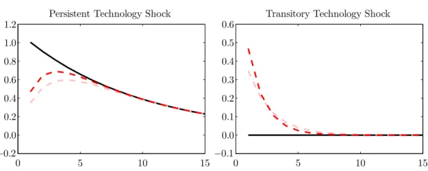
compared to the transitory shock or if the persistent component has a higher autocorrela-tion coefficient, the agents infer that a sequence of higher growth rates is more likely to be the result of a shock to persistent component rather than a sequence of transitory shocks. Figure 1.2.6 demonstrates the process of learning. There is a shock to technology that increases the growth rate gi,t. The graph on the left shows the case of persistent shock.
Initially, the agents do not completely realize that the shock is persistent (there is a chance that it is a transitory shock), so the inferred value of the persistent component is lower than the actual value. As agents keep observing the evolution of the growth rate, they gradually learn that the shock has been persistent, since the observed path of the growth rate is far more likely to be the result of one persistent shock rather than a series of transitory
17
Persistent Technology Shock −0.2 0.0 0.2 0.4 0.6 0.8 1.0 1.2 0 5 10 15
Transitory Technology Shock
−0.1 0.0 0.1 0.2 0.3 0.4 0.5 0.6 0 5 10 15
Figure 1.2: Impulse-responses: innovation to technology growth rate. Evolution of the persistent technology growth component ˜γi,t due to one-percent positive persistent and
transitory shock (vi,tandui,t, respectively). The solid black lines show the actual responses
of the variable. The dashed lines show the inference about this unobservable variable implied by Kalman filtering. The dark dashed lines are for σ2iv/σ2iu = 0.5, and the light dashed lines are forσ2
iv/σ2iu= 0.25. Autoregressive coefficient for the persistent component
is set atρi = 0.9.
shocks. The two lines eventually converge. A relatively higher variance of transitory shock (low di) corresponds to slower learning, since a sequence of positive transitory shocks that
can explain the observed growth rate path becomes more likely. On the right-side graph, the shock is to the transitory component, and the learning mechanics are analogous. The persistent component does not change, but initially, agents realize that the shock might be persistent. After observing zero growth rates in all subsequent periods, the agents eventually learn that the shock is transitory.
In order to impose the case of imperfect knowledge on the model, I take the linear system (1.32) and replace the actual values of persistent technology components and shocks to tech-nologies with the ones inferred through Kalman filtering, so that the state vector becomes ˆ
s1,t = (. . . ,{g˜i,t}i,{γˆ˜i,t}i)0 and the vector of shocks becomes ˆεt = ({j,t}j,{uˆi,t}i,{vˆi,t}i)0.
Furthermore, for each of the technology processes, I add a set of equations that relate the Kalman-filtered estimates and the actual values of components of technology processes:
ˆ
ˆ
ut= (1−λi)(˜γi,t+ui,t)−(1−λi)ρiγˆ˜i,t−1;
˜
γi,t=ρiγ˜i,t−1+vt.
1.3 Estimation
The empirical exercise outlined below seeks to establish how technological shocks contribute to the observable data pertinent to aggregate economy and to the market for housing in particular, and how the assumption of imperfect knowledge affects this contribution. For this purpose, I perform the classical maximum likelihood estimation of the model under both perfect and imperfect knowledge. The parameters estimated by means of MLE are all the parameters describing the exogenous processes (shock variances, autoregressive coefficients, steady-state technological growth rates); all the other parameters are calibrated so that the steady state of the model matches certain empirical targets. Given the observed data ZT = {zt}Tt=1 and a parametrization θ, I can compute the log-likelihood function
l(ZT|θ) = ln ΠTt=1Pr(zt|Zt−1, θ) by means of sequential Kalman filtering. In order to find
the vector of parametersθ∗Mthat maximizes the log-likelihood function for the models with perfect and imperfect knowledgeM ∈ {P,I}, I use a combination of Newton methods.18
1.3.1 Relating the Model and Data
The aggregate resource constraint is a combination of the borrower’s and saver’s budget constraints (1.12) and (1.7): ΨCt+ (1−Ψ) ˆCt | {z } Household consumption +Ky,t Ay,t −(1−δy) Ky,t−1 Ay,t−1 +Kx,t−(1−δx)Kx,t−1 | {z } Non-residential investment + 18
I start the search for the parameter vectorθ∗Musing my own version of the BFGS routine; then, I use Chris Sims’ optimization algorithm (http://sims.princeton.edu/yftp/optimize/) to ’polish’ the result.
ΨHt−1Pt(1−δh)µE[ω|ω <ω¯t] | {z } Cost of default +Pt(ΨHt+ (1−Ψ) ˆHt−H¯t) | {z } Residential investment =Yt+Yx,tPt | {z } GDP (1.37)
This equation conveniently relates the model to the four key variables taken from the data: aggregate consumption ACt, which is the sum of household consumption and the cost
of default; non-residential investment IKt; and residential investment IHt. The fourth
observable variable is the house price, Pt. The data set includes the four quarterly series ZT = {ACt, IKt, IHt, Pt}Tt=1 and spans 1975–2013. The full description of the data is
provided in section A.2 of the Appendix.
1.3.2 Calibration
The vector of parameters θ that is estimated by MLE describes the exogenous processes: θ={ρi, γi, σi}. I calibrate the rest of the parameters to match the steady state of the model
with a corresponding number of empirical targets.19 Table 1.1 summarizes the calibration. Saver’s discount factor is set to match the quarterly interest rate, which corresponds to the real expected return on capital in my model. For 1975–2006, I have estimated the average quarterly 3-Month Treasury Bill rate adjusted for expected inflation to be 0.5%.20 Data show that the equity risk-premium over the T-Bills was 1.7% in quarterly terms for the same period;21 and, for 30-year corporate bonds rated Aaa by Moody’s, the
risk-premium over the Treasury bonds with the same maturity was 0.2%.22 These values imply a reasonable range for the real interest rate between 0.7% and 2.2% per quarter. I set ˆβ = 0.9888 to match the target of 1.5%. Given ˆβ, the borrower’s discount factor β, cost of default parameter µ, and variance of idiosyncratic housing stock shock σω are
19
The technology growth ratesγi, i∈ {y, k, x}obtained via MLE affect the steady state of the model, which slightly complicates the calibration. However, they are quite insensitive to calibration, so I use the growth rates obtained after a few initial MLE runs to calibrate the other parameters.
20
Inflation is the growth in CPI for All Urban Consumers: All items less shelter (BLS). Expected inflation is the OLS prediction of the quarterly inflation rate based on four lagged values.
21
Ibbotson Risk Premia Over Time Report, 2013
Table 1.1: Calibrated parameters
Parameter Value Meaning
ˆ
β 0.9888 Saver’s discount factor
ψ 0.17 Share of housing in utility function
αy 0.25 Share of capital in consumption good production αxk 0.1 Share of capital in housing construction
αxh 0.1 Share of housing stock in housing construction αxx 0.1 Share of consumption good in housing construction δy 0.02 Depreciation rate of consumption capital
δx 0.025 Depreciation rate of housing construction capital δh 0.015 Depreciation rate of housing stock
N 1.0 Population size
Ψ 0.6418 Borrowers’ share in population
β 0.9587 Borrower’s discount factor
σω 0.1902 Standard error of idiosyncratic shock to house size
µ 0.1172 Cost of mortgage foreclosure
chosen jointly to match the loan-to-value ratio, default rate, and mortgage premium. The annual mortgage premium is chosen to be 1.5% based on the average 30-year mortgage premium over the 30-year Treasury bonds for 1977–2006.23 Following the literature, the target default rate is chosen to be 2%, which is the average delinquency rate for residential estate loans for the decade preceding 2007, according to the Federal Reserve. Neri and Iacoviello (2008) report the average loan-to-value ratio to be 76% between the years 1973 and 2006.24 At the rate of default of 2%, such high loan-to-value ratio would correspond to an extremely low borrower’s discount factor. I set a more moderate target of 65%. The resulting values ofµ andσ are in line with the literature;25 the borrower’s discount factor is quite low, which is to say that the model implies a very impatient borrower in order for her to accept the mortgage that has a high chance of costly default.
Capital depreciation in consumption good sector is set at δy = 0.02. Together with
23Ibid. 24
Finance Board’s Monthly Survey of Rates and Terms on Conventional Single-Family Non-farm Mort-gage Loans (table 19)
25
Forlati and Lambertini (2011) set σ = 0.2 and µ = 0.12. The cost of debt parameter µ is quite conservative; for a detailed discussion of foreclosure discounts, see Campbell et al. (2009).
capital share in consumption good production function, it helps to set the share of non-residential investment in GDP. Housing sector capital stock is relatively too small for it to have a significant impact on the aggregate investment share. Housing sector capital depreciation is set at δh = 0.025 to reflect the fact that capital stock has shorter life in
construction sector. The share of capital is set at αy = 0.25 in consumption good sector
and αxk = 0.1 in construction sector, which is less capital-intensive. These shares are
considerably lower than the conventional one third due to the definition of GDP which only includes private consumption and private fixed investment. Davis and Heathcote (2005) use the NIPA Input-Output tables to estimate the share of capital to be 0.13 in construction, 0.24 in services, and 0.31 in manufacturing. The shares of consumption good and housing stock in construction output are chosen to be αxx = 0.1, αxh = 0.1. These
parameter values are according to Davis and Heathcote (2005), which set these shares for consumption good and land. I am using the empirically estimated share of land to measure the contribution of housing stock because housing stock used in construction acts as a counterpart to land in my model.26
The share of housing in the utility is set in combination with housing depreciation rate to match the share of residential investment in GDP and the ratio of housing stock value to GDP:ψ= 0.17, δh= 0.01. The share of borrowers in total population equals the share
of homeowners that had mortgages in 2006:27 Ψ = 0.6418.
Table 1.2 shows that the steady-state of the model is close to the empirical targets that I have set. Given the calibration, I estimate the remaining parametersθ={γi, ρi, σi} via
the maximum-likelihood estimation.
26
See section 1.2.3 for details
Table 1.2: Steady-state performance of the model
Measure Model Target Target source
Quarterly interest rate, % 1.51 1.50 Data, Federal Reserve
IK/GDP, % 13.60 15.00 Data, BEA
IH/GDP, % 6.14 6.00 Data, BEA
p×H/GDP 1.14 1.36 Neri and Iacoviello (2008)
K/GDP, non-residential 2.31 2.05 Neri and Iacoviello (2008)
K/GDP, residential 0.04 0.04 Neri and Iacoviello (2008)
Annual mortgage premium, % 1.50 1.50 Data, Federal Reserve Mortgage default rate, % 2.00 2.00 Data, Federal Reserve
Loan-to-value ratio, % 64.60 65.00 Data, FHFA
1.4 Results
1.4.1 Maximum-Likelihood Estimation 1.4.1.1 Parameter estimates
Table 1.3 presents the parameter estimates with associated standard errors28for the cases of perfect and imperfect knowledge. While the shock variances do not describe their rel-ative importance, the table reveals a few notable facts. First, the processes for which ambiguity about the persistence of technology shocks matters are capital and consumption technologies. Under imperfect knowledge, these are the only processes with both persistent and transitory shocks significant. At the same time, agents always know that the transi-tory component is driving the construction technology because the persistent component is nonexistent. Second, capital technology shocks have significant variances only under imperfect knowledge. Third, imperfect knowledge makes both transitory and persistent components of consumption technology significant, while perfect knowledge renders the transitory shock insignificant. I look into the reasons behind these facts below.
In both cases, housing demand shockψtis insignificant. Retained housing supply shock
28
Standard errors are evaluated using delta-method and the Hessian that is numerically estimated for the likelihood function.
Table 1.3: Estimated parameters Case I: Imperfect Knowledge
Technological shocks γi ρi σui σei Consumption production (gy) 0.0069 0.4945 0.0054 0.0054 (0.0009) (0.0725) (0.0009) (0.0009) Capital creation (gk) -0.0095 0.8916 0.0123 0.0022 (0.0015) (0.0401) (0.0031) (0.0003) Construction (gx) -0.0032 0.9900 0.0199 0.0000 (0.0016) (x.xxxx)† (0.0012) (0.0000) Non-technological shocks ρi σi Inter-temporal preference (ν) 0.9900 0.0000 (x.xxxx)† (0.0000) Housing demand (ψ) 0.9900 0.0000 (x.xxxx)† (0.0000)
Retained housing supply (Ω) 0.0000 0.0184
(0.0000) (0.0011)
Case II: Perfect Knowledge
Technological shocks γi ρi σui σei Consumption production (gy) 0.0060 0.3791 0.0000 0.0074 (0.0009) (0.0328) (0.0000) (0.0005) Capital creation (gk) -0.0079 0.3579 0.0000 0.0000 (0.0014) (0.4741) (0.0000) (0.0000) Construction (gx) -0.0099 0.9900 0.0204 0.0007 (0.0016) (x.xxxx)† (0.0012) (0.0001) Non-technological shocks ρi σi Inter-temporal preference (ν) 0.9900 0.0236 (x.xxxx)† (0.0026) Housing demand (ψ) 0.9900 0.0000 (x.xxxx)† (0.0000)
Retained housing supply (Ω) 0.2832 0.0105
(0.0505) (0.0014)
† The values of autoregressive coefficient were restricted to not exceed 0.99—this
re-striction is only effective for the housing construction technology and inter-temporal preference in case of perfect knowledge.
Ωtis either a white noise or a very nonpersistent process. Inter-temporal preference shock νt is only significant under perfect knowledge. It seems that the contribution of capital
technology shock is replaced by that of the inter-temporal preference shock under perfect knowledge; both shocks affect the saver’s decision to invest. Inter-temporal preference shock is estimated to be extremely persistent; I put a cap ofρν = 0.99 on its autoregressive
coefficient. Wen (2006) explains that a positive shock to inter-temporal preference variable, when it is transitory, makes households value current utility relatively much more, so they prefer to consume more and reduce investment; the result is that consumption and investment are negatively related. A more persistent shock also increases the value of future utility by more and allows for better co-movement between consumption and investment.
1.4.1.2 A Note on Comparative performance
The model with imperfect knowledge (I) performs better in terms of likelihood: the achieved log-likelihood is l(ZT|θ∗I,I) = 1637.9; for the case of perfect knowledge (P),
the value is l(ZT|θP∗,P) = 1617.9, where θ∗ is the vector of parameters that maximizes
the likelihood function. While this is a considerable difference for log-likelihood values, the two numbers are not directly comparable, since the two models have different struc-tures and do not simply correspond to two alternative parameter specifications. A more appropriate way to compare the two models would be to specify a prior over the parameter space p(θ|M) for the two models of perfect and imperfect knowledge M ∈ {P,I}and use numerical methods to compute the marginal likelihood p(ZT|M) = Rp(ZT|θ)p(θ|M)dθ.
Then, it is straightforward to compare the two models in terms of posterior odds in favor of the model with imperfect knowledge:
P O= p(ZT|I) p(ZT|P) .
1.4.2 Impulse Responses
The goal of this subsection is to shed light on how imperfect knowledge affects the dynamics of the model. I limit the discussion to responses to shocks that are significant under imperfect knowledge.
1.4.2.1 Consumption technology shocks
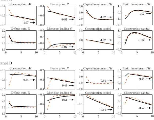
Panel A of figure 1.3 shows impulse responses of key variables due to a negative one-standard-deviation shock to persistent component of consumption technology growth gy,t.
Consumption good is used to pay for capital and new housing stock, so a less productive consumption good sector results in lower consumption and investment, which all eventually stabilize at 1.07 percent below the pre-shock balanced growth path. Construction capital stock initially increases because construction sector becomes relatively more productive, but eventually, scarcer consumption good makes construction capital stock fall. Because consumption sector becomes relatively less productive than construction, housing demand declines together with house prices, leading to a higher mortgage default rate and lower mortgage lending. Notice how imperfect knowledge delays the responses: initially, people believe in quick recovery, so consumption, housing demand, and house prices remain higher; these variables adjust as households gradually recognize the persistent shock.
Overall, imperfect knowledge delays the responses of house price, consumption, and mortgage default rate. This is the kind of protraction which Burnside et al. (2011) argue to be hard to achieve when the household beliefs are homogeneous. In part, they prove to be right: this protraction is very limited under the estimated parametrization, and the responses for the two models converge after 2–3 quarters. Kalman gains are defined by parameters of technology processes according to equation (1.36), and consumption tech-nology process is such that agents learn about the nature of the shock very quickly. Still, the persistent shock has an ability to explain a lot of longer-term dynamics in observable variables, since its contribution builds up over time while the immediate impact is subdued.
Panel A -1.07 Consumption,AC −0.8 −0.6 −0.4 -0.83 House price,P −0.8 −0.6 −0.4 -1.07 Capital investment,IK −4.0 −2.0 0.0 2.0 -1.07 Resid. investment,IH −2.0 −1.0 0.0 1.0 Default rate, % 1.9 2.0 2.1 2.2 0 5 10 -1.07 Mortgage lendingS −0.9 −0.8 −0.7 −0.6 0 5 10 -1.07 Consumption capital −0.5 0.0 0.5 0 5 10 -1.07 Construction capital −0.5 0.0 0.5 1.0 0 5 10 -1.07 -1.07 -1.07 -1.07 -0.83 -1.07 -1.07 Panel B -0.54 Consumption,AC −0.5 −0.4 −0.3 -0.42 House price,P −0.4 −0.3 −0.2 -0.54 Capital investment,IK −2.0 −1.0 0.0 1.0 -0.54 Resid. investment,IH −1.0 −0.5 0.0 0.5 Default rate, % 1.9 2.0 2.1 2.2 0 5 10 -0.54 Mortgage lendingS −0.8 −0.6 −0.4 0 5 10 -0.54 Consumption capital −0.2 −0.1 0.0 0 5 10 -0.54 Construction capital −0.3 0.0 0.3 0.6 0 5 10 -0.54 -0.54 -0.54 -0.54 -0.42 -0.54 -0.54
Figure 1.3: Impulse-responses. Panel A: persistent consumption technology shock, vy.
Panel B: transitory consumption technology shock, uy. Percentage deviations of
non-detrended variables from the balanced growth path due to one-standard-deviation negative shock. Solid lines represent the case of certainty; dashed lines represent uncertainty. For default rate, the values are absolute, compared with their steady-state values (dotted lines). Numbers near the arrows show where the deviations will stabilize after 400 quarters.
Notably, imperfect knowledge creates additional redistribution of wealth between bor-rowers and savers during a recession. Immediately after the persistent shock, borbor-rowers are too optimistic about the future house price and bet on it by obtaining large mortgages and making large housing purchases. These decisions turn out to be bad ex post: in the periods following the shock, unexpectedly low house price results in higher default rate and reduces the borrowers’ net worth, consumption, and housing demand. Meanwhile, savers are able to purchase cheaper housing stock and use the extra savings to maintain higher consumption. Section A.3 of the Appendix contains details on wealth redistribution
between the household groups.
Panel B of figure 1.3 depicts the case of transitory shock. Essentially, the logic behind the responses is similar. Imperfect knowledge amplifies the immediate responses, since agents fear a long recession; which is the opposite to the case of a persistent shock. Com-pared to the case of perfect knowledge, such variability in responses makes both persistent and transitory shocks versatile tools to describe the dynamics of the observed variables that complement each other: persistent shock explains a lot of low-frequency dynamics, and transitory shock is better at explaining short-term fluctuations.
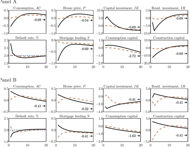
1.4.2.2 Capital technology shocks
Reaction of the model to capital technology shocks illustrates yet another dimension along which imperfect knowledge can improve the dynamics: co-movement of key observable variables. Panels A and B of figure 1.4 show responses due to a negative shock to capital technology’s persistent and transitory component, respectively. Consider the transitory shock first. It makes consumption sector’s capital more expensive in current period. In case of perfect knowledge, savers initially reduce consumption-capital investment and choose to allocate their wealth to consumption, construction capital, and housing purchases. Because of higher housing demand from savers, house price increases, default rate falls, and more expensive housing requires that borrowers get larger mortgages. Eventually, because of lower stock of consumption sector capital, output in consumption sector declines, together with aggregate consumption, house price, and capital investment in both sectors. Of course, consumption-sector capital is affected by this shock the most in the long run. Note that initially, the response is such that aggregate consumption, house price, and residential investment increase while capital investment declines.
The picture is the opposite for the persistent shock. The cost of consumption capital does not only increase in current period but keeps growing at a higher rate in subse-quent periods. In case of perfect knowledge, it means that investors not only pay more for consumption-sector capital; they expect it to be worth even more next period. In
ef-Panel A -0.69 Consumption,AC −1.0 −0.5 0.0 0.5 -0.54 House price,P −1.0 −0.5 0.0 0.5 -0.69 Capital investment,IK −5.0 0.0 5.0 10.0 -0.69 Resid. investment,IH −10.0 −5.0 0.0 5.0 Default rate, % 1.9 2.0 2.1 2.2 0 10 20 -0.69 Mortgage lendingS −1.0 −0.5 0.0 0 10 20 -2.72 Consumption capital −2.0 −1.0 0.0 1.0 0 10 20 -0.69 Construction capital −20.0 −10.0 0.0 10.0 0 10 20 -0.69 -0.69 -2.72 -0.69 -0.54 -0.69 -0.69 Panel B -0.41 Consumption,AC −0.5 0.0 0.5 -0.32 House price,P −0.5 0.0 0.5 -0.41 Capital investment,IK −4.0 −2.0 0.0 2.0 -0.41 Resid. investment,IH −5.0 0.0 5.0 Default rate, % 1.9 2.0 2.1 0 10 20 -0.41 Mortgage lendingS −0.5 0.0 0.5 0 10 20 -1.63 Consumption capital −2.0 −1.0 0.0 1.0 0 10 20 -0.41 Construction capital −5.0 0.0 5.0 0 10 20 -0.41 -0.41 -1.63 -0.41 -0.32 -0.41 -0.41
Figure 1.4: Impulse-responses. Panel A: persistent capital technology shock,vk. Panel B:
transitory capital technology shock, uk. Percentage deviations of non-detrended variables
from the balanced growth path due to one-standard-deviation negative shock. Solid lines represent the case of certainty; dashed lines represent uncertainty. For default rate, the values are absolute, compared with their steady-state values (dotted lines). Numbers near the arrows show where the deviations will stabilize after 400 quarters.
fect, the return on one unit of consumption good spent on consumption-sector capital rises, and savers increase investment into consumption sector at the cost of consumption, housing purchases, and construction-sector capital. The initial response is that aggregate consumption, house price, and residential investment decline while non-residential invest-ment rises. Eventually, all four observable variables stabilize below the pre-shock balanced growth path.
Imperfect knowledge improves the co-movement of capital investment with other vari-ables due to capital technology shocks. This is especially evident for persistent shock,