Correlated Compressive Sensing for Networked Data
Tianlin Shi Da Tang Liwen Xu Thomas Moscibroda
The Institute for Theoretical Computer Science (ITCS) Institute for Interdisciplinary Information Sciences
Tsinghua University, Beijing
Abstract
We consider the problem of recovering sparse correlated data on networks. To improve accu-racy and reduce costs, it is strongly desirable to take the potentially useful side-information of network structure into consideration. In this pa-per we present a novel correlated compressive sensing method called CorrCS for networked data. By naturally extending Bayesian compres-sive sensing, we extract correlations from net-work topology and encode them into a graphical model as prior. Then we derive posterior infer-ence algorithms for the recovery of jointly sparse and correlated networked data. First, we design algorithms to recover the data based on pairwise correlations between neighboring nodes in the network. Next, we generalize this model through a diffusion process to capture higher-order cor-relations. Both real-valued and binary data are considered. Our models are extensively tested on several real datasets from social and sensor networks and are shown to outperform baseline compressive sensing models in terms of recovery performance.
1
INTRODUCTION
Networked data, from domains such as social network of friends, hyper-linked networks of webpages and dis-tributed network of sensors, are becoming increasingly per-vasive and important in modern signal processing and ma-chine learning. Recent research has demonstrated com-pelling approaches to extract useful information from these networked data, including latent structure of social links (Kemp et al., 2004), community detection (Fortunato, 2010), etc. However, with the massive amount of data gen-erated at an exploding rate, conventional ways of collect-ing networked data are becollect-ing challenged, particularly when measurements are expensive and/or data are redundant.
Figure 1: A graphical illustration of Compressive Sensing (CS)and Correlated Compressive Sensing(CorrCS)on networked data. InCS, each sparse signalxi is recovered independently asyi; inCorrCS, they are recovered jointly with the network structure.
A significant finding of a large class of high-dimensional data over the last two decades is their inherent spar-sity (Cand`es and Wakin, 2008). As a robust tool to leverage the sparsity, Compressive Sensing (CS) (Donoho, 2006) has been developed to collect high-dimensional sparse data from their low-dimensional projections. With sufficiently sparse signals, compressive sensing is guaranteed to re-cover the original signal from fewer samples required by Shannon-Nyquist limit (Cand`es, 2006). Compressive sens-ing has therefore been sucessfully applied to attack vari-ous problems of data collection in a wide range of fields, such as medical imaging (Lustig et al., 2008), low-level vi-sion (Yang et al., 2008), etc.
Successful attempts have been made to apply compressive sensing to collect and analyze sparse networked data. For example, in studying large-scale sensor networks, the pi-oneering work by Luo et al. (2009) shows a successful scheme to efficiently gather spatially sparse sensor read-ings. For social networks, Compressive Network
Anal-ysis (Jiang et al., 2011) proposes a novel framework for clique detection. These approaches typically require find-ing a proper basis over the network topology so that data could be sparsely represented.
In many cases, however, it is unclear how the network topology could imply the sparse structure of the data, and therefore difficult to identify the sparse basis. Take the social network for example. It has been known that so-cial influence and correlation exist at a large statistical level (Backstrom et al., 2006), but it turns out hard to di-rectly model due to unobserved latent factors (Anagnos-topoulos et al., 2008). An interesting question would be, under uncertainty about correlation of sparse data across the network, is it possible to seriously incorporate the net-work structure into compressive sensing and hopefully to improve recover performance?
In this paper, we present Correlated Compressive Sensing (CorrCS) to solve this problem. In particular, the setting in Figure 1 is considered. Each nodeiis equipped with a sensor, and we aim to recover the original high-dimensional data xi from its low-dimensional measurements yi. In-stead of independently recover sparse signals,CorrCS in-corporates side-information of the network structure and build correlation into signal modeling jointly with the in-herent sparsity. By adopting a probabilistic approach, we show that it is possible to exploit the flexibility of graphical models to improve compressive sensing. Our approach is extensively tested on several real datasets, including prod-uct review data from social trust networks, social polling data and Air Quality Index from distributed sensors. The results show thatCorrCSoutperformsCSin terms of re-cover performance and demonstrates the usefulness of cor-relation in sensing networked data.
2
PRELIMINARY
In a typical sensing problem, the data of interest is regarded as a signal, which is a vector x in a high-dimensional spaceRr. A measurement ofxis a low-dimensional vec-tory∈Rm(m≤r)from which the information ofxcan be extracted. From a Bayesian point of view, this corre-sponds to inferringp(x|y) ∝ p(y|x)p(x). The likeli-hood termp(y|x)describes a sensing model, which is the noisy measurement process, and the termp(x)corresponds to a signal model, which represents the prior knowledge.
2.1 THE SENSING MODEL
A large body of sensing methods focus on the linear system
y=Vx (1)
with the goal to recover xfrom y accurately. However, sincerm, the inversion problem is highly ill-posed due to the undetermined solutions. One way to deal with the
uncertainty is to adopt a Gaussian generative model fory as follows,
y|x∼ N(Vx, β), (2) whereβ is the variance controlling the precision of mea-surement.
2.2 THE SIGNAL MODEL
Many natural signalsx∈ Rrcan be sparsely represented under some basisΦ= [φ1,φ2, ...,φK]as
x=Φz (3)
wherez is the sparse coefficients such that||z||0 =S
K. Compressive sensing (Donoho, 2006; Cand`es and Wakin, 2008) shows that if the signal x is sufficiently sparse, one can recover it effectively through minimizing the number of non-zero components inz:
min ||z||0
s.t. y=Mz (4)
where M = VΦ. In practice, it is often hard to solve the non-convex objective in (4) exactly, and a`1relaxation is usually adopted, which corresponds to the basis pursuit (BP) algorithm (Chen et al., 1998). Cand`es et al. (2006) have proved that, under certain isometry properties, one can recover xperfectly fromm = Ω(Slogr)observationsy through BP.
To allow extra flexibility that we would exploit later, the framework of CS could be reformulated approximately as a Bayesian inference problem (Ji et al., 2008), and its goal is to design a signal modelp(z;Γ)with some parameterΓ
so thatzis controlled to be sufficiently sparse. Below we describe two common sparse signal models in social and sensor networks.
`1 prior for real-valued z. Using sparsity-favoring Laplace priors on the coefficients (Babacan et al., 2010), one could use the following signal model:
p(z;λ) =λ K/2 2K exp −√λ||z||1 (5)
In practice, it is often inconvenient that the Laplace prior is not conjugate to the Gaussian signal model. However, one can show that (5) is equivalent to a hierarchical conju-gate model parametrized byΓ= ({γk}Kk=1, λ)(Seeger and Nickisch, 2008). p(z;Γ) = K Y k=1 N(zk; 0, γk) p(Γ) =Gamma(γk; 1, λ 2) (6)
The inference ofzfor (6) can be efficient via the EM algo-rithm (Dempster et al., 1977).
Beta process for binary z. An efficient way to charac-terize the sparsity of binary-valued coefficients is the Beta process (Paisley and Carin, 2009). In practice, a finite trun-cation of the process is used and leads to the following hi-erarchical conjugate model:
p(z;Γ) = K Y k=1 Bernoulli(zk;πk) (7) p(Γ) = K Y k=1 Beta(πk; a K, b(1− 1 K))
where Γ = ({πk}Kk=1, a, b)and a, b are hyper-prior af-fecting sparsity. The exact posterior inference of (7) is in-tractable, but can be approximated through MCMC (Mo-hamed et al., 2011) or mean-field variational infer-ence (Paisley and Carin, 2009).
3
CORRELATED COMPRESSIVE
SENSING
Now, consider the problem of collecting data distributed on a network of nnodes. When the network structure is known, it can be described by a graphG(V, E), where the edges have weight
Eij =
wij, nodeiandjare adjacent
0, otherwise , (8)
wherewij encodes the side-information about the correla-tion between the nodeiandj. In practice, such weight can either be collected directly from network or be computed through some metrics such as Pearson correlation and some function of geographic distance. When this weight is not exactly available, it is convenient to set wij = 1for all edges uniformly. Let (Z,X,Y) = {zi,xi,yi}n
i=1, the Bayesian formulation of sensing is generalized as the fol-lowing principle p(Z|Y)∝p(Z) N Y i=1 N(Mizi, β). (9)
Instead of applying compressive sensing independently to each node (i.e. p(Z) = Q
ip(z
i)), Correlated Compres-sive Sensing (CorrCS) fuses the network structureGinto recovery as side-information. To fulfill this goal, a joint distributionp(Z)is explored in this section to capture the notion of joint sparsity and correlation.
3.1 PAIRWISE CORRELATION
The simplest form of correlation among networked data is pairwise according to the edge connecting neighbor-ing nodes. Inspired by graphical models, we con-sider a range of pairwise Correlated Compressive Sensing
(CorrCS-Pair) that can be formulated as the Gibbs dis-tribution p(Z|Γ)∝exp−X i Si−c X (i,j)∈E Cij(zi,zj). (10)
whereSiis the sparsity of individual nodezicontrolled by hyper-parameterΓandCij models the pairwise correlation between two neighboring signal coefficients zi, zj. The parameterccontrols prior on the strength of correlation. Notice whenc= 0, equation (10) reduces to independently applying BCS to each node. And the biggercis, more cor-relation between neighboring nodes is favored over spar-sity. On networked data with inherent correlation, we would expectedly improve the recovery performance with proper choice of positivec. However, ifc→ ∞, the model would totally neglect sparsity, and therefore be undesirable. This variation of the recovery performance happens in ac-tual experiments, as will be discussed later.
Below we consider two specific forms ofCorrCSfor real-valued and binary networked data. We discuss their infer-ence algorithm in section 3.3.
Laplace-GRF Model. Assume Z = Rk×n. Often we have the prior knowledge that neighboring sparse coeffi-cient zi,zj are close. This intuition leads to combining Laplace prior and Gaussian Random Field (GRF). Let
Si=||zi||1
Cij =w
ij||zi−zj||2 . The distributionp(Z; Γ)is jointly Gaussian.
Beta-Ising Model. AssumeZ = {0,1}k×n. This case is appealing for potential social network applications. For example, zij could be a latent feature indicating whether userilikes the productj. The Beta process (7) enforces the sparsity of binary coefficients. And based on similar idea of closeness, the Ising model shows a way to incorporate pairwise correlation into the model:
Cij = K X k=1 wij(2zik−1)(2zjk−1). (11) 3.2 DIFFUSION PROCESS
We show that the pairwise correlation for real-valued sig-nals can be generalized through a Diffusion Process (DP) on the graphG. The Correlated Compressive Sensing with Diffusion Process (CorrCS-DP) characterizes the covari-ant structure of the latent signals with a generative model, whose zeroth-order approximation is compressive sensing, and first-order approximation is pairwiseCorrCS. Diffusion Process. For any graphG(V, E), a value func-tion f : V → Rcan be defined. Diffusion Process (DP)
is a natural class of stochastic processes on graphs that yields covariance structure of the functionf (Kondor and Lafferty, 2002). First, we extend our value function as a function of time t: define f[t] be the snapshot vector of
[f(v1), f(v2), ..., f(vn)]at time t. Next, a diffusion gen-eratorH is defined as a Laplacian matrix of graphGas:
Hij= wij fori6=jandj∈ A(i) −P i0wii0 for i = j 0 otherwise. (12)
ThenH is applied to the value function in the following way
∂f[t]
∂t =αHf[t]. (13)
Solving (13), we obtain
f[t] =Kf[0], (14) whereK= exp(αtH)is theDiffusion Kernel. Notice that heat kernel is always invertible, which means givenf[t]at any timetit is easy to computef[0] = exp(−αtH)f[t]. Notice that whent= 0,K =I; whentis small, we have the first-order approximationK=I−αtH.
Correlation via Diffusion.InCorrCS, we can definefk:
V → Rfor each dimension of the features asfki = z i k, so the snapshot fk is a vector. By studying the statistical characteristics offk, k= 1,2, ..., K, we can then build a correlated sparse signal modelp(Z), which is the core of CorrCS-DP.
Imagine thatfkis generated through the following process: Initially fk[0] is sparse. This means each entry fi
k[0]is distributed i.i.d as
fki[0]∼ N0, γki, ∀vi∈V (15) Hyper-parameters γi
k control the sparsity of each entry. They are both drawn from hyper-priors according to equa-tion (6).
A diffusion process is then run on the graphG(V, E)and stops at some time t producingfk[t] = Kfk[0]. Using the diffusion-based generative model, the inference prob-lem (9) for real-valued signals becomes
p(Z|Y;Γ)∝ Pr(Γ) exp−1 2 X k (fk)>(K−1)>DkK −1 fk −1 2β X i (yi−Mixi) > (yi−Mixi) (16)
whereDk =diag(γk)−1. Notice that in this formulation, we no longer need constantcto control the extent of corre-lation, since it is directly induced by the prior uncertainty
γki. A few observations can be made about the connec-tion ofCorrCS-DPto other compressive sensing methods summarized as follows.
Proposition 3.1. Using zeroth-order approximationK :=
I, where Iis the identity matrix, CorrCS-DPsubsumes BCS.
Proof. Straightforward. By replacingK :=Iin (16), the posteriorp(X|Y)is exactly the same as BCS.
Proposition 3.2. Using first-order approximationK :=
I−αtH,CorrCS-DPreduces toLaplace-GRFmodel. Proof. This claim is induced by the general property of Laplacian H that fk>Hf = P
ijwij(fki−f j
k)2. Using the first order approximation, we have
−logp(Z|Y;Γ)= 1 2 X ik (f k i γk i )2−αtX k (fk)>DkHfk +Const (17) Letdk
i = 1/(γki)2. NoticeH is a Laplacian matrix,
−(fk)>DH kfk= X ij wij dki(fik)2+dkj(fjk)2 −(dki +dkj)fikfjk =X ij wij( di+dj 2 )(f k i −f k j) 2 −αt 2 X i (Hdk)i Let S= 1 2 X ik (fik)2((I− αt 2 )d k) i and Cij =wij( di+dj 2 )(f k i −fjk)2, then p(X|Y;Γ) ∝ exp(−S − P ijCij) shows that Corr-DPreduces to a pairwise correlation model.
3.3 INFERENCE ALGORITHM
The exact inference ofCorrCSis largely intractable due to two reasons. First, the signal model and the sensing model is not in same conjugate family. Second, even ifp(X;Γ)is jointly Gaussian, in real applications either the number of nodes or the dimension of features is big.
Instead, we resort to approximation methods and de-velop the posterior inference based on Variational Bayes EM (Bernardo et al., 2003). In particular, we use the mean-field approximation p(X|Y;Γ) = Q
ikq(zik;Γ) and perform the following two-step scheme. In the E-step, we propagate information across nodes to spread cor-relation, which can be related to a message-passing pro-cess (Donoho et al., 2009); in the M-step, we updateΓto enforce sparsity. The details are outlined in Algorithm 1.
Algorithm 1Correlated Compressive Sensing
1: Input: NetworkG(V, E),Y = [y1,y2, ...,yn], basis
Φ, measurement matricesVianditer. 2: fori= 1→ndo
3: computeMi=ViΦfor alli= 1,2, ..., n. 4: initializezi= (Mi)>yi. 5: end for 6: forj= 1→iterdo 7: fori= 1→ndo 8: fork= 1→kdo 9: Update factorqi k(z i k)using equation (19), (20), (21). 10: end for 11: end for 12: fori= 1→ndo
13: For binary case, use equation (22) to updateπi; for real-valued case, use equation (24) to update γi.
14: end for 15: end for
E-Step: Spread Correlation.
In the pairwise case, the update algorithm in general is
qi(zki)∝exp Eq(zi ¬k)[ 1 2β||y i−Mizi||2+S i] +c P j∈A(i) Eqj(zj)[Cij+Cji] . (18)
wherez¬ikdenotes all variables inziexceptzki. Intuitively, the first expectation in (18) propagates information across dimensions of zi, while the second expectation in (18) spreads correlation among different nodes on the graph via the edges in between. Notice that for directed networks
wij 6= wji, the information propgates forward and back-ward the edge in the same way, due to the symmetry of
Cij+Cij.
Specifically, forBeta-Isingmodel,
q(zi k= 1) ∝πkiexp −1 2β(M i k)>(Mki) −2(Mki)>(yi−M¬ikE[zi¬k]) +c P j∈A(i) (wij+wji)(2zki −1) q(zik= 0) ∝1−πki. (19)
Similarly for Laplace-GRF model, the mean-field up-date for each factor isqi
k(zki) =N(µik, σki), where σik= (β(Mki)>Mki+ 1/γki)−1 µi k=σki · β(Mi k)>(yi−M¬ikµi¬k) +c P j∈A(i) (wij+wji)µjk . (20)
whereµi¬k denotes all entries inµiexceptµik. For the ex-tention of Laplace-GRFmodel, CorrCS-DPcontains long-range interaction among the node, so all other nodes contribute to the distribution of the current node being up-dated. As in Laplace-GRF, we still have qi
k(z i k) = N(µi k, σ i k), but instead σi k= β(Mi k)>M i k+U k ii −1 µi k=σ i k· β(Mi k) >(yi−Mi ¬kµ i ¬k) + P j∈V (Uk ¬i+ (Uk)>¬i)>u j k . (21) whereUk =K−TDkK−1anduk = [µ1k, µ 2 k, ..., µ n k]. Iteratively updating the factors according to equation (20), (19) and (21) guarantees convergence (Wainwright and Jor-dan, 2008).
M-Step: Update hyper-parameters. With the expec-tation of current belief about the signal to recover, we can further update the hyper-parametersΓto enforce spar-sity based on EM algorithm (Dempster et al., 1977). For Beta-Ising, we update the parameters of the Bernoulli priorπi
kas follows
πik∼ a/K+E[zk]−1
a/K+b(1−1/K)−1. (22)
ForLaplace-GRF, we update the global parameters
γki =− 1 2λ2 + r 1 4λ2+ (σi k+ (µik)2) λ . (23)
The update of γki in CorrCS-DP is similar to Laplace-GRF. Specifcally, letQk be a diagonal matrix at timetsuch thatQkii=σik, computeQek =K−1QkK−>, which can be regarded as the uncertainty aboutfk[0]. Then we modify (24) as γki =− 1 2λ2+ s 1 4λ2 + e Qk ii λ . (24)
Combining E-step and M-step, we can jointly optimizeΓ
and inferZ, which eventually recovers the networked data on the graphG.
4
EXPERIMENT
We evaluate Correlated Compressive Sensing (CorrCS) empirically on real datasets from social and sensor net-works with pairwise or Diffusion-like correlation.
4.1 SOCIAL NETWORK DATA WITH PAIRWISE CORRELATION
Using compressive sensing with pairwise correlation, we test the two recovery models Laplace-GRF and Beta-Isingon two datasets: product review on Epin-ion1and consumer polling data in Michigan.
4.1.1 Performance on different datasets
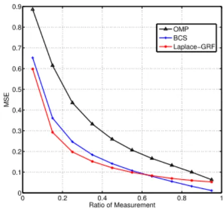
Michigan Polling Data. The social polling data is col-lected from a survey of consumers in Michigan with 500 monthly telephone calls from January, 1978 to December 2012. The data is real-valued aggregation of four hundred economic indices. It has been known that pairwise corre-lation exists in these indices. Using half of the dataset as past history, this pairwise correlation is computed through Pearson correlation and taken as the weightwij. Therefore, we establish a graph of features representing their inherent correlation. Furthermore, the data is continuous real values and to sparsify it, we use online sparse matrix factoriza-tion (Mairal et al., 2010) to find a set of sparse basis. We test Laplace-GRFmodel on the Michigan polling data with a = 1, b = 0.1andc = 1. As measurements, we randomly select a fraction of the polling data for each feature. We refer to the dimension of the selected data ver-sus the dimension of the original data as measurement ra-tio. The performance is evaluated via Mean Squared Error (MSE) of the recover signal with respect to the original one. The MSE is normalized by the 2-norm of the original sig-nal. For independent compressive sensing, we include two popular choices – Bayesian Compressive Sensing (Ji et al., 2008)(BCS) and Orthogonal Matching Pursuit (Tropp and Gilbert, 2007)(OMP) – as baseline algorithms. Notice that some baseline implementations of compressive sensing, such as Basis Pursuit (Chen et al., 1998)(BP), are too slow and impractical for networked data.
The result is reported in Figure 2. As we can see, Laplace-GRF outperforms BCS and OMP largely for small measurement ratios (less than 0.6). When the mea-surement ratio is large (exceed 0.6), Laplace-GRFwill have a performance similar to BCS, and it still outperform OMP to a big extent. Correlation is less useful for large measurement ratios, mainly because the numbers of obser-vations are already sufficient for sparse recovery. However, since in practice, people usually use a measure ratio in the rang[0.2,0.5], and rarely measure more than60% of the data for recovering. Hence, this will not have strong influ-ence onLaplace-GRF’s practical use.
To measure the superiority of Laplace-GRF for small measurement ratio, we could compare the minimum mea-surement ratio that is needed to achieve a fixed accuracy level (i.e. MSE level) for different models. Like in this
1 Available attrustlet.org. 0 0.2 0.4 0.6 0.8 1 0 0.1 0.2 0.3 0.4 0.5 0.6 0.7 0.8 0.9 Ratio of Measurement MSE OMP BCS Laplace−GRF
Figure 2: Performance of Laplace-GRFmodel versus the BCS model and OMP on the polling data.
dataset, we compare the minimum measurement ratio for different models to achieve a MSE not more than 0.2: our Laplace-GRFneeds a measurement ratio of 0.23, BCS needs 0.32, while the most common baseline algorithm OMP needs 0.56. We could see that, to achieve this same recovery effect,Laplace-GRFneeds21%less measure-ments than BCS, and 59%less measurements than OMP. This result may imply that Laplace-GRFmodel could have valuable practical use since we could use a small num-ber of measurements to recover a polling result, which is very close to the original ones. And by considering the in-herent correlation between these indices, we could reduce the number of measurements by a ratio of21%to recover a result with MSE 0.2 on this data, which means we could save a great deal of costs for this poll.
Epinion Data. The Epinion data is derived from the social product review network Epinions with 17,022 customers and 139,738 products. The graphGis built from the trust-list of all users: wij = 1if and only if useritrusts userj, and therefore it is directed. To reduce the dimensionality of features, we select a subset of the most 100 popular prod-ucts. Thenzij represents whether customeriliked product
j. The dataZis inherently sparse with only 5 to 10 nonzero per column, because the fraction of products rated by each customer is small. As measurements, each column zi is projected to a low-dimensional space.
We test Beta-Ising model on the Epinion dataset against Bayesian Compressive Sensing (BCS) with beta prior. We choose λ = 1, c = 0.3. For the binary Epin-ion data, MSE is not a good choice because the data is zero almost everywhere. Instead, we regard the recovery as pre-dicting label zij and use F1 score from classifier evalua-tions, which is the harmonic mean of precision (ratio of number of correct 1’s we recover over the total number of 1’s in our recovery result) and recall (ratio of number of correct 1’s we recover over the total number of 1’s in the ground truth).
0 0.2 0.4 0.6 0.8 1 0 0.1 0.2 0.3 0.4 0.5 0.6 0.7 0.8 0.9 1 Ratio of Measurement F1 Score BCS Beta−Ising
Figure 3: Performance ofBeta-Isingmodel versus the Bayesian-Compressive Sensing on the Epinion data.
Figure 3 shows the result under F1 score. It can be seen that with correlation, the performance of BCS can be improved with a varying number of measurement ratios.
In our experiment, Beta-Ising model takes approximately the same amount of time for one iteration as BCS does, which indicates that it is a feasible and practical method for recovering binary networked data.
4.1.2 Sensitivity evaluation
Impact of parameters. In these two datasets, all parame-ters we could set are the parameter of the hierarchical con-jugate priora, b, λand weightc. As has been discussed in BCS (Ji et al., 2008), our models are not sensitive the pa-rametersa, b, λ. So in this paper, we focus on the impact of the weight parametercon the performance of theCorrCS models.
The choice ofcis the key toCorrCS, which can be viewed as a regularization parameter controlling the tradeoff with sparsity. To evaluate the impact of the c on the perfor-mance, we test the variation of the behavior of theCorrCS model on different scenario. For example, consider the Beta-Ising model on the Epinion data, we compare the variation of the recovery F1 score corresponding to the change of c when some reasonable measurement ra-tios are selected (15%,25%and35%). Figure 4 shows that among all these 3 measurement ratios, the performance of this model will be improved when c starts to grow from 0, and will be demoted whencpass some specific values. This result accords with our discussion aboutcin Section 3.1. This kind of variation of the performance according to
c’s variation is reasonable since different values ofcimply different extents that we care about the inherent correlation between nodes in the network structure. This experiment show us that the performance will have the same trends of
0 0.2 0.4 0.6 0.8 1 1.2 1.4 1.6 1.8 2 0.4 0.45 0.5 0.55 0.6 0.65 0.7 0.75 0.8 0.85 0.9 Weight Parameter (C) F1 Score mratio = 15% mratio = 25% mratio = 35%
Figure 4: Relationship between the performance of the Beta-Ising model and the parametercon different measure ratios.
variation on different measurement ratios whencis chang-ing.
It is worth noting that among the 3 reasonable measurement ratios, the bestc’s that will induce an optimal performance are very close. As shown in Figure 4, the model will pos-sess an optimal performance whencis some value among 0.3. Ifc = 0.3, then the model will always have a nearly optimal recovery result as long as the measurement ratio is in a reasonable range. Therefore, in this model, we could choose an optimal choice of cthat works well on all rea-sonable cases.
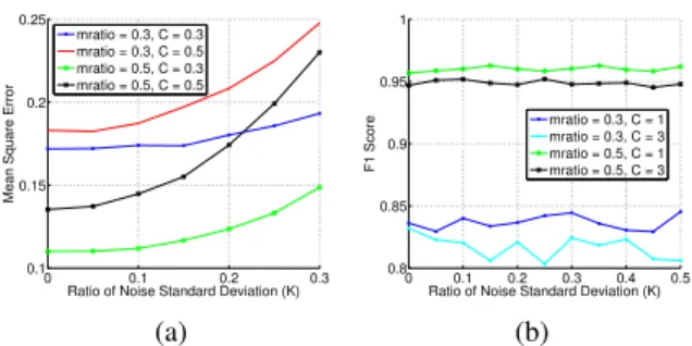
Impact of noise on the measured data. To test the ro-bustness of these two models, we test the performance of our model on the two datasets when noises are added. More precisely, we add a Gaussian noise at each dimension of the observationy, where the standard deviation of this noise at each dimension isκtimes the original value of this dimen-sion, whereκis Signal-to-Noise Ratio. We test the perfor-mance of the two models asκincreases from0to0.5on different scenarios (i.e. different measure ratios and weight parameters). As can be seen in Figure 5, this two models possess strong robustness on the two datasets since even if
κgoes to 0.5 the recovery result will not vary too much. The Beta-Ising model on the Epinion dataset has a slightly better robustness than that of theLaplace-GRF model on the polling dataset since it deals with binary vari-ables, whose robust recovery turns out to be easier.
4.2 POLLUTION DATA FROIM SENSOR
NETWORK
The Beijing pollution data includes a network of 22 mon-itoring stations collecting data in the same time window
0 0.1 0.2 0.3 0.1
0.15 0.2 0.25
Ratio of Noise Standard Deviation (K)
Mean Square Error
mratio = 0.3, C = 0.3 mratio = 0.3, C = 0.5 mratio = 0.5, C = 0.3 mratio = 0.5, C = 0.5 (a) 0 0.1 0.2 0.3 0.4 0.5 0.8 0.85 0.9 0.95 1
Ratio of Noise Standard Deviation (K)
F1 Score mratio = 0.3, C = 1 mratio = 0.3, C = 3 mratio = 0.5, C = 1 mratio = 0.5, C = 3 (b)
Figure 5: Robustness ofCorrCSon the 2 datasets when some noise is added to the measure.(a). Robustness of the Laplace-GRF model on the Polling dataset. (b). Robust-ness of the Beta-Ising model on the Epinion dataset
0 0.1 0.2 0.3 0.4 0.5 0.6 0.7 0.8 0.9 1 0 0.1 0.2 0.3 0.4 0.5 0.6 0.7 0.8 0.9 1 Ratio of Measurement
Mean Square Error
Accuracy of CorrCS−DP on Air Quality Dataset
CorrCS−DP BCS OMP
Figure 6: Performance of CorrCS-DP on Air Quality Dataset. Recovery accuracy of CorrCS-DP compared with BCS and OMP.
from Feb. 8th 2013 to Dec. 17 2013. The Air Quality Indexes (AQI) PM2.5 is recorded at an interval of 1 hour. The geography information of the sensors are available as GPS coordinates(gi, li), which we use to compute the edge weight of the sensor network through their euclidean dis-tanceeij= exp(−θ
p
(gi−gj)2+ (li−lj)2).
The time sequence data is divided into 22 chunks, with 2 weeks of pollution data each chunk. The data is then split into two parts. Then we use 11 chunks to train a set of sparse basis using online sparse matrix factoriza-tion (Mairal et al., 2010), and also as cross-validafactoriza-tion to find the best choice of diffusion timet = 0.1andc = 5. The rest 11 chunks are used to testCorrCSand its coun-terparts. To simulate a real setting of measurement, we ran-domly select a portion of the samples as measurement and try to recover the rest. To test recovery accuracy in vari-ous situations, we change the ratio of measurement from 0 to 1 and compute the mean square error of the recovered signals.
Figure 6 and 7 shows the recovery accuracy and conver-gence rate of CorrCS-DPon the pollution dataset with comparison to the compressive sensing counterparts. The
0 2 4 6 8 10 12 14 16 18 20 0 0.05 0.1 0.15 0.2 0.25 0.3 0.35 0.4 Ratio of Measurement
Mean Square Error
Convergence of CorrCS−DP on Air Quality Dataset
0.1 0.25 0.4 0.55 0.7
mratio
Number of Iterations
Figure 7: Convergence of recovery accuracy with number of iterations.
Objective MSE CorrCS-DP OMP BCS 0.1 0.30 0.60 0.54 0.15 0.18 0.41 0.43 0.2 0.13 0.29 0.35 Table 1: Minimum measurement ratio to reach some partic-ular values of MSE on the AQI dataset on different models
results are averaged over 10 independent runs. From Figure 6 we can see thatCorrCSlargely improves the recovery accuracy for various ratio of measurement, due to exploit-ing the correlation among different nodes. To measure the improvement ofCorrCS-DPcomparing to the other two models precisely, we could again compare the necessary minimum measurement ratio to reach some particular val-ues of MSE on this data set on different models. As shown in Table 1, to reach the same MSE, CorrCS-DPcould measure at least40%less data than the other two models. Furthermore, as shown in Figure 7,CorrCSconverges in about 3-4 steps. The convergence is faster than both OMP and BCS, and therefore demonstrates CorrCS-DP to be an efficacious and pragmatic correlated-recovery model.
5
RELATED WORK
Last two decades have witnessed significant advances in the theory and application of sensing sparse signals. Com-pressive sensing exploited the fact that natural signals are sparse and compressive under proper basis and de-signed sampling algorithms beyond the Nyquist-Shannon limit (Cand`es and Wakin, 2008). The theory of compres-sive sensing was developed by Cand`es et al. (2006) to explain this novel recovery performance. This theory was further improved by Cand`es and Tao (2006) to account for noisy measurements. The underlying property empower-ing sparse recovery is Restricted Isometry Property (RIP) of measurement matrices (Cand`es, 2008). On the algorith-mic side, the first attempts to solve compressive sensing problems rely on `1 minimization under linear program-ming (Chen et al., 1998; Cand`es and Tao, 2005). Instead of optimizing with a large number of constraints,
Orthog-onal Matching Pursuit (Tropp and Gilbert, 2007) used a greedy heuristic to find solutions close to`0optimum. To facilitate large-scale applications, Donoho et al. (2009) bor-rowed ideas from graphical models and derived a message passing algorithm for compressive sensing.
The Bayesian formulation of compressive sensing (BCS) is first proposed by Ji et al. (2008), which used a tractable conjugate Gamma prior on signal precision to enforce spar-sity. It was shown that Bayesian compressive sensing al-lows uncertainty estimate and adaptive sampling. Based on BCS, Ji et al. (2009) developed a multi-tasking com-pressive sensing algorithm that allows simultaneously data collection from multiple sensors. Babacan et al. (2010) showed that stronger sparsity can be achieved for BCS with an conjugate prior on signal variance that is equivalent to the Laplace prior. As a counterpart of Laplace prior, beta prior is also commonly used (Paisley and Carin, 2009), with an additional latent variable controlling the support of signals. By comparing Laplace and Beta priors for sparse representation, Mohamed et al. (2011) concluded that Beta prior enforced stronger sparsity than the Laplace prior. Real data is typically not sparse and therefore one must take effort in finding the appropriate basis. With a data-drive approach, dictionary learning for sparse basis orig-inated from efforts in reproducing V1-like visual neu-rons through sparse coding (Olshausen and Field, 1997). Aharon et al. (2006) generalized the K-means clustering al-gorithm, and computed sparse decomposition by iteratively updating sparse coefficients and dictionary items. Mairal et al. (2009) proposed online dictionary learning methods, which leads to efficient computation of sparse coding. Compressed sensing has find great applications in sensor networks. It was first successfully applied to network mon-itoring for optical and all-IP networks (Coates et al., 2007). In terms of data gathering, Luo et al. (2009) constructed a sensor network with a sink collecting compressed mea-surements, which is equivalent to a random matrix projec-tion. Xu et al. (2013) considered more general compressed sparse functions for sparse representation of signals over graphs. Other than collecting data, compressive sensing was also used as a network analysis tool to identify social community on graphs (Jiang et al., 2011).
The topic of correlation in compressive sensing has been explored preliminarily in various ways. Shahrasbi et al. (2011) used belief propagation to handle time-correlated signals with compressive sensing. Arildsen and Larsen (2014) explores the correlation of signal and measurement noise. In terms of networked data, Feizi et al. (2010) con-siders a distributed setting and a joint recovery model. As far as we know, our work is the first to explicitly incorpo-rate graph structure as a hint of correlation.
Diffusion process has long been used as a general tool to capture correlation among data (Kondor and Lafferty,
2002). Ma et al. (2008) used diffusion process to model marketing candidate selection in social networks. The dif-fusion process may also be utilized to produce an represent-ing wavelet basis on graphs and manifolds (Bremer et al., 2006). Using diffusion wavelets, it is possible to sparsify signals on different graph topologies and allow compres-sive sensing (Haupt et al., 2008). However, our correlated compressive sensing does not rely on the strong assump-tion that data on the network should be sparse under some basis, but rather weakly correlated.
6
CONCLUSIONS AND FUTURE WORK
In this paper, we present Correlated Compressive Sensing (CorrCS) to leverage correlation among networked data and to empower better sparse recovery. Using a Bayesian approach,CorrCSallows flexible representation of prior knowledge about correlation via a graphical model. Two common types of correlation of networked data are consid-ered: pairwise and diffusion-based. We have shown the diffusion-based formulation subsumes the pairwise case via a low-order approximation. Through extensive empir-ical evaluation on real data on social and sensor networks, we have demonstrated the advantage of correlated com-pressive sensing over its counterparts.
As future work, we are interested in showing bounds in its recovery performance to better understand its properties. Also we are interested in developing nonparametric exten-sions of the current approach to allow adaptive inference of key parameters and the basis for sparse representation.
7
ACKNOWLEDGEMENT
This work was supported in part by the National Ba-sic Research Program of China Grant 2011CBA00300, 2011CBA00302, the National Natural Science Foundation of China Grant 61073174, 61033001, 61361136003, and the Hi-Tech research and Development Program of China Grant 2006AA10Z216.
References
Aharon, M., Elad, M., and Bruckstein, A. (2006). K-SVD: An algorithm for designing overcomplete dictionaries for sparse representation. Signal Processing, IEEE Transactions on, 54(11):4311–4322.
Anagnostopoulos, A., Kumar, R., and Mahdian, M. (2008). In-fluence and correlation in social networks. InSIGKDD, pages 7–15. ACM.
Arildsen, T. and Larsen, T. (2014). Compressed sensing with lin-ear correlation between signal and measurement noise. Signal Processing, 98:275–283.
Babacan, S. D., Molina, R., and Katsaggelos, A. K. (2010). Bayesian compressive sensing using laplace priors.Image Pro-cessing, IEEE Transactions on, 19(1):53–63.
Backstrom, L., Huttenlocher, D., Kleinberg, J., and Lan, X. (2006). Group formation in large social networks: member-ship, growth, and evolution. InSIGKDD, pages 44–54. ACM. Bernardo, J., Bayarri, M., Berger, J., Dawid, A., Heckerman, D., Smith, A., West, M., et al. (2003). The variational Bayesian EM algorithm for incomplete data: with application to scoring graphical model structures.Bayesian statistics, 7:453–464. Bremer, J. C., Coifman, R. R., Maggioni, M., and Szlam, A. D.
(2006). Diffusion wavelet packets.Applied and Computational Harmonic Analysis, 21(1):95–112.
Cand`es, E. J. (2006). Compressive sampling. InProceedings of the international congress of mathematicians, volume 3, pages 1433–1452. Madrid, Spain.
Cand`es, E. J. (2008). The restricted isometry property and its implications for compressed sensing.Comptes Rendus Mathe-matique, 346(9):589–592.
Cand`es, E. J., Romberg, J., and Tao, T. (2006). Robust uncer-tainty principles: Exact signal reconstruction from highly in-complete frequency information. Information Theory, IEEE Transactions on, 52(2):489–509.
Cand`es, E. J. and Tao, T. (2005). Decoding by linear pro-gramming. Information Theory, IEEE Transactions on, 51(12):4203–4215.
Cand`es, E. J. and Tao, T. (2006). Near-optimal signal recovery from random projections: Universal encoding strategies? In-formation Theory, IEEE Transactions on, 52(12):5406–5425. Cand`es, E. J. and Wakin, M. B. (2008). An introduction to
compressive sampling. Signal Processing Magazine, IEEE, 25(2):21–30.
Chen, S. S., Donoho, D. L., and Saunders, M. A. (1998). Atomic decomposition by basis pursuit. SIAM journal on scientific computing, 20(1):33–61.
Coates, M., Pointurier, Y., and Rabbat, M. (2007). Compressed network monitoring for IP and all-optical networks. In SIG-COMM, pages 241–252. ACM.
Dempster, A. P., Laird, N. M., Rubin, D. B., et al. (1977). Max-imum likelihood from incomplete data via the EM algorithm.
Journal of the Royal statistical Society, 39(1):1–38.
Donoho, D. L. (2006). Compressed sensing.Information Theory, IEEE Transactions on, 52(4):1289–1306.
Donoho, D. L., Maleki, A., and Montanari, A. (2009). Message-passing algorithms for compressed sensing. PNAS, 106(45):18914–18919.
Feizi, S., M´edard, M., and Effros, M. (2010). Compressive sens-ing over networks. In Communication, Control, and Com-puting (Allerton), 2010 48th Annual Allerton Conference on, pages 1129–1136. IEEE.
Fortunato, S. (2010). Community detection in graphs. Physics Reports.
Haupt, J., Bajwa, W. U., Rabbat, M., and Nowak, R. (2008). Com-pressed sensing for networked data. Signal Processing Maga-zine, IEEE, 25(2):92–101.
Ji, S., Dunson, D., and Carin, L. (2009). Multitask compressive sensing. Signal Processing, IEEE Transactions on, 57(1):92– 106.
Ji, S., Xue, Y., and Carin, L. (2008). Bayesian compressive sens-ing. Signal Processing, IEEE Transactions on, 56(6):2346– 2356.
Jiang, X., Yao, Y., Liu, H., and Guibas, L. (2011). Compressive network analysis.arXiv preprint arXiv:1104.4605.
Kemp, C., Griffiths, T. L., and Tenenbaum, J. B. (2004). Discov-ering latent classes in relational data.
Kondor, R. I. and Lafferty, J. (2002). Diffusion kernels on graphs and other discrete input spaces. In ICML, volume 2, pages 315–322.
Luo, C., Wu, F., Sun, J., and Chen, C. W. (2009). Compressive data gathering for large-scale wireless sensor networks. In Mo-biCom, pages 145–156. ACM.
Lustig, M., Donoho, D. L., Santos, J. M., and Pauly, J. M. (2008). Compressed sensing MRI.Signal Processing Magazine, IEEE, 25(2):72–82.
Ma, H., Yang, H., Lyu, M. R., and King, I. (2008). Mining social networks using heat diffusion processes for marketing candi-dates selection. InCIKM, pages 233–242. ACM.
Mairal, J., Bach, F., Ponce, J., and Sapiro, G. (2009). Online dictionary learning for sparse coding. In ICML, pages 689– 696. ACM.
Mairal, J., Bach, F., Ponce, J., and Sapiro, G. (2010). Online learning for matrix factorization and sparse coding. JMLR, 11:19–60.
Mohamed, S., Heller, K., and Ghahramani, Z. (2011). Bayesian and L1 approaches to sparse unsupervised learning. arXiv preprint arXiv:1106.1157.
Olshausen, B. A. and Field, D. J. (1997). Sparse coding with an overcomplete basis set: A strategy employed by V1? Vision research, 37(23):3311–3325.
Paisley, J. and Carin, L. (2009). Nonparametric factor analysis with beta process priors. InICML, pages 777–784. ACM. Seeger, M. W. and Nickisch, H. (2008). Compressed sensing
and Bayesian experimental design. InICML, pages 912–919. ACM.
Shahrasbi, B., Talari, A., and Rahnavard, N. (2011). TC-CSBP: Compressive sensing for time-correlated data based on belief propagation. InCISS, pages 1–6. IEEE.
Tropp, J. A. and Gilbert, A. C. (2007). Signal recovery from ran-dom measurements via orthogonal matching pursuit. Informa-tion Theory, IEEE TransacInforma-tions on, 53(12):4655–4666. Wainwright, M. J. and Jordan, M. I. (2008). Graphical models,
exponential families, and variational inference. Foundations and Trends in Machine Learning, 1(1-2):1–305.
Xu, L., Qi, X., Wang, Y., and Moscibroda, T. (2013). Efficient data gathering using compressed sparse functions. In INFO-COM, 2013 Proceedings IEEE, pages 310–314. IEEE. Yang, J., Wright, J., Huang, T., and Ma, Y. (2008). Image
super-resolution as sparse representation of raw image patches. In