Price-Induced Technological Change in Italian Agriculture:
An SGM Restricted Cost Function Approach (1951-91)
Roberto Esposti
Department of Economics
Polytechnic University of Marche (Ancona – Italy)
and
Pierpaolo Pierani
Department of Economics
University of Siena (Italy)
Paper prepared for presentation at the XI
thCongress of the EAAE
(European Association of Agricultural Economists),
‘T
Th
he
e
F
Fu
ut
tu
ur
re
e
o
of
f
R
Ru
ur
ra
al
l
E
Eu
ur
ro
op
pe
e
i
in
n
t
th
he
e
G
Gl
lo
ob
ba
al
l
A
Ag
gr
ri
i-
-F
Fo
oo
od
d
S
Sy
ys
st
te
em
m’, Copenhagen, Denmark
August 24-27, 2005
Copyright 2005 Roberto Esposti and Pierpaolo Pierani. All rights reserved.
Readers may make verbatim copies of this document for non-commercial
purposes by any means, provided that this copyright notice appears on all such
copies.
PRICE-INDUCED TECHNOLOGICAL CHANGE IN ITALIAN
AGRICULTURE:
A SGM RESTRICTED COST FUNCTION APPROACH (1951-91)
Roberto Esposti
#and Pierpaolo Pierani
AbstractThis paper aims at investigating the price-induced innovation hypothesis in Italian agriculture over the years 1951 to 1991. Price-inducement hypothesis is analysed and tested within the framework proposed by Peeters and Surry (2000). The major difference is the short-run specification of the dual technology. Distinguishing between variable and quasi-fixed inputs allows both a more realistic representation of how relative prices may affect innovation and input use over time and a detailed decomposition of the relevant biases in input use. Results provide evidence in favour of price-inducement innovation in Italian agriculture.
Keywords: Induced Innovation, Italian Agriculture, SGM Restricted Cost Function JEL Classification: Q16
Introduction
This paper is primarily concerned with the investigation of price-induced innovation on technological change in Italian agriculture. The role of both autonomous technological change and R&D expenditure in Italian agriculture after world war II has received a great deal of attention (Pierani and Rizzi, 1994; Esposti, 1999; Esposti and Pierani, 2000; 2003b; 2005). Despite that, there is not much empirical evidence on the price inducement hypothesis and the few econometric findings are not clear-cut, perhaps due to the fact that the mechanism of the inducement is taken into account differently across different approaches.
Recently, Peeters and Surry (2000) (hereafter P-S) have proposed a dual model, which explicitly consider the time lags involved in the innovation process. In that paper, the induced technological change is cast within a partial adjustment framework involving lagged input prices that directly enter an symmetric generalized McFadden (SGM) multi-output cost function. In this paper, we depart from them by introducing quasi-fixed inputs, hence moving to a temporary equilibrium setting. As consequence, now lagged prices affect only variable input use, given the short-run fixity of the given capacity, which represents a structural constraint on the agricultural technology.
Distinguishing between variable and quasi-fixed inputs allows for a more realistic representation of the inducement mechanism and permits a comprehensive decomposition of the changes of variable input proportions over time, too. In principle, the overall bias can be attributed to pure-substitution, autonomous and price-induced technological change, expansion and capacity utilization (Morrison, 1988).
The paper is organised as follows. The second section shortly reviews the price-inducement literature, paying attention to the empirical application to the agricultural sector and the improvements and developments proposed in recent works. The third section presents the short-run SGM cost function used to model Italian agriculture. The study focuses on the role of the lagged prices of
# Corresponding author:
Roberto Esposti
Department of Economics - Polytechnic University of Marche Piazza Martelli, 8 - 60121 Ancona - Italy
Tel. 071-220.71.19; Fax 071-220.71.02 [email protected]
www.dea.unian.it/esposti
The authors are listed alphabetically and authorship may be attributed as follows: sections 1, 3, 5 and 7 to Pierani; sections 2, 4 and 6 to Esposti. We wish to thank two anonymous referees for their useful suggestions on a previous version of the paper.
variable inputs and the measures of price-inducement; thus, the relevant elasticities and biases are detailed in the forth section. The fifth section shortly describes the data set and the estimation method, while the sixth section discusses the empirical results. The seventh section concludes and suggests some possible directions of future research on this topic.
The price-induced innovation in agriculture: an overview
Since Hayami and Ruttan (1970), the separation of the effect of relative price changes in pure-substitution and technical change inducement has been the major theoretical as well as empirical issue in attempting to test the inducement hypothesis as originally formulated by Hicks (1932). Within a dual representation of technology, Binswanger (1974) tested this hypothesis by a two-stages approach: firstly estimating the technical change biases, and then relating them to the respective relative price changes. In fact, the specification of the inducement mechanism as a two-stages process has become popular since the mid-sixties, alias the induced innovation hypothesis (Ahmad, 1966; Hayami and Ruttan, 1970, 1985; Thirtle, 1985). The induced innovation hypothesis states that changes in relative prices provide signals to the research community thus affecting the direction of research and innovative activities; these innovations then allow the producers to adopt new techniques where the factor proportion is, ceteris paribus, now biased against the scarce input.
The induced innovation hypothesis has also received some attention within the agricultural economics literature (Koppel, 1995; Sunding and Zilberman, 2001). A major reason is that it was formulated by Hayami and Ruttan just to explain patterns of agricultural development over different conditions in terms of resource scarcity. Another reason can be detected in the attempt to explain how a sequence of radical technological breakthroughs (mechanical, chemical, biological, biotechnological, etc.) determined remarkable changes in agricultural factor proportion in the last century, particularly in the capital/labour and in land/labour ratio. In this respect, this formulation of the induced innovation theory is particularly appealing as it highlights the role played by the complex institutional system (external to farms) traditionally delivering agricultural research and innovations within developed and developing countries (the so-called National Agricultural Research Systems, NARS).
Since seventies, several empirical papers has attempted to test this induced innovation hypothesis in the agricultural context with mixed results, usually within the neoclassical production framework, but also contesting the Hayami and Ruttan conclusions on an historical base (Olmstead and Rhode, 1994). In particular, in the last decade a lot of contributions have shed new light on this subject. With respect to the previous tradition, the general purpose of this recent research effort is to put more emphasis on the time dimension the inducement process. It is, by definition, a medium and long-term process implying a sequence of events, involving relative prices, R&D investment and change in factors proportion in a specific causal chain. Therefore, the temporal consistency of the inducement representation within the usual neoclassic production framework has become the critical empirical issue.
In this respect, we can distinguish the recent empirical literature on the subject in two directions. On the one hand, several applications try to arrange and implement consistent methodological approaches to specifically focus on the time-consistency issue, but still respecting the Hayami and Ruttan original intuition and framework. On the other hand, however, other empirical works focused on a different theoretical representation of the inducement process (we can call it price-induced or
price-conditional technology), where lagged prices directly enter the primal or dual representation of technology and the consequent firms’ behavioural equations.
The former stream of research generally aims at testing the induced innovation hypothesis by empirically implementing somehow the two-stages sequence implied by the Hayami and Ruttan model. Thus, firstly assessing whether a change in relative prices really affects the direction of agricultural R&D and innovation activities and then, on the production side and as consequence of this change in technology, whether estimated Hicksian biases in both input use and output supply, are consistent with prices movement. Time series approaches have tried to test this sequence of events (Salem, 1998). In a series of papers, Thirtle et al. (1998; 2002) and Khatri et al. (1998) tested the induced innovation hypothesis in different national agricultural sectors using an ECM (Error Correction Model) approach. These approaches are in principle particularly appropriate for assessing the consistency of the inducement mechanism but usually requires very long time series, which are
rarely available especially for R&D data,1 and also have to estimate quite simplified specification of the production technology (e.g., Thirtle et al., 2002, use a CES specification), thus imposing strong restrictions on factor substitution, which is the other way relative prices affect input use proportion.
A cointegration approach developed within a model of induced innovation (and with a flexible cost function) according to the two-stages Hayami and Ruttan interpretation is also proposed by Clark
et al. (2003) and applied to Canadian agriculture, again over a very long time period (1926-1985). Problems of lacking R&D data can be indeed escaped by a co-integration test between estimated technical change bias indices and factor price indices to assess the consistency of the inducement mechanism without any reference to the underlying R&D activities (Machado, 1995). However, Thritle et al. (2002) themselves stressed that all these time-series approaches may actually aim at assessing the consistency of data with the inducement hypothesis, but not at explicitly statistically testing and validating it strictu sensu.
This limitation can be also extended to Esposti and Pierani (2003b) that use a flexible and short-run representation of the technology including R&D as a fixed input, to assess if the public agricultural R&D stock and input prices move over time, either in the short and long term, and respond to each other consistently with the inducement hypothesis. Nonetheless, the dynamic and causal linkage between price changes and R&D direction is neglected and a coherent test of inducement can not be properly afforded.
With a quite different methodology, a non-parametric approach, Chavas et al. (1997) introduce the induced innovation hypothesis by explicitly linking the technical change biases to lagged input and output prices and past R&D investments. This approach, also applied to the Italian agriculture by Esposti (2000), is particularly powerful, less data-demanding and quite close to the original Hayami-Ruttan intuition. Unfortunately, it is not a statistical approach; therefore no explicit test on the statistical significance of the inducement hypothesis can be actually achieved.
Despite the relevant methodological differences, these approaches share the attempt to represent somehow separately the short-run and long-run relationships between prices and factors use and, thus, to admit the effects either of current prices (mainly leading factor substitution) and of long-term prices (leading the technology adoption). In fact, Fulginiti (1994) distinguishes between “market prices” and “normal prices” to distinguish between two different time horizons over which they may impact on firm’s behaviour and technology.
By entirely following this distinction, a second possible research strategy to test the induced technical change hypothesis emerged, together with its theoretical foundations, in the last five years. The basic intuition is just to enter directly lagged prices (as proxy of the long-term or “normal” prices) as argument of the usual neoclassic behavioural equations or representation of the production technology (either from the primal or the dual) (Fulginiti, 1994). It is, conceptually and practically, a
one-stage approach.
In two recent papers, Paris and Caputo (2001; 2004) have emphasized how technical change inducement may be modelled by directly including the lagged prices in the firm profit maximization process, either by explicitly introducing factor prices in production function (Paris and Caputo, 2001) or by extending the usual price-taking cost-maximization approach. In this micro-founded framework, price-induced technology is not just the effect of lagged relative prices on firms’ input use (or output composition) through an external (and exogenous) complex innovation system. Actually, the prices themselves make the firm endogenously determine the new technology (through either own R&D-innovation or/and adoption of external R&D-innovation). In this respect its theoretical justification and empirical implication may significantly diverge from the amount of works directly inspired by the Hayami and Ruttan approach.
1 R&D data not always are available over long period of time as for price and production data. There are other
more complex issues in using R&D in empirical applications to agriculture. In particular, those R&D activities producing agricultural innovations are usually run outside the agricultural sector, often in non-agricultural private firms. Actually, induced innovation concerns those agricultural factors, such as new machinery, new chemicals and drugs, new seeds, which are not produced by farms. So, it is always necessary to disentangle that private R&D effort really spilling over agriculture, and this is, by itself, an extremely complex empirical issue (Esposti, 2002).
These works of Paris and Caputo thus provide new and strong justifications to the empirical work on testing the price-induced technology hypothesis, though also raised several still open questions (Paris and Caputo, 2001 and 2004). In fact, some recent empirical contributions (Celikkol and Stefanou, 1999, on US food sector using a GL production function; P-S on Belgian feed sector adopting an SGM cost function) tested the price-induced innovation hypothesis by either including the lagged prices in the flexible production function specification (Celikkol and Stefanou, 1999) or by estimating a flexible cost function where lagged prices (approximating long-run prices) are entered as arguments together with the output level, current (short-run) market prices and the usual proxy t of the autonomous technical change as in P-S.
In the present paper we adopt this recent empirical approach to technical change price-inducement and to the consequent decomposition of technical change biases (Celikkol and Stefanou, 1999, and, more strictly, P-S)2. In particular, one important aspect on which we focus concerns the consistency between the timing of the lagged prices impact on input use (and output composition) and the representation of the underlying technology. In fact, only some inputs (as well as outputs) can be fully adjusted in the short-run to their optimal level; others can be only adjusted in the longer period. Therefore, when using a dual approach as P-S, it seems more appropriate to exploit the short-run representation of the technology, thus providing more realism and complexity to the interaction between prices and inputs use over time. Moreover, the short-run specification allows a richer decomposition of the input biases thus attributing them to both price-innovation inducement and other causes, such as pure substitution, scale economies and capacity utilization effect (Morrison, 1988).
The SGM restricted cost function with induced innovation
In this study we assume that the objective of Italian farmers is to minimize the cost of producing a given level of output, conditional on input prices, stocks of quasi-fixed inputs and technological level. Under some regularity conditions, duality principles ensure consistency between variable cost and production functions, so that either one will describe farming activity equally well (Paris and Caputo, 1995). A constant returns to scale (CRTS) restricted cost function3 is given by:
)
,
/
,
(
)
,
,
,
(
y
p
z
T
y
g
p
z
y
T
G
G
=
o=
o (1)where G is variable cost, y output, p≡(p1,p2,...,pN)’ the vector of the N variable input prices, z≡(z1,z2,...,zM)’ the vector of M fixed input quantities, and T the state of technology, which is approximated by two separate terms. The first term is the time trend t, which is intended to reflect the exogenous movements, i.e. unrelated to price changes, of the input demand functions (type I technical change, according to P-S). The second term involves lagged input prices and operates, ceteris paribus, as an additional shifter of the input-demand equations (type II technical change). This element is supposed to represent price-induced innovation.
Empirically, we depict G°by means of the SGM form because it is flexible, its curvature properties hold globally (it has a hessian of constants) and, finally, it is invariant to normalization. Our formulation departs from P-S, by introducing quasi-fixed inputs, hence assuming a short-run technology. This seems appropriate if one is willing to assume that price inducement requires time and that such an adjustment is cast within a temporary equilibrium model, where quasi-fixed factors are not necessarily at their long-run levels.
The model estimated is:
2 A similar approach to price-inducement, though within a production frontier efficiency analysis, is also applied
to Dutch pot-plant firms by Lansink et al. (2000).
3 The cost function is linearly homogeneous, decreasing and concave in p, decreasing in y,
t tt t t t t t t t t t t t t t t t t t t t t t y t b p t z c p y Cz z p t y p d Dz p y A p y p b y p Bp p G 2 ' ' ' ' ) ' ( 2 1 ) ' )( ' ( ) ' ( 2 1 ) ' ( ) ( ) ' ( ' 2 1 θ θ θ ρ θ + + + + + + + = (2)
where i,j=1,…,N indexes variable inputs and k,h=1,…,M indexes quasi-fixed inputs. p is a Nx1 column vector of current variable input prices and ρ a Nx1 column vector of lagged variable input prices. B={bij}is a NxN symmetric negative semidefinite matrix of unknown parameters, such that B’p*=0 with p*>>0. Since p* is chosen to be the vector of ones, we have ∑
hbij=0 for all i, and the rank of B is (N-1). C={ckh}, D={dik}and A={aij}are, respectively, MxM, NxM and NxN matrices of unknown parameters. b, c, d are, respectively, Nx1, Mx1 and Nx1 column vectors of unknown parameters; btt is an unknown (scalar) parameter. θ is a Nx1 column vector of non-negative constants (i.e., predetermined parameters) not all zero.
It can be shown that G is a flexible (linearly homogeneous in p) restricted cost function at any point (y*,p*,z*,t*) provided that p*>>0, θ′p*>0. Moreover, G is globally concave in p if B is negative semidefinite and globally convex in z if the matrix C is positive semidefinite and θ′p*>0. For the SGM cost function to be parsimonious, the vector θ need to be exogenously given4. If the estimated B matrix does not conform to concavity criteria, negative semidefiniteness can be imposed by reparameterizing it as B=-LL’, where L is a lower triangular matrix.5 Global convexity in quasi-fixed inputs can be stated analogously upon the positive semidefiniteness of the estimated matrix C.
The price-induced innovation is specified as a geometrically declining (or Koyck) lag structure beginning from period t-1 and with a common adjustment parameter λ; namely,
1 , 0 1 , 0 1 1 , 1 1 ' − ∞ = − − ∞ = − − − −
∑
∑
= = − = it it t t i it p q Lq p τ τ τ τ τ τ τ λ λ θ λ ρ (3) and 1 11 − =∑
− = N jt j ij t i Lq a A λ ρ (4)where L denotes the lag operator, Ai is the i-th row of the symmetric negative semidefinite matrix A, and q is the vector of (normalized) lagged variable input prices. It’s apparent that the sole technological inducement considered is that taking place between lagged and current input prices, i.e. affecting variable inputs (and not, for example, marginal cost and/or shadow prices).6 Moreover, the matrix A is assumed to have the same properties as the matrix B, in terms of homogeneity and symmetry (Lasserre and Ouellette, 1991).
4 The inner product θ′p can be seen as fixed-weight price index. We assume that it has the Laspeyres form with
weights given by the mean quantities (Kohli, 1993). In this case, θ′p*>0 and θ >0. For the flexibility proof see the Appendix of Kumbhakar (1989).
5 In the present case, however, no constraint on these parameters was needed since the estimated Hessian
matrices behave correctly.
6 This is indeed a simplifying assumption about inducement mechanisms. We could in principle allow for a
more complex interaction between lagged input prices and model variables but this would considerably complicate the empirical specification. Steps in this direction can be suggested for future research.
The lagged price mechanism deserves some comment. Firstly, the rationale for it is that it takes a certain number of years to lagged input prices (acting as a proxy of long-run prices) to affect technology. This partial adjustment process is only related to technological inducement not to input substitution. In other words, it is assumed that the price allocative effect is instantaneous, thus involving current prices and concerns a given (i.e., fixed) technology, while dynamic adjustment, concerning lagged prices, only regards the change of production technology eventually affecting the input substitution possibilities. In our short-run specification, this technological adjustment affects only variable inputs use and not the shadow prices of quasi-fixed inputs.
Which kind of process is really going on under this price-induced adjustment is not completely clear, though (Celikkol and Stefanou, 1999; P-S). If we start from the original idea of the induced innovation, lagged prices should actually influence R&D activities mainly carried out outside the farms. This model could be interpreted as a “reduced form” of an underlying structure, whereby lagged input prices first affect R&D, which, in turn, generates input-using (saving) innovations; thus, farmers take their optimizing input decisions on a given (exogenous) technology.
On the other hand, we can interpret the model as the real representation of how farms find optimal input combinations also taking into account lagged input price and, accordingly, generating and adopting new technological combinations. However, how these new technologies endogenously emerge within the farm is actually unclear. In this latter interpretation, the conceptual and empirical distinction between substitution and technology inducement effects of input price changes is evidently more challenging.
In any case, whether the Koyck structure is an appropriate description of how prices distribute their effect over time is an empirical question. In principle, letting data decide about the appropriate lag structure, rather than imposing it, would be more informative about the real inducement process. However, the lag structure could also be interpreted in terms of price expectation formation. In fact, the lag structure should proxy the long-term input price, that is the prices the farms expect and on which they decide to adjust their technology. In this respect, the lagged structure, either imposed ex-ante or estimated, has to be interpreted and justified also in terms of a consistent representation of expectations formation.
For econometric implementation, a set of cost-minimizing variable input demands can be derived based on Shephard’s lemma. Here, optimal input-output coefficients are considered to reduce possible heteroskedasticity:
( )
2 2 ' 2 ' ' ' 2 1 ' 2 2 y t b t z c y Cz z t d y z D A b p Bp p p p B y x tt i t t i t t t i i t t i t i i t t t i t t i t it ρ θ θ θ θ θ θ + + + + + + + − = (5)where, Bi, and Di indicate the i-th row of the corresponding matrices, respectively. Given the geometrically declining structure, after some algebra we arrive at the following estimable equations:
( )
(
)
(
)
1 1 2 2 1 1 2 1 1 ' 1 2 ' 1 1 1 2 1 ' 1 ' 1 2 ' ' 1 ' 1 ' ) 1 ( 2 1 ) 1 ( ' ' 2 1 )) 1 ( ( ) 1 ( 2 1 − − − − − − − − − − − − − − − + − − + − − + − + − − + − + + − + − − − = t it tt i t t t t i t t t t t t i i t t i t t i t i i t t t t t t i t t i t t i t it y x t t b t y z c t y z c y Cz z y Cz z t t d y z D y z D q A b p Bp p p Bp p p p B p p B y x λ λ θ λ θ λ θ λ λ λ θ λ θ θ θ λ θ (6)The system of equations (6) is homogeneous of degree zero in current and lagged prices and contains all relevant parameters. However, greater efficiency in estimation can be gained by including additional information with the marginal cost pricing equation, i.e. ∂G/∂y = py, where py is output price. It can be easily derived from equation (2) as follows:
2 2 ' ' ' ) ' ( 2 1 ) ' ( 2 1 ) ' ( ) ( ) ' ( ' 2 1 p b t y Cz z p t p d A p p b p Bp p p t tt t t t t t t t t t t t yt θ + + ρ + − θ + θ = (7)
The above equation (7) is homogeneous of degree one in current prices and zero in quantities and lagged prices.7
A final remark concerns the specification of type II technical change, i.e. the time trend t. Over long periods, the linear trend may represent an unnecessary constraint on the autonomous technical change. To allow for more flexibility, P-S use linear splines, i.e. separate time trends joined up at specific knots. To ensure both continuity and differentiability of the spline function with respect to time, we introduce quadratic splines with the following function
δ
i( )
t
:( )
(
)(
)
(
)(
)
− − + = − − + = + = = 2 84 70 84 2 3 2 70 70 1 2 2 1 2 1 2 12 1 t t b b t t b b t b t b t t t tt t tt t i δ δ δ δ δ δ (8)Following P-S, the knots and the consequent time periods are selected according to different orientations of the Common Agricultural Policy. In fact, CAP price support is actually not directly reflected in the model explanatory variables, mainly current and lagged input prices. Nonetheless, it strongly affects production incentives, thus it may have influenced the pattern of autonomous technical change. On the one hand, passing from sixties to seventies we can associate the strong and increasing price support to progressive changes of the Italian agriculture self-sufficiency and net-exports performance, especially in some key-commodities such as cereals. On the other hand, we can associate year 1984 to the introduction of milk quota and, more generally, to the progressive introduction of compensatory and supply-reducing measures within the CAP support.
Short and medium-run elasticities and biases
The proposed model ascribes a central role to relative current and past input prices and allows us to distinguish between different time horizons. In the short-run, given the fixity of the production capacity, only current prices and autonomous technical change affect input use through the usual substitution effects and technological biases, respectively. The medium-run admits the price-induced technology adjustment, so it is the time horizon over which the lagged input prices fully exert their effect on the production technology. Finally, the long-run admits quasi-fixed inputs adjustment to their equilibrium levels, by equalizing their rental and shadow prices. For all these different time dimensions, the model provides relevant elasticities.
7 The assumption of long-run CRTS would allow the inclusion of further additional information in model
estimation. Under CRTS, it would be possible to determine the ex-post return to the quasi-fixed inputs as the gross operating surplus, pyy-G=R, where py is output price and R is revenue (Morrison, 1988). However, it must be noticed that, whenever λ>0, the homogeneity properties are analytically lost; consequently, the solution above, relying on linear homogeneity with respect to quantities, is indeed inappropriate.
Firstly, we can derive a set of short-run variable input demand elasticities. The current price elasticities are defined as εij=∂lnxit/∂lnpjtand measure the pure factor substitution due to changes in current prices. The lagged elasticities are calculated as ηij =∂lnxit/∂lnpjt−1; they are associated with the induced innovation process and represent the partial substitution response, within one period, due to changes in production technology generated by the lagged input prices. Other short-run elasticities concern the impact due to output and capacity: we have εiy=∂lnxit/∂lnyt and
kt it
ik =∂lnx /∂lnz
ν , respectively.
The adjusted lagged price elasticities are defined as γij =∂lnxit/∂lnρjt=ηij/(1−λ); they are associated with the price-induced innovation process, too, but measure the potential substitution possibility once the technology has fully adjusted to changes in lagged prices. P-S (p. 61) refer to them as long-run elasticities, as they estimate a full-equilibrium model. As we have a short-run technology, which implies the adjustment of the production capacity to the long-run level, we prefer to label them as medium-run, though they identify the sameelasticities.
Based on these short and medium-run measures, we can decompose the relative change of the i-th input use in terms of five different types of biases. Firstly, pure substitution and induced innovation biases can be defined. The former represents the differential change in variable input i use resulting from the current price change of variable input j Bij =∂si/∂lnpj =si(εij−εCj)=si(εij−sj). For example, if the two inputs are substitute and εij outweighs the positivesjterm, then Bij >0and an increase of the j-th price make the share of the i-th input increase. The latter represents the differential change in the i-th variable input use due to the j-th lagged price change
) ( ln / 1 1 i jt i ij Cj ijt s p s
B − =∂ ∂ − = η −η , where ηCj =∂lnCt/∂lnpjt−1, therefore it is attributable to the fully adjusted inducement process.
Secondly, we can define the rate of autonomous technological progress (regress) as the percentage reduction (increase) in total costs over time,εCt =∂lnC(.)/∂t. Generally, this technical change in a non-neutral manner; such a bias can be expressed by the rate of change in factor proportions, Bit=∂si/∂t,∀i, wheresiis the short-run share of the i-th variable input in total costs. Recalling the SGM demand functions, it can easily be seen thatBit =si(εit−εCt), whereεit=∂lnxi/∂t. These semi-elasticities are not independent of one another, as εCt =∑isiεit and, consequently,∑i itB =0 . Autonomous technological change is defined to be i-th input using (Bit>0), saving (Bit<0), or neutral (Bit=0), depending on whether relative change in input i is larger, smaller or equal to the rate of cost reduction, respectively. When Bit=0,∀i, overall neutrality is implied.
Thirdly, the output bias, i.e. the different response of variable inputs to output fluctuations in the short-run, can be depicted analogously, by determining the relative share change given a change in output: )Biy =∂si/∂lny=si(εiy−εCy , whereεCy =∂lnC/∂lny is the average output effect, and
iy
ε the input specific output effect.
Finally, a subequilibrium or utilization bias can be defined as ) ( ln / k i ik Ck i ik s z s
B =∂ ∂ = ν −ε where εCk =∂lnC/∂lnzk =(pk− fk)zk/C is the utilization elasticity.
Ck
ε will be negative if the stockzk falls short of its equilibrium level (pk < fk), and will be positive if zkis in excess (pk > fk). If shadow and rental prices coincide for each k,εCk =0, and capacity is fully utilized. Assuming thatεCk <0, 0Bik < implies that variable input i and stock k must be substitute, hence an increase of the quasi-fixed factor k is variable input i saving. This reasoning is reversed if the two are complements (νik >0).
We also report shadow price elasticities, which inform about the direction of the long-run adjustment process, as they indicate whether these inputs are over or underutilised, thus if their quantities are scarce (or in excess). 8
Data and estimation procedure
The investigation period covers the years from 1951 to 1991. Data dare taken from AGRIFIT database of Italian agriculture (Caiumi et al., 1995); one output, three variable inputs and two quasi-fixed stocks are considered. Each variable is obtained as Fisher index of relevant prices and quantities. Output aggregates fifty-two products; it does not comprise categories like self-produced inputs while it includes deficiency payments and other production subsidies. Variable inputs are made up by the following categories: purchased feeds (x1), other intermediate inputs (x2), and hired labour (x3). Feed costs include outlays on compounds, forages, feed grains and so on. The second group aggregates the remaining intermediate inputs (mainly fertilizer, pesticides, seed, fuel, energy, veterinary costs, as well as overheads, i.e. the costs of repair and maintenance of capital equipment, insurance and rent).
Quasi-fixed inputs consist of the service flows from capital (z1) and family labour (z2). The former aggregates the flow of services from ten broad categories (mainly machinery and equipment, building and structure, breeding livestock, and land). The stocks, as well as their user costs, are defined at the beginning of the year. Labour is expressed in equivalent fully employed workers (2200 hrs per year), with the admittedly simplifying assumption of an undifferentiated wage rate between the two types of labour.
The parameters of the SGM restricted cost function are obtained by simultaneously estimating the system of the input demand equations in (6) and the marginal cost pricing equation. Prior to econometric estimation, additive error terms are appended to each behavioural equation, namely:
t t yt jt jt t t t jt
u
y
G
p
j
u
p
G
y
y
x
4(.)
3
,
2
,
1
(.)
1
+
∂
∂
=
=
+
∂
∂
=
(9)The parameters are estimated using the iterative Zellner technique under the typical assumption that the error terms are jointly normally distributed with zero means and constant but unknown variances and covariances.9
Results and discussion
Main characters of the production technology
As mentioned, model estimates are presented paying major attention to short-run elasticities and biases. Since the results show modest variation over time, we discuss only mean estimates in order to conserve space.10 Due to space limits, the full set of parameter estimates is not reported here and is available upon request;11 most estimated parameters are statistically significant and the R2 goodness of fit is quite high for all estimated equations as it varies between 0.92 for feeds demand and 0.99 for the
py equation.
Table 1 reports some general indicators of growth and structural change occurred in Italian agriculture in the period under study. Output more than doubles while a dramatic change in factor use proportions can be observed. Both hired and family labour strongly decrease (by more than 50%) while the use of all other inputs increased markedly, between +258% and 317%. The role played by relative prices in this remarkable transformation is of major interest, indeed. Table 1 shows how price
9 At this stage, we haven’t paid specific attention to the time series properties of the model variables. Of course,
we acknowledge their relevance and will take care of them properly as shown in previous applications concerning Italian agriculture (Esposti and Pierani, 2003b, 2003c).
10 Sub-period estimates are available upon request.
11 In estimation, analytical derivatives for the SGM elasticities and approximated standard errors are obtained
movements counterbalanced quantity variations, as the estimated shares do not vary much during the investigation period. In particular, hired labour share increases by about 4%, while family labour share declines by 7,6%. This is mainly explained by the large increase of the relative price of agricultural labour, as also detailed in previous studies on Italian agriculture (Esposti, 1999).
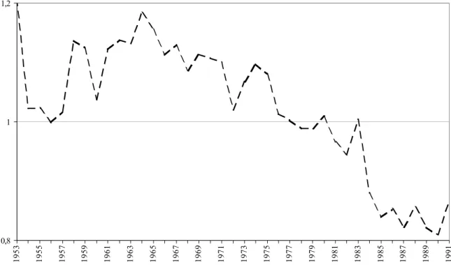
Capacity utilization is, on average, lower than unity (.86) thus indicating under-utilization of the installed capacity. In this respect, more details can be derived by looking at the CUc estimate over the whole period.12 Figure 1 shows that Italian agriculture moves from over to under utilization around 1980, indicating some underlying structural adjustment in the production structure and investment strategy. This is confirmed by the ratio between the long-run equilibrium and the observed levels of the two stock variables (z*/z) (table 1). While physical capital is, on average, scarce thus over-utilized, family labour is always in excess, particularly in the second part of the observed period. Therefore, beyond relative prices movement, both the constant decline of family labour and the constant growth of investment in physical capital in Italian agriculture can be interpreted as the quasi-fixed inputs adjustment to long-run optimal levels.
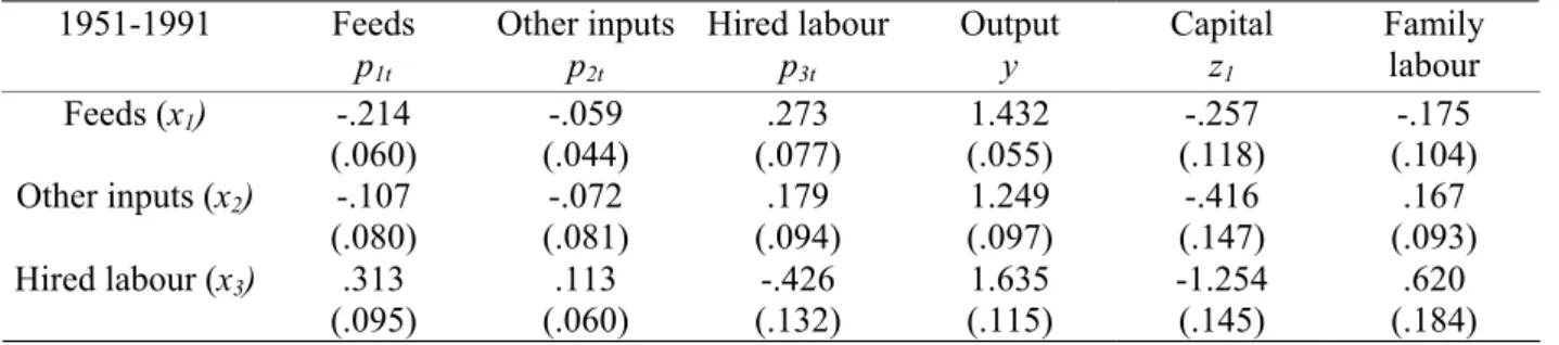
A first look at variable input elasticities in Table 2 reveals that, on the whole, input use is much more responsive to output fluctuations than to prices. Hence, short-run changes in factor proportions are mainly determined by output expansion. Own- and cross-price elasticities indicate that coefficients are accurately estimated and all are smaller than unity, which suggests a rather rigid structure in the short-run. Direct responses of feeds (-.21) and especially of other inputs (-.07) are comparatively low. The own-price elasticity of hired labour (-.43) shows a relatively higher degree of responsiveness. Table 3 reports Morishima elasticities of substitution. The Morishima elasticies are particularly appropriate here since they depend on specific input price changes. They measure how much the input ratio Xi/Xj changes as the price of Xj increases (Celikkol and Stefanou, 1999). Therefore, two inputs are substitute when the respective Morishima elasticity is >0. Table 3 clearly indicates that all variable inputs are substitute; only feeds and other inputs behave as very slight complements in the eighties. Again, elasticities of substitution involving hired labour are by large the highest.
In general, a unit increase in output has a more than proportional effect on the variable inputs, with a relatively stronger impact on hired labour (1.64). Purchased feeds adjust consistently to both fixed inputs, while the signs of other inputs and hired labour adjustments depend upon which stock is changing. In particular, capital is a strong substitute for hired labour (-1.25) and, with a decreasing intensity, for other input (-.42) and purchased feeds (-.26). Finally, family labour substitutes for purchased feeds (-.17) and behaves as complement of the remaining two variable inputs. Most of these adjustments are significant and their absolute values are well above the range of price effects (Esposti and Pierani, 2003b).
Technical change
Technical change is represented by two separate terms: (type II) price-induced technical change is depicted by lagged price impact on input demand; (type I) autonomous technical change is represented by the conventional time trend. Table 1 shows that the latter is indeed negligible and not statistically different from zero. This holds in the whole period and, despite the quadratic splines, quite homogenously in all the sub-periods with a maximum, but still not significant, observed in the sixties with just a 1,4% technical change rate. Since a significant autonomous technical progress has been observed in previous studies on Italian agriculture (Esposti and Pierani, 2003b), this would suggest that type II technical change here takes over most of what was previously attributed to type I (table 5).
With regard to type II technical change it is of particular interest to notice (table A1) that the Koyck constant (λ) is positive and significantly different from 0, thus confirming that the infinite lag structure representing price-inducement is accepted by the data. The estimated value (.540) is lower than that reported in P-S (.695). This seems relevant in terms of the economic interpretation of the price-inducement mechanism. Within this geometrically declining pattern, λ represents the rate of decline, (1-λ) the speed of adjustment and λ/(1-λ) the mean lag. Thus, our results would suggest a little lower rate of decline and mean lag with respect to P-S. If the price lag structure is aimed at
12 CUc indicates the dual measure of capacity utilization. It is derived from the fixed-inputs utilization
mimicking an underlying process of R&D adjustment, this result would imply a shorter effect of R&D over time; that is, R&D investments more oriented toward applied or development activities rather than basic research. This finding supports previous evidence on Italian agriculture (Esposti, 2002; Esposti and Pierani, 2003a).
Overall, the lagged price-induced innovation responses of input demand in Table 4 are well behaved (e.g, own price elasticities are negative), their absolute values are much smaller than the current price elasticities but, unfortunately, have large standard errors in most instances. Hence the discussion of results has to be taken with some caution. The signs of the lagged responses are consistent with the current price counterparts, revealing that, according to expectations, the induced technological innovations have added to the current price substitution effects, during the investigation period.
The role played by this type II technical change in Italian agriculture emerges in table 5, which decomposes the input biases, that is the change in inputs cost share, in the five effects discussed above. These distortion measures, also adopted by Celikkol and Stefanou (1999) and originally proposed by Binswanger (1974), are particularly appropriate to detect the direction of technical change in a multifactor context. It must be noticed that particular attention has to be paid to the interpretation of these biases. Since they measure the change of share on total cost, variable input biases do not sum up to 0, as usually occurs in the long-run context when all inputs are variable. It follows that the sign and magnitude of the different biases in table 5 have to interpreted in relative terms, that is comparing different biases among them for the same input, or comparing the same effect (bias) across the variable inputs.
Three effects of table 5 are not related to technical change. They just measure pure price substitution, the expansion (output) effect and the utilization effect, that is generated by changes in the fixed inputs stock endowment. These biases provide the same qualitative information, though in a different form, already observed in the elasticities commented above. However, the comparison among non-technological change biases also indicates how the utilization effect is the greatest, in absolute term, for all inputs: for other inputs and hired labour the highest effect is generated by change in the capital stock, while for feeds the major role is played by family labour. This supports the idea that disregarding the quasi-fixity of some inputs, and thus the degree of utilization of the installed capacity, may significantly upset the results. The adoption of a restricted cost function thus seems appropriate in this respect.
The last two effects reported in table 5 deal with type I and type II technical change biases, respectively. Results suggest some interesting interpretation on how technical change took form in the last decades in Italian agriculture. First of all, they confirm that type I (autonomous) technical change is indeed negligible not only in terms of overall productivity growth but also in terms of input biases. For no input this effect is relevant in magnitude and it is generally lower than all the other effects. Much more relevant is the role played by type II (price-induced) technical change in determining input biases and this confirms the evidence emerged in Celikkol and Stefanou (1999) while contrasts with results reported by P-S.
Price-inducement is confirmed by the estimated
η
Cjwhose negative and statistical significant values demonstrate that an increase in price generates, after some years, a cost-reducing technical change. Although the lagged prices always generate positive biases, it must be noticed that for all variable input the effect of the own price is the lowest, and this is consistent with the idea that, relatively to other prices, the own price change has the lowest input-using effect. Moreover, change in hired labour price induces feeds-using technical change, as well as change in other inputs price, whereas change in feeds price induces haired labour using technical change.Some final remarks
This paper presents an adaptation of the model proposed by P-S to the analysis of priced-induced technical change in Italian agriculture and within a short-run equilibrium framework. The approach is inspired to the theoretical contributions by Fulginiti (1994) and Paris and Caputo (1995; 2001; 2004), and aims to contribute to the renewed interest on the induced innovation hypothesis emerged in the recent empirical literature.
The main novelty concerns, on the one hand, the sectoral context. Previous works (Celikkol and Stefanou, 1999; P-S) did not focused on the agricultural case, though, indeed, the inducement hypothesis traditionally finds major attention just in the farm sector. On the other hand, however, we try to take a step forward with respect to P-S in the direction of a more accurate representation of the adjustment processes over time. By adopting a short-run specification, both technology adjustment and quasi-fixed inputs adjustment occur in passing from the short-run to the medium-run and, then, long-run equilibrium.
Results here presented generally confirm how this method is particularly suitable to test the price-inducement hypothesis and also to provide a whole set of measures highlighting how inducement takes place occurs and how it interacts with other effects affecting input use proportions and adjustment. Moreover, they support the hypothesis that price-inducement really occurred in Italian agriculture in the last decades and that its magnitude is of major relevance with respect to the other effects, particularly autonomous technical change and pure substitution.
Nonetheless, despite the empirical potential and tractability, the adopted approach leaves some questions open also in the interpretation of the results, and they could be matter of future research on this subject. Firstly, as stressed by the works of Paris and Caputo (1995; 2001; 2004), the theoretical implications of the adopted model with particular reference to the economic interpretation of price-inducement have still to be fully understood and developed, while appear sometime neglected in the empirical applications. Secondly, and more on the empirical ground, the inducement mechanism through an empirical specification of the price lag structure have should be empirically tested, rather than imposed ex-ante (the Koyck structure in our application); in addition, the economic interpretation of this lag structure should me more carefully investigated. In fact, it could mimic the usual time pattern over which research activities generate innovations and innovations are adopted; but this pattern can assume quite different and unpredictable forms (Esposti and Pierani, 2003a). Finally, some econometric implications can also emerge from the introduction of lagged input prices in the model; these may actually generate endogeneity problems thus requiring appropriate IV, or GMM, estimators. Recent empirical applications do not seem to have paid enough attention to this possible estimation issue.
Table 1: Selected indicators of growth in Italian agriculture, 1951-1991 (at the sample means – approximated standard errors in parenthesis)
Y +111
Observed growth rate of output
and input use (%) x1 +258
x2 +310
x3 -50
z1 +317
z2 -69
x1 -4.7
Variation of estimated share on
total cost (%) x2 +.9 x3 +4.2 z1 +7.2 z2 -7.6 CUc .863 (.044) Estimated Capacity
Utilization indicators (mean.) z1*/ z1 1.66
z2*/ z2 .46
1951-1991 -.001 (.004)
Estimated autonomous technical
change rate (-εCt) (mean) 1951-1961 -.014 (.013)
1962-1971 .006 (.008)
1972-1981 .006 (.005)
Table 2: Variable input short-run elasticities (at the sample means – approximated standard errors in parenthesis) 1951-1991 Feeds p1t Other inputs p2t Hired labour p3t Output y Capital z1 Family labour Feeds (x1) -.214 (.060) -.059 (.044) .273 (.077) 1.432 (.055) -.257 (.118) -.175 (.104) Other inputs (x2) -.107 (.080) -.072 (.081) .179 (.094) 1.249 (.097) -.416 (.147) .167 (.093) Hired labour (x3) .313 (.095) .113 (.060) -.426 (.132) 1.635 (.115) -1.254 (.145) .620 (.184) Table 3: Morishima short-run elasticities of substitution of variable inputs (at the sample means)
1951-1991 Feeds Other inputs Hired labour
Feeds (x1) .0 .043 .480
Other inputs (x2) .155 .0 .368
Hired labour (x3) .395 .128 .0
Table 4: Lagged-price elasticities of variable input (at the sample means – approximated standard errors in parenthesis) 1951-1991 Feeds p1t-1 ηij Other inputs p2t-1 Hired labour p3t-1 Feeds ρ1t ηij /(1-λ) Other inputs ρ2t Hired labour ρ3t Feeds (x1) -.104 (.057) -.001 (.037) .105 (.067) -.226 (.118) -.002 (.081) .228 (.145) Other inputs (x2) -.006 (.067) -.014 (.077) .020 (.101) -.013 (.146) -.031 (.167) .044 (.219) Hired labour (x3) .107 (.078) .006 (.064) -.113 (.121) .232 (.172) .013 (.139) -.245 (.264) Table 5: Short-run biases of variable inputs (at the sample means)
1951-1991 Feeds (x1) Other inputs (x2) Hired labour (x3)
Pure substitution P1 -.064 -.019 .004 P2 -.020 -.014 -.005 P3 .010 -.004 -.070 Expansion y .069 -.003 .019 Utilization z1 -.012 -.021 -.078 z2 -.114 -.005 .006
Exogenous technical change
t -.007 .002 .005
Price-induced technical change
p1t-1 .020 .022 .055
p2t-1 .022 .007 .016
Figure 1 – Capacity utilization (CUc) over the whole period
References
Ahmad, S. (1966). On the theory of induced innovation. Economic Journal 76: 344-357.
Binswanger, H. (1974). The measurement of technical change biases with many factors of production. American Economic Review 64: 964-976.
Caiumi, A., Pierani, P., Rizzi, P.L. and Rossi, N. (1995). AGRIFIT: una banca dati del settore agricolo (1951-1991). Milano: Franco Angeli.
Celikkol, P. and Stefanou, S.E. (1999). Measuring the impact of price induced innovation on technological progress: application to the U.S. food processing and distribution sector. Journal of Productivity Analysis 12: 135-151.
Chavas, J.P., Aliber, M. and Cox T.L. (1997). An Analysis of the Source and Nature of Technical Change: the Case of U.S. Agriculture. Review of Economics and Statistics 79: 482-492.
Clark, S.J., Klein, K.K and Kerr, W.A. (2003). Fundamental and induced biases in technological change in central Canadian agriculture. Contributed paper presented at the XXV IAAE Conference - Durban, Reshaping agriculture's contributions to society, http://agecon.lib.umn.edu/.
Esposti, R. (1999). Il progresso tecnico agricolo nell’ottica della crescita endogena: esternalità, spillover e spesa pubblica. La Questione Agraria 74: 27-58.
Esposti, R. (2000). The impact of public R&D and Extension expenditure on Italian agriculture. An Application of a Mixed Parametric/Nonparametric Approach. European Review of Agricultural Economics 27: 365-384.
Esposti, R. (2002). Public agricultural R&D design and technological spill-ins. A dynamic model.
Research Policy 31: 693-717.
Esposti, R. and Pierani, P. (2000). Modelling Technical change in Italian Agriculture: a Latent Variable Approach. Agricultural Economics 22: 261-270.
Esposti, R. and Pierani, P. (2003a). Building the Knowledge Stock: Lags, Depreciation, and Uncertainty in R&D Investment and Productivity Growth. Journal of Productivity Analysis 19: 33-58.
Esposti, R. and Pierani, P. (2003b). Public R&D investment and cost structure in Italian agriculture, 1960- 1995. European Review of Agricultural Economics 30: 509-537.
Esposti, R. and Pierani, P. (2003c). R&D, Technology and Productivity Growth in Italian Agriculture, 1963-1991. Cahiers d’Economie et Sociologie Rurales 67: 5-27.
0,8 1 1,2
Esposti, R. and Pierani, P. (2005). Price, Private Demand and Optimal Provision of Public R&D Investment. An application to Italian agriculture, 1960-1995. Empirical Economics 31 (forthcoming).
Fulginiti, L. (1994). Price-conditional technology. Journal of Agricultural and Resource Economics 19: 161-172.
Hayami, Y. and Ruttan, V.W. (1970). Factor prices and technical change in agricultural development: the United States and Japan, 1880-1960. Journal of Political Economy 78: 1115-1141.
Hayami, Y. and Ruttan, V. (1985). Agricultural development. An international perspective. Baltimore: Johns Hopkins University Press.
Hicks, J.R. (1932). The theory of wages. New York: St. Martins.
Khatri, Y. Thirtle, C., and Townsend, R. (1998). Testing the Induced Innovation Hypothesis: An Application to UK Agriculture, 1953-90. Economics of Innovation and New Technology 6: 1-28.
Koppel, B.M. (1995). Induced innovation theory and international agricultural development: A reassessment. Baltimore: Johns Hopkins University Press
Kumbhakar, S.C. (1989). Estimation of technical efficiency using flexible functional form and panel data. Journal of Business and Economics Statistics 7: 253-258.
Lansink, A.O., Silva, E. and Stefanou, S.E. (2000). Decomposing Productivity Growth Allowing Efficiency Gains and Price-Induced Technical Progress. European Review of Agricultural Economics
27: 497-518.
Lasserre, P. and Ouellette, P. (1991). The measurement of productivity and scarcity rents: the case of asbestos in Canada. Journal of Econometrics 48: 287-312.
Machado, F.S. (1995). Testing the Induced Innovation Hypothesis Using Cointegration Analysis.
Journal of Agricultural Economics 46: 349-360.
Morrison, C.J. (1988). Quasi-Fixed Inputs in U.S. and Japanese Manufacturing: A Generalized Leontief Restricted Cost Function Approach. Review of Economics and Statistics 70: 275-287.
Olmstead, A.L., Rhode, P. (1993): Induced Innovation in American Agriculture: A Reconsideration. Journal of Political Economy 101: 100-118.
Paris, Q. and Caputo, M.R. (1995). The rhetoric of duality. Journal of Agricultural and Resource Economics 20: 195-214
Paris, Q. and Caputo, M.R. (2001): Price-induced technical progress and comparative statics.
Economics Bulletin 15: 1-8.
Paris, Q. and Caputo, M.R. (2004). An atemporal microeconomic theory and an empirical test of price induced technical progress. Working Paper No. 04-009, Department of Agricultural and Resource Economics, University of California, Davis.
Peeters, L. and Surry, Y. (2000). Incorporating price-induced innovation in a Symmetric Generalized McFadden cost function with several outputs. Journal of Productivity Analysis 14: 53-70.
Pierani, P. and Rizzi, P.L. (2003). Technology and Efficiency in a Panel of Italian Dairy Farms: An SGM Restricted Cost Function Approach. Agricultural Economics 29: 195-209.
Pierani, P. and Rizzi, P.L. (1994). Equilibrio di breve periodo, utilizzazione della capacità e
produttività totale dei fattori nell’agricoltura italiana (1952-1991). Discussion Paper, 13,
Dipartimento di Economia Politica, Siena.
Salem, S. (1998). Causality between TFP, R&D and prices: unconditional and conditional linear feedback. Paper presented at the AAEA Meeting, Nashville (Tennessee), August 8-11.
Sunding, D. and Zilberman, D. (2001). The agricultural innovation process: research and technology adoption in a changing agricultural sector. In: Gardner, B.L:,, Rausser, G.C: (eds.):
Handbook of Agricultural Economics. Vol. 1a. Amsterdam: North-Holland, 207-261.
Thirtle, C., Schimmelpfennig, D.E. and Townsend, R. (2002). Induced Innovation in United States Agriculture, 1880-1990: Time Series Tests and an Error Correction Model. American Journal of Agricultural Economics 84: 598-614.
Thirtle, C., Townsend, R. and van-Zyl, J. (1998). Testing the Induced Innovation Hypothesis: An Error Correction Model of South African Agriculture. Agricultural Economics 19: 145-57.
Thirtle, C. (1985). The microeconomic approach to induced innovation: a reformulation of the Hayami and Ruttan model. Manchester School of Economic and Social Studies 53: 263-279.