Data-driven Channel Learning for Next-generation Communication Systems

(1)

Data-driven Channel Learning for

Next-generation Communication Systems

A DISSERTATION

SUBMITTED TO THE FACULTY OF THE GRADUATE SCHOOL OF THE UNIVERSITY OF MINNESOTA

BY

Donghoon Lee

IN PARTIAL FULFILLMENT OF THE REQUIREMENTS FOR THE DEGREE OF

DOCTOR OF PHILOSOPHY

Prof. Georgios B. Giannakis, Advisor

(2)

c

(3)

Acknowledgments

First and foremost, my deepest gratitude goes to my advisor Prof. Georgios B. Gian-nakis. I would like to thank him for giving me a great opportunity to be a member of the SPiNCOM research group, as well as a student of the University of Minnesota, Twin Cities. Without his guidance and insightful suggestions, this thesis would never been completed.

I would like to extend my appreciation to collaborators during my Ph.D. years, Prof. Seung-Jun Kim and Prof. Daniel Romero. Their vast knowledge and insight helped lay a cornerstone for this thesis. Special thanks go to Prof. Mostafa Kaveh, Prof. Mehmet Ak¸cakaya, and Prof. Rui Kuang who agreed to serve as my thesis committee. Thanks also go to a number of other professors in the departments of Electrical Engineering and Computer Science, whose graduate level courses provided me with the necessary background to embark on this area of research.

I also would like to credit current and former members of the SPiNCOM research group for all the good times in Minnesota: Prof. Emiliano Dall’Anese, Prof. Gon-zalo Mateos, Prof. Juan Andr´es Bazerque, Prof. Antonio G. Marqu´es, Prof. Vassilis Kekatos, Prof. Yu Zhang, Dr. Morteza Mardani, Prof. Nasim Soltani, Dr. Brian Baingana, Dr. Dimitris Berberidis, Dr. Fatemeh Sheikholeslami, Dr. Panagiotis Tra-ganitis, Dr. Gang Wang, Prof. Tiany chen, Prof. Yanning Shen, Dr. Liang Zhang, Prof. Jia Chen, Dr. Athanasios Nikolakopoulos, Dr. Qin Lu, Alireza Sadeghi, Georgios Karanikolas, Meng Ma, Vassilis Ioannidis, Bing Cong, Elena Ceci, and Seth Barrash; as well as my friends and colleagues from the Digital Technology Center and the Univer-sity of Minnesota: Charilaos Kanatsoulis, Agoritsa Polyzou, Ioanna Polyzou, Andreas Katis, Maria Kalantzi, Dr. Vasileios Kalantzis, Dr. Dimitrios Zermas, Dr. Panagio-tis Stanitsas, Nikolaos Stefas, Nikos Kargas, Dr. Mohit Sharma, Dr. Shaden Smith,

(4)

Dr. Bo Yang, Dr. Ahmed Zamzam, Faisal Almutairi, Ancy Tom, Dr. Daehan Yoo, Dr. Sehyun Hwang, Prof. Daeha Joung, Prof. Song Min Kim, Dr. Hyungjin Choi, Dr. Chanjoon Lee, Gyubaek Choi, Seonmo Kim, Jeehwan Song, Minsu Kim, Gyusung Park, Taejoon Byun, and Jungseok Hong.

Last but not the least, I am very grateful to my family: my parents Jin Seung Lee and Hawja Yoon, my parents-in-law Sung Won Kim and Kyeong Ok Cha, my grand parents Hee Duk Lee and Junghee Kang, my dear brother Juwon Lee, for their love and support throughout my life. Su, my one and only, I would never make this without you. Thank you for always being next to me.

Donghoon Lee, Minneapolis, October, 2019.

(5)

Dedication

This dissertation is dedicated to Su and Lana for their unconditional love and support.

(6)

The turn of the decade has trademarked the ‘global society’ as an information so-ciety, where the creation, distribution, integration, and manipulation of information have significant political, economic, technological, academic, and cultural implications. Its main drivers are digital information and communication technologies, which have resulted in a “data deluge”, as the number of smart and Internet-capable devices in-creases rapidly. Unfortunately, establishing information infrastructure to collect data becomes more challenging particularly as communication networks for those devices be-come larger, denser, and more heterogeneous to meet the quality-of-service (QoS) for the users. Furthermore, scarcity in spectral resources due to an increased demand for mobile devices urges the development of a new methodology for wireless communications possi-bly facing unprecedented constraints both on hardware and software. At the same time, recent advances in machine learning tools enable statistical inference with efficiency as well as scalability in par with the volume and dimensionality of the data. These consid-erations justify the pressing need for machine learning tools that are amenable to new hardware and software constraints, and can scale with the size of networks, to facilitate the advanced operation of next-generation communication systems.

The present thesis is centered on analytical and algorithmic foundations enabling statistical inference of critical information under practical hardware/software constraints to design and operate wireless communication networks. The vision is to establish a unified and comprehensive framework based on state-of-the-art data-driven learning and Bayesian inference tools to learn the channel-state information that is accurate yet efficient and non-demanding in terms of resources. The central goal is to theoretically, algorithmically, and experimentally demonstrate how valuable insights from data-driven learning can lead to solutions that markedly advance the state-of-the-art performance on inference of channel-state information.

To this end, the present thesis investigates two main research thrusts: i) channel-gain cartography leveraging low-rank and sparsity; and ii) Bayesian approaches to channel-gain cartography for spatially heterogeneous environment. The aforementioned research

(7)

munication networks. Potential of the proposed algorithms is showcased by rigorous theoretical results and extensive numerical tests.

(8)

List of Tables

3.1 Reconstruction error atT = 130 and computational complexity per iter-ation. . . 28 4.1 Hyper-hyperparameters ofθ for synthetic tests. . . 51 4.2 True θ and estimated ˆθ via Alg. 7 (setting of Figs. 4.5c and 4.5d); and

non-adaptive Bayesian algorithm (setting of Figs. 4.5e and 4.5f ) averaged over 20 independent Monte Carlo runs. . . 53 4.3 Hyper-hyperparameters ofθ for real data tests. . . 56 4.4 Estimated ˆθvia benchmark algorithm (setting of Figs. 4.10g and 4.10h);

Alg. 7 (setting of Figs. 4.10c and 4.10d); and non-adaptive Bayesian algorithm (setting of Figs. 4.10e and 4.10f), averaged over 20 independent Monte Carlo runs. . . 59 5.1 Hyper-parameters of θf for synthetic data tests. . . 76

5.2 Trueθand estimated ˆθvia Alg. 9 (setting of Fig. 5.4c); and non-adaptive VB algorithm (setting of Fig. 5.4e) averaged over 20 independent MC runs. 78 5.3 Estimated ˆθ via benchmark algorithm (setting of Fig. 5.7i); Alg. 9

(set-ting of Fig. 5.7e); and non-adaptive VB algorithm (set(set-ting of Fig. 5.7g), averaged over 20 independent MC runs. . . 83

(12)

List of Figures

1.1 Global mobile data traffic and year-on-year growth [23]. . . 2

1.2 Spatial spectrum opportunity of a CR, obtained via (a) a path-loss only model; and (b) a channel-gain map. . . 6

2.1 Illustration of channel-gain maps: (a) local; and (b) global maps. . . 9

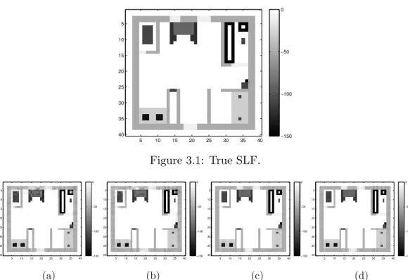
3.1 True SLF. . . 27

3.2 Reconstructed SLFs Fb via batch algorithms: (a) BCD (T = 130, N = 52); (b) APG (T = 130, N = 52); (c) BCD (T = 260, N = 73); and (d) APG (T = 260, N = 73). . . 27

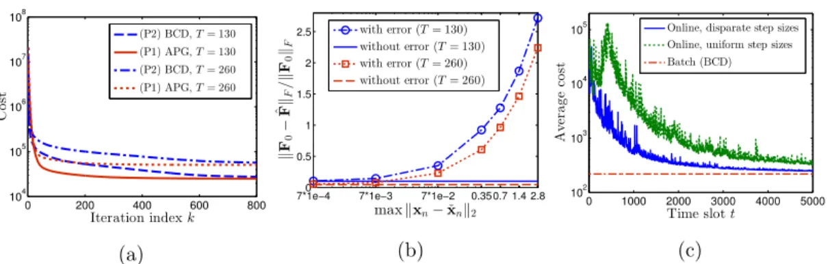
3.3 SLF reconstruction using the batch and online algorithms. (a) Cost ver-sus iterations (batch). (b) Reconstruction error verver-sus CR location error (batch). (c) Average cost over time slots (online). . . 28

3.4 Reconstructed SLFsFb by the online algorithm with (a)-(b) ¯η (t) P = ¯η (t) Q = 300 and ¯η(_Et)= 10; and (c)-(d) ¯η_P(t) = ¯η_Q(t)= ¯η(_Et)= 300. . . 29

3.5 (a)-(b) True SLFs F(₀t) and (c)-(d) reconstructed SLFs Fb(t) at different time slots. . . 29

3.6 Configuration of the testbed withN = 80 sensor locations marked with crosses. . . 30

3.7 Reconstructions by the proposed batch algorithm in Alg. 1. . . 30

3.8 Reconstructions by the ridge-regularized LS. . . 31

3.9 Reconstructions by the proposed online algorithm in Alg. 2. . . 31

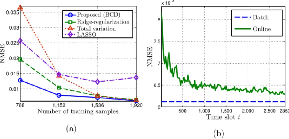
3.10 NMSE of channel gain prediction by (a) the batch; and (b) online algo-rithms. . . 32

4.1 Four-connected MRF with z(˜xi) marked red and its neighbors in N(˜xi) marked blue. . . 37

(13)

tography, together with the measurement model for sensors located at (xn,xn0). . . 37

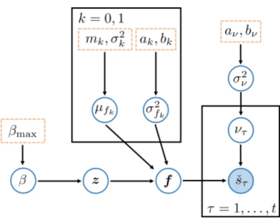
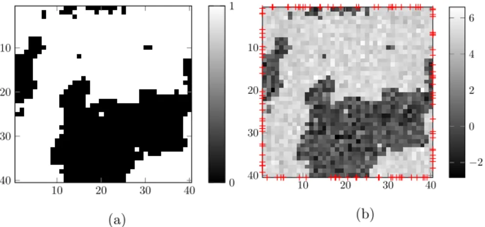
4.3 Graphical representation of the hierarchical Bayesian model with Ising prior for (hyper) parameters (those in boxes are fixed). . . 39 4.4 True fields for synthetic tests: (a) hidden label field Z0 and (b) spatial

loss fieldF0 withN = 120 sensor locations marked with crosses. . . 52

4.5 Estimated SLFs Fb at τ = 15 (with 700 measurements) via (a)

ridge-regularized LS (µf = 8.9×10−4 andCf =I1,600); (b) TV-regularized LS

(µf = 10−12); (c) Alg. 7 through (d) estimated hidden label fieldZb; and

(e) non-adaptive Bayesian algorithm, through (f) estimatedZb. . . 53

4.6 Progression of error in estimation ofz. . . 54 4.7 Reconstruction error vs. noise varianceσ2

ν for (a) the SLFf; and (b) the

hidden label fieldz. . . 54 4.8 True SLFs for (a)τ _{∈ {}0, . . . ,5_}; and (b)τ _{∈ {}6, . . . ,15_}; and estimated

SLFs at (c) τ = 5 (300 measurements); and (d) τ = 15 (700 measure-ments) via Alg. 7. Dynamic objects are marked with dotted circles. . . . 55 4.9 Progression of channel-gain estimation error. . . 56 4.10 Estimated SLFs Fb at τ = 5 (with 1,880 measurements) via (a)

ridge-regularized LS; (b) TV-ridge-regularized LS; (c) Alg. 7 through (d) estimated hidden label field Zb; and (e) non-adaptive Bayesian algorithm, through

(f) estimated Zb, together with one-shot estimates (g) Fb_full and (h) Zb_full

obtained by using the full dataset (with 2,380 measurements) via Alg. 7. 57 4.11 Progression of a mismatch betweenzband zbfull. . . 59

4.12 Estimated shadowing mapsSband corresponding channel-gain mapsGb at

τ = 5 via (a)-(b) ridge-regularized LS (setting of Fig. 4.10a); (c)-(d) TV-regularized LS (setting of Fig. 4.10b); (e)-(f) Alg. 7 (setting of Fig. 4.10c); and (g)-(h) non-adaptive Bayesian algorithm (setting of Fig. 4.10e), with the receiver location atxrx= (10.3,10.7) (ft) marked with the blue cross. 60

5.1 Gauss-Markov-Potts model for channel-gain cartography with K = 3, together with the measurement model for sensors located at (xn,xn0). . 65

(14)

(hyper) parameters (those in dashed boxes are fixed). . . 66 5.3 True fields for synthetic tests: (a) hidden label field Z0 and (b) spatial

loss fieldF0 withN = 200 sensor locations marked with crosses. . . 74

5.4 SLF estimates Fb at τ = 8 (with 1,600 measurements) via; (a)

ridge-regularized LS (µf = 0.015 and Cf = I3,600); (b) TV-regularized LS

(µf = 10−11); (c) Alg. 9 through (d) estimated hidden field Zb; (e)

non-adaptive VB algorithm through (f) Zb; (g) adaptive MCMC algorithm

through (h)Zb; (i) non-adaptive MCMC algorithm through (j)Zb; and (k) b

Ffull and (l) Zb_full obtained by using the full data (with 2,400

measure-ments) via Alg. 9. . . 77 5.5 Progression of estimation error of z versus (a) time τ; and (b) noise

precisionϕν, averaged over 20 MC runs. . . 78

5.6 Progression of channel-gain estimation error. . . 79 5.7 SLF estimates Fb at τ = 5 (with 1,880 measurements) via; (a)

ridge-regularized LS (µf = 0.015 and Cf = I3,600); (b) TV-regularized LS

(µf = 6); (c) adaptive MCMC algorithm in [50] withK= 2 through (d)

estimated hidden fieldZb; (e) Alg. 9 through (f)Zb; (g) non-adaptive VB

algorithm through (h)Zb; and (i)Fb_full and (j)Zb_full obtained by using the

full data (with 2,380 measurements). . . 81 5.8 Progression of a mismatch between ˆz and ˆzfull. . . 82

5.9 Estimated shadowing maps bS and corresponding channel-gain maps Gb

at τ = 5 via (a)-(b) ridge-regularized LS (setting of Fig. 5.7a); (c)-(d) TV-regularized LS (setting of Fig. 5.7b); (e)-(f) adaptive MCMC algo-rithm in [50] withK= 2 (setting of Fig. 5.7c); (g)-(h) Alg. 9 (setting of Fig. 5.7e); and (i)-(j) non-adaptive VB algorithm (setting of Fig. 5.7g); and (k)–(l) benchmark algorithm (setting of Fig. 5.7i), with the receiver location atxrx= (10.3,10.7) (ft) marked with the black cross. . . 84

(15)

Chapter 1

Introduction

1.1 Motivation and Context

Smart and Internet-capable devices have a ubiquitous presence in our daily lives. In the first quarter of 2019, global mobile penetration is 104 percent, bringing the total num-ber of mobile subscriptions to around 7.9 billion. Correspondingly, the global mobile data traffic grew by 82 percent between 2018 and 2019 and reached 32 exabytes (equal to 3.2×1018 _{bytes) per month [23], which is primarily fueled by viewing multimedia}

content at increasingly higher resolution; see the mobile data traffic growth in Fig. 1.1. While there is increasing demand for wireless connectivity, the spectrum particularly between 500 MHz and 3 GHz is limited; and most of defined spectrum bands have al-ready been allocated for governmental and commercial activities. Additionally, growing interest in the Internet of things (IoT) puts a strain on the available unlicensed spectral resources. Provided that the projected number of IoT devices in factories, businesses, and healthcare reaches 200 billion by 2020 [41], the currently available spectrum will be eventually overloaded and considerable interference issues will arise as a result.

Evident scarcity of spectral resources for (un)licensed bands has popularized mainly two different ideas as potential remedies: i) spectrum sharing; and ii) utilization of higher frequencies. As a manifestation of the former, cognitive radio networks (CRNs) have arguably gained center-stage prominence. Cognitive radios (CRs) are a set of devices equipped with cognition capabilities to learn the spatio-temporal and spectral

(16)

Figure 1.1: Global mobile data traffic and year-on-year growth [23].

usage patterns of near by users and networks. Such a level of cognition allows op-portunistic utilization of the unused (un)licensed spectrum via spectrum sensing and dynamic spectrum access while avoiding interference in networks operating over the same band. This is particularly appealing in a recent situation that the licensed RF spectrum is often severely under-utilized depending on the time and location of commu-nication [25]. While spectrum sharing has been proposed for more efficient use of exist-ing spectral resources, utilization of higher frequencies addresses not only the spectral scarcity, but also increasing demand for higher date rates. Millimeter wave (mmWave) communications over the licensed spectrum between 30–300 GHz have recently gained more attention from the standards organization, the Federal Communications Commis-sion (FCC), and academia as a means to bring “5G” cellular systems into the future, while those over the unlicensed spectrum were mainly studied to develop technologies for a personal area network (PAN) to deliver uncompressed high definition (HD) video, or standardized for a wireless local area network (WLAN); see e.g., WirelessHD [92] and IEEE 802.11ad [1], respectively.

While the aforementioned solutions promise more efficient utilization of the spectral resources and faster means of wireless communication, next-generation communication systems face formidable challenges as outlined next.

(17)

C1. Networks are ultra dense and heterogeneous. One differentiator of 5G networks relative to legacy generations (1–4G) is heterogeneity, which is induced by the convergence of “component” networks in various sizes operating over potentially different frequency bands. These so-termed heterogeneous networks (HetNets) are key enablers of 5G systems together with densification of the infrastructure to meet quality-of-service (QoS) expected by users and satisfy different service coverage requirements, provided that seamless interconnections among component networks are guaranteed. While CRs are considered as a key technology to accommodate the HetNets by providing adaptive handover between component networks [43], the successful operation of CRNs hinges critically on channel state information (CSI) over space, time, and frequency to find spectrum holes [47]. However, conventional point-to-point estimation methods such as ray-tracing [87, 93] do not provide feasible solutions for extremely dense and heterogeneous networks.

C2. Differences of mmWave channel relative to sub-6 GHz channel. Com-pared to the channel at sub-6 GHz, the millimeter wave channel shows significantly different characteristics due to the very short wavelength relative to the size of objects located in the propagation environment. This results in high sensitivity of signals to blockages, with consequently pronounced shadowing effects but relatively low diffrac-tion [57]. For example, signal strength can be attenuated as much as 35dB by the human body [54]. Furthermore, the signal propagating over mmWave bands experi-ences higher path-loss than that at sub-6 GHz with omnidirectional antennas since the path-loss is inversely proportional to the wavelength squared by the Friis’ law. In other words, mmWave communications become feasible through either co-siting with existing technologies, or directional transmissions and MIMO techniques with adaptive beamforming, to compensate for severe signal attenuation.

C3. New hardware constraints on massive MIMO for mmWave commu-nication. To implement mmWave communication systems by addressing C2, it is inevitable to adopt MIMO techniques with antenna arrays having between 16 to 256 elements [37], which could be even larger at base stations in cellular networks. For such

(18)

a large number of antenna elements, several hardware constraints arise from a practi-cal point of view. Conventional digital MIMO architectures at sub-6 GHz frequencies (generally with two antenna elements) entail a power amplifier (PA) and an RF chain with analog-to-digital converter (ADC), or digital-to-analog converter (DAC), associ-ated with each antenna on top of all baseband connections. As the number of antenna elements increases, it becomes impractical to pack all these devices on a circuit board with limited space while placing antennas very close to each other to avoid granting lobes. Furthermore, power consumption is another critically limiting factor; e.g, power hungry devices such as ADC or PA consume 15–795 (mW) per antenna [27, 20]. There-fore, implementation of mmWave communications requires z beamforming architecture with low-power consumption while providing a sufficient spatial multiplexing gain by supporting amassive number of antenna arrays.

In this context, the present dissertation will leverage contemporary science and en-gineering tools from diverse disciplines in order to put forth analytical and algorithmic foundations to design and operate modern communication systems.

1.2 Channel-gain Cartography

The abiding goal of this thesis is to jointly address challenges C1–C3 under a prin-cipled machine learning framework. To tackle C1 and C2, we put forth algorithmic innovations for efficient and adaptive learning of global channel-state information for next-generation communication systems via channel-gain cartography. On the other hand, future research directions to address C3 will be discussed in Chapter 6.

Channel-gain cartography is a groundbreaking geostatistics-inspired application por-traying the RF landscape impinging upon arbitrary spatial locations. The most appeal-ing feature of this tool is the non-trivial capability of inferrappeal-ing channel-gain between arbitrary transceiver locations, even where no sensor is deployed, based only on mea-surements collected by a set of collaborating sensing radios. The vision of channel-gain cartography is to utilize the resulting channel-gain atlas for cross-layer design and as-sessment of the system-level performance of wireless networks; and to enhance hand-off, routing, interference management, and resource allocation, without requiring a large number of point-to-point channel estimates over wireless networks.

(19)

Channel-gain cartography leverages the notion of spatial loss fields (SLFs), which are maps quantifying the attenuation experienced by electromagnetic waves in radio frequency (RF) bands at every spatial position. The SLF model is used to estimate shadowing over an arbitrary radio link, and subsequently the associated channel gain as well. This enables construction of a map depicting a landscape of channel-gain from any point to a common end point in the region of interest. Considering that characterization of the propagation environment is critical for obtaining the channel-state information based on situational awareness, more accurate spectrum sensing and aggressive spatial reuse can be expected from utilization of a channel-gain map, instead of adopting a path-loss only model. Fig. 1.2 delineates spatial spectrum opportunity at a secondary receiver marked by a black cross, obtained via the proposed channel-gain map and the path-loss only model. For illustration purposes, the threshold to meet the QoS is set to 60dB and corresponding contour is drawn in red. Apparently, the spatial coverage of the receiver obtained by using the channel-gain map expands more than that by using the path-loss only model. This demonstrates nicely that more aggressive spatial reuse becomes available due to site-specific interference management through the proposed channel-gain map.

Such a non-trivial capability of inferring any-to-any channel-gain can be a key to success of spectrum reuse over HetNets, and co-siting for mmWave communications by enhancing hand-off, routing, and interference management. These considerations motivate the innovative machine learning and Bayesian inference algorithms for channel-gain cartography that will be developed in the following chapters and, accordingly, a significant departure from conventional per-link channel-gain and interference level estimation will be advocated.

1.3 Thesis Outline

The remainder of the thesis is organized as follows.

Chapter 2 reviews channel-gain cartography. The concept of channel-gain cartog-raphy is introduced with its functionality. Prior works including radio tomogcartog-raphy are reviewed as well. Afterwards, the system model and problem statement are presented, which are considered throughout the thesis.

(20)

60 60 60 60 60 0 10 20 20 10 0 [ft] [ft] 50 55 60 65 70 75 80 85 [dB] (a) 60 60 60 60 60 60 0 10 20 20 10 0 [ft] [ft] 50 55 60 65 70 75 80 85 [dB] (b)

Figure 1.2: Spatial spectrum opportunity of a CR, obtained via (a) a path-loss only model; and (b) a channel-gain map.

Chapter 3 puts forth channel-gain cartography leveraging low-rank and sparsity, having as goal to construct a channel-gain map with a relatively small number of mea-surements. The key idea is to postulate that the SLF has a low-rank structure poten-tially corrupted by sparse outliers. Such a model is particularly appealing for urban and indoor propagation scenarios, where regular placement of buildings and walls renders a scene inherently of low-rank, while sparse outliers can pick up the artifacts that do not conform to the low-rank model. We develop an efficient batch algorithm as well as its online version via stochastic approximation (SA) [84, 48]. Performance of the proposed algorithms is evaluated with a rigorous performance analysis and extensive numerical tests on synthetic and real datasets.

Chapter 4 introduces a novel Bayesian framework for channel-gain cartography. To take into account spatial heterogeneity of the propagation environment when learning the SLF, we propose a two-layer Bayesian SLF model based on a binary hidden Markov random field along with Markov chain Mote Carlo (MCMC) methods for inference [30]. Besides accounting for heterogeneous propagation environments, another contribution here is a data-adaptive sensor selection technique, with the goal of reducing SLF uncer-tainty, by cross-fertilizing ideas from the fields of experimental design [26] and active learning [55]. Efficacy of the proposed solution is established through extended synthetic and real data tests.

(21)

Chapter 5 builds on the algorithms and results of Chapter 4, and devises a variational Bayes approach to adaptive Bayesian channel-gain cartography. The aforementioned Bayesian SLF model is generalized first by adopting a K-ary hidden Markov random field, to address a richer class of environmental heterogeneity. Subsequently, variational Bayes (VB) algorithms are developed to provide efficient field estimators at affordable complexity. To bypass a novel but intractable sensor selection criterion, its efficient proxy can be obtained thanks to the availability of an approximate posterior model from the proposed VB algorithm. Numerical tests on synthetic and real data corroborate the effectiveness of the proposed algorithms.

Finally, Chapter 6 presents a concluding discussion of the proposed approaches, along with future research directions.

1.4 Notational Conventions

The following notation is used throughout the subsequent chapters. Bold uppercase (lowercase) letters denote matrices (column vectors). Calligraphic letters are used for sets; In is the n×n identity matrix; 0n denotes an n×1 vector of all zeros, and 0n×n an n×n matrix of all zeros. Operators (·)>, tr(·), σi(·), and λmax(·) represent

the transposition, trace, the i-th largest singular value, and the largest eigenvalue of a matrix, respectively; | · | is used for the cardinality of a set, the magnitude of a scalar, and the determinant of a matrix. R0signifies thatRis positive semidefinite. The `1-norm of X ∈ Rn×n is kXk1 := Pni,j=1|Xij|. The `∞-norm of X ∈ Rn×n is

represented by _kX_k∞ := max{|Xij|:i, j = 1, . . . , n}. For two matrices X,Y ∈ Rn×n,

the matrix inner product is _hX,Y_i := tr(X>Y). The Frobenius norm of matrix Y

is kYkF :=

p

tr(YY>). The spectral norm of Y is kYk := maxkxk2=1kYxk2, and kY_k∗ := P_iσi(Y) is the nuclear norm of Y. For a function h : Rm×n → R, the

directional derivative of h at X ∈ Rm×n _{along a direction} _D _∈ _Rm×n _{is denoted by}

h0(X;D) := limt→0+[h(X+tD)−h(X)]/t. vec(X) produces a column vector x∈Rmn

by stacking the columns of a matrix one after the other (unvec(x) denotes the reverse process). For a vector y_∈Rn and ann_×nweight matrix ∆, the weighted norm of y

(22)

Chapter 2

Channel-gain Cartography

2.1 Preliminaries and Motivation

Conventional acquisition of the channel-state information (CSI) on a per-link basis might become inadequate for emerging wireless technologies, since needs for accounting situ-ational awareness are unrelentingly demanded to accomplish dynamic spectral resource control for spectrum sharing in next-generation communication systems [96, 75, 40].

To meet the demands for tools enabling aggressive and full opportunistic utilization of the unused (un)licensed spectrum, radio frequency (RF) cartography was proposed as an instrumental concept originally for cognitive radios (CRs) [46]. Based on the measurements collected by spatially distributed sensing radios, RF cartography provides tools to construct maps over the space, time, and frequency, portraying a RF landscape in which a CR network is deployed. Notable RF maps that have been proposed include a power spectral density (PSD) map, which acquires the ambient interference power distribution, revealing the crowded regions that CR transceivers need to avoid [6]; and a channel-gain (CG) map, which delineates the spatial distribution of channel-gain in a given geographical region through a collaborative network of CRs, allowing CR networks to perform accurate spectrum sensing and aggressive spatial reuse [47]. The present thesis focuses on channel-gain cartography.

Given channel-gain measurements from sensing radios at known locations in a region of interest, the goal of channel-gain cartography is to estimate or predict channel-gain from any point to a deployed radio, which is henceforth termed as a local CG map; as

(23)

(a) (b)

Figure 2.1: Illustration of channel-gain maps: (a) local; and (b) global maps.

well as that of an arbitrary wireless link from any point to any other point in space, (i.e., links not having communication ending points in common with the links between existing sensing radio pairs), which constitute a so-termed global CG map: local and global CG maps are illustrated in Fig. 2.1. The vision of channel-gain cartography is to utilize resultant channel-gain atlas for cross-layer design and assessment of the system-level performance of wireless networks; and to provide the vital information for interference management, resource allocation, and spectrum sensing. It is also notable that channel-gain cartography relies on incoherent measurements containing no phase information, e.g., the received signal strength (RSS). Such simplification saves costs for synchronization needed to calibrate phase differences among waveforms received at different sensors.

The key premise behind channel-gain cartography is that spatially close radio links exhibit similar shadowing due to the presence of common obstructions. This shadowing correlation is related to the geometry of objects present in the area that waves prop-agate through [71, 2]. As a result, shadowing is modeled as the weighted line integral of the underlying two-dimensional spatial loss field (SLF), which is a map quantify-ing the attenuation experienced by electromagnetic waves in RF bands at every spatial position [71]. The weights in the integral are determined by a function depending on the transmitter-receiver locations [71, 33, 82], which models the SLF effect on shad-owing over a link. Inspired by this SLF model, linear interpolation techniques such as kriging were further employed to estimate shadowing based on spatially correlated mea-surements [18], while spatio-temporal dynamics were tracked via Kalman filtering [47]. Instead of relying on heuristic criteria to choose the weight function, [82] provides blind

(24)

algorithms to learn the weight function using a non-parametric kernel regression, while estimating the SLF via regularized least-squares (LS) methods. Note that another body of work leveraging the SLF model is radio tomographic imaging (RTI) [91]. Benefiting from the ability of RF waves to penetrate physical structures such as trees and buildings, RTI provides a means of device-free passive localization [94, 97], and has found diverse applications in disaster response for e.g., detecting individuals trapped in buildings or smoke [90]. To detect locations of changes in the propagation environment, one can use the difference between the SLF across consecutive time slots [91, 89]. To cope with multipath in a cluttered environment, multi-channel measurements can be utilized to enhance localization accuracy [44]. Although these are calibration-free approaches, they cannot reveal static objects in the area of interest. It is also possible to replace the SLF with a label field indicating presence (or absence) of objects in motion on each voxel [90], and leverage the influence that moving objects on the propagation path have, on the variance of a RSS measurement. On the other hand, the SLF itself was reconstructed in [32, 33] to depict static objects in the area of interest, but calibration was necessary by using extra measurements (e.g., collected in free space). One can avoid extra data for calibration by estimating the SLF together with pathloss components [8, 82]. Exploit-ing the sparse occupancy of the target objects in a monitored area, sparsity-leveragExploit-ing algorithms for constructing obstacle maps were also developed [66, 45, 65].

The overarching contribution of the present thesis is to develop algorithmic founda-tions for effective data-driven channel learning by capitalizing on the inherent structure of measurement data, rather than relying heavily on the physics of RF propagation. RF propagation environment is particularly taken into consideration as the prior informa-tion to learn the shadowing model, inspired by a fact that absorpinforma-tion captured by the SLF allows one to discern objects located in the area of interest. We propose two SLF models: i) a low-rank plus sparse matrix model [16, 24, 59]; and ii) a hidden Markov random field (MRF) model [38]. The former is appealing for urban and indoor propaga-tion scenarios, where regular placement of buildings and walls renders a scene inherently of low rank, while sparse outliers can pick up the artifacts that do not conform to the low-rank model. On the other hand, the latter is useful when the propagation environ-ment is spatially diverse due to a combination of free space and objects in different sizes and materials, which subsequently induces statistical heterogeneity in the SLF. Efficient

(25)

solution methods leveraging aforementioned SLF models will be developed, and their efficacy is shown through extensive synthetic and real data tests.

2.2 System Model and Problem Statement

Consider a set of sensors deployed over a two-dimensional geographical area A ⊂ R2_.

After averaging out small-scale fading effects, the channel-gain measurement over a link between a transmitter located at x ∈ A and a receiver located at x0 ∈ A can be represented (in dB) as

g(x,x0) =g0−γ10 log10d(x,x

0

)−s(x,x0) (2.1)

whereg0 is the path gain at unit distance;d(x,x0) :=kx−x0kis the Euclidean distance

between the transceivers at x and x0; γ is the pathloss exponent; and s(x,x0) is the attenuation due to shadow fading.

A tomographic shadow fading model is [71, 33, 51]

s(x,x0) =

Z

A

w(x,x0,x˜)f(˜x)dx˜ (2.2)

where f : A → R denotes the spatial loss field (SLF) capturing the attenuation at location ˜x, and w : _{A × A × A →} R is a weight function describing how the SLF at ˜

x contributes to the shadowing experienced over the link x–x0. Typically, w confers a greater weight w(x,x0,x˜) to those locations ˜xlying closer to the link x–x0. Examples of the weight function include the normalized ellipse model [89]

w(x,x0,x˜) :=    1/pd(x,x0₎_, _if_d₍_x_,_x_˜_{) +}_d₍_x0_,_x_˜₎_{< d}₍_x_,_x0_{) +}_λ/₂ 0, otherwise (2.3)

where λ >0 is a tunable parameter. The value of λis commonly set to the wavelength to assign non-zero weights only within the first Fresnel zone. It is worth to mention that the weight function can be learned via a non-parametric kernel regression, instead of relying on on heuristic criteria to choose the weight function; see [82] for details. In

(26)

practice, the integral in (2.2) is approximated by a finite sum as s(x,x0)_'c Ng X i=1 w(x,x0,x˜i)f(˜xi) (2.4) where _{x˜i} Ng

i=1 is a grid of points over A and c is a constant that can be set to unity

without loss of generality by absorbing any scaling factor inf. Clearly, (2.4) shows that

s(x,x0) depends on f only through its values at the grid points.

The model in (2.2) describes how the spatial distribution of obstructions in the propagation path influences the attenuation between a pair of locations. The usefulness of (2.2) is twofold: i) as f represents absorption across space, it can be used for imag-ing; and ii) once f and w are known, the gain between any two points x and x0 can be recovered through (2.1) and (2.2), which is precisely the objective of channel-gain cartography.

All in all, the objective of channel-gain cartography is tantamount to estimating

f. To this end, N sensors located at{x1, . . . ,xN} ∈ Acollaboratively obtain

channel-gain measurements. At time slot τ, the radios indexed byn(τ) andn0(τ) measure the channel-gain ˇgτ :=g(xn(τ),xn0₍_τ₎) +ν_τ by exchanging training sequences known to both

transmitting and receiving radios, where n(τ), n0(τ)∈ {1, . . . , N} and ντ denotes

mea-surement noise. It is supposed that g0 and γ have been estimated during a calibration

stage. After subtracting known components from ˇgτ, the shadowing estimate is found

as

ˇ

sτ :=g0−γ10 log10d(xn(τ),xn0₍_τ₎)−ˇg_τ

=s(xn(τ),xn0₍_τ₎)−ν_τ. (2.5)

Having available ˇst:= [ˇs1, . . . ,sˇt]>∈Rtalong with the known set of links{(xn(τ),xn0₍_τ₎)}t_τ₌₁

and the weight function w at the fusion center, the problem is to estimatef, and thus

f := [f(˜x1), . . . , f(˜xNg)]

> _∈ _RNg _{using (2.4). Once ˆ}_f _{is obtained, shadowing and}

subsequently channel-gain across any link x–x0 can be estimated via (2.4) and (2.1) as

ˆ s(x,x0) = Ng X i=1 w(x,x0,xi˜ ) ˆf(˜xi) (2.6)

(27)

ˆ

(28)

Chapter 3

Channel-gain Cartography

leveraging Low-rank and Sparsity

A task of channel-gain cartography is well-motivated to benefit operation of cognitive radio networks (CRNs) by providing a means of site-specific interference management and subsequently, spectrum sensing. Although more sophisticated methodologies for channel modeling do exist including ray tracing [87, 93] to serve the same purpose, the computational cost and requirements on various structural/geometric prior information may hinder their use in CR applications. Capitalizing on experimentally validated notion of the spatial loss field (SLF) [2], we will provide a computationally efficient solution by leveraging the inherent structure of data, rather than relying heavily on the physics of radio frequency (RF) signal propagation.

Our work interpolates the channel gains based on the SLF reconstructed from a small number of measurements using a low-rank and sparse matrix model. The key idea is to postulate that the SLF has a low-rank structure potentially corrupted by sparse outliers. Such a model is particularly appealing for urban and indoor propagation scenarios, where regular placement of buildings and walls renders a scene inherently of low rank, while sparse outliers can pick up the artifacts that do not conform to the low-rank model. While it is true that urban and indoor environments have distinct profiles due to the different scales and density of obstacles, our data model can capture the structural regularity of obstacles, possibly at different scales, as validated through

(29)

synthetic and real data examples in Section 3.3. The sparse term helps robustify this model by filtering out the measurements that do not conform to the low-rank structure. This is essentially the idea behind robust principal component analysis [16], which is a powerful data model that has been used widely.

In fact, since a shadowing measurement is modeled as a linear tomographic mea-surement of the SLF, the map recovery task reduces to an instance of compressive principal component pursuit (CPCP) [95]. In general, the CPCP problem recovers the low-rank and sparse matrices from a small set of linearly projected measurements. Our algorithms are applicable to this general problem class.

We develop efficient batch and online algorithms for channel-gain cartography. By replacing the nuclear norm-based regularizer with a bi-factorization surrogate, a block coordinate descent (BCD) algorithm becomes available to avoid costly singular value decomposition (SVD) per iteration. Although the resulting optimization problem is non-convex, the batch solver can attain the global optimum under appropriate conditions. For the online algorithm, a stochastic successive upper-bound minimization strategy is adopted, leading to a stochastic gradient descent (SGD) update rule, which enjoys low computational complexity. The iterates generated by the online algorithm are provably convergent to the stationary point of the batch problem.

3.1 Channel-gain estimation using Low-rank and Sparsity

The goal of the present section is to estimate the SLF by leveraging its inherent low-rank and sparse attribute. To this end, let matrix F := unvec(f) _∈ _RNx×Ny _denote

the SLF, sampled by the Nx-by-Ny grid, where Ng = NxNy. Let further define w(_nnt)0 := [w(x_n₍_t₎,x_n0₍_t₎,x˜₁), . . . , w(x_n₍_t₎,x_n0₍_t₎,x˜_N_g)]> ∈ RNg. Then, the weight

ma-trixW(_nnt)0 := unvec(w (t)

nn0)∈RNx×Ny corresponding to linkx_n₍_t₎–x_n0₍_t₎is constructed in

similar manner. Subsequently, the shadow fading over link xn(t)–xn0₍_t₎ in (2.4) can be

expressed as a linear projection of the SLF given by

s(x_n₍_t₎,x_n0₍_t₎)' hW(t)

nn0,Fi. (3.1)

In the following sections of Chapter 3, the measurement model in (3.1) will be specifically considered.

(30)

3.1.1 CPCP Problem formulation

The low-rank plus sparse structure has been advocated in various problems in machine learning and signal processing [16, 24, 59]. Low-rank matrices are effective in capturing slow variation or regular patterns, and sparsity is instrumental for incorporating robust-ness against outliers. Inspired by these, we postulate that Fhas a low-rank-plus-sparse structure as

F=L+E (3.2)

where matrix L is low-rank, and E is sparse. This model is particularly attractive in urban or indoor scenarios where the obstacles often possess regular patterns, while the sparse term can capture irregularities that do not conform to the low-rank model.

Redefine ˇs(_nnt)0 := ˇs(x_n₍_t₎,x_n0₍_t₎) for brevity. Let M(t) be the set of links, for which

channel gain measurements are made at timet, and collect those measurements in vector ˇ

s(t) _∈_R|M(t)_|

. Toward estimating F(t) _{that obeys (3.2), consider the cost}

c(t)₍_L_,_E_{) :=} 1 2 X (n,n0₎_∈M(t) hW_nn(t)0,L+Ei −sˇ (t) nn0 2 (3.3)

which fits the shadowing measurements to the model. Then, withT denoting the total number of time slots taking measurements, we adopt the following optimization criterion

(P1) min L,E∈_RNx×Ny T X τ=1 βT−τhc(τ)(L,E) +µLkLk∗+µEkEk1 i (3.4)

whereβ_∈(0,1] is the forgetting factor that can be optionally put in to weigh the recent observations more heavily. The nuclear norm regularization term promotes a low-rank

L, while the`1-norm encourages sparsity inE. ParametersµLandµEare appropriately

chosen to control the effect of these regularizers. Conditions for exact recovery through a related convex formulation in the absence of measurement noise can be found in [95]. Problem (3.4) is convex, and can be tackled using existing efficient solvers, such as the interior-point method. Once the optimal Lb and Eb are found, the desired Fb is

ob-tained asFb =Lb+Eb. However, the general-purpose optimization packages tend to scale

(31)

often employ costly SVD operations iteratively [95]. Furthermore, such an algorithm might not be amenable for an online implementation. Building on [58] and [81], an efficient solution is proposed next with reduced complexity.

3.1.2 Efficient batch solution

Without loss of generality, consider replacingLwith the low-rank productPQ>, where

P_∈RNx×ρ_and _Q_∈RNy×ρ_{, and}_ρ_{is a pre-specified overestimate of the rank of}_L_{. It is}

known that (e.g., [81])

kLk∗ = min P,Q 1 2 kPk 2 F +kQk2F subject to L=PQ>. (3.5)

Thus, a natural re-formulation of (3.4) is (see also [58])

(P2) min P,Q,Ef(P,Q,E) := T X τ=1 βT−τhc(τ)(PQ>,E) +µL 2 kPk 2 F +kQk2F +µEkEk1 i . (3.6)

Instead of seeking the NxNy entries of L, the factorization approach (3.6) entails only

(Nx+Ny)ρunknowns, thus reducing complexity and memory requirements significantly

when ρmin_{Nx, Ny}. Furthermore, adoption of the separable Frobenius norm

regu-larizer in (P2) comes with no loss of optimality as asserted in the following lemma.

Lemma 1: If {Lb,Eb} minimize (P1) and we choose ρ ≥ rank(Lb), then, (P2) is

equivalent to (P1) at the minimum.

Proof: It is clear that the minimum of (P1) is no larger than that of

min P,Q,E T X τ=1 βT−τh_c(τ)₍_PQ>_,_E_{) +}_µ LkPQ>k∗+µEkEk1 i (3.7)

since the search space is reduced by the reparameterization L = PQ> with ρ ≤

min_{Nx, Ny}. Now (3.5) implies that the minimum of (3.7) is no larger than that

of (P2). However, the inequality is tight since the objectives of (P1) and (P2) are identical for E := Eb, P := UbΣb

1/2

, and Q := VbΣb

1/2

(32)

Consequently, (P1) and (P2) have identical costs at the minimum.

Although (P1) is a convex optimization problem, (P2) is not. Thus, in general, one can obtain only a locally optimal solution of (P2), which may not be the globally optimal solution of (P1). Interestingly, under appropriate conditions, global optimality can be guaranteed for the local optima of (P2), as claimed in the following proposition.

Proposition 1: If _{P¯,Q¯,E¯_} is a stationary point of (P2), β¯ := PT

τ=1βT−τ, and kf˜( ¯PQ¯>,E¯)_{k ≤}µLβ¯ with ˜ f(Lb,Eb) := T X τ=1 βT−τ   X (n,n0₎_∈M(τ) hW_nn(τ)0,Lb+Ebi −ˇs (τ) nn0 W(_nnτ)0   (3.8)

then _{Lb := ¯PQ¯>,Eb := ¯E} is a globally optimal solution to (P1).

Proof: See Appendix A.1.

A stationary point of (P2) can be obtained through a block coordinate-descent (BCD) algorithm, where the optimization is performed in a cyclic fashion over one of _{E,P,Q_} with the remaining two variables fixed. In fact, since the term µEkEk1 is

separable in the individual entries as well, the cyclic update can be stretched all the way up to the individual entries of E without affecting convergence [86]. The proposed solver entails an iterative procedure comprising three steps per iteration k= 1,2, . . .

[S1] Update E: E[k+ 1] = arg min E T X τ=1 βT−τh_c(τ)₍_P_[_k_]_Q>_[_k_]_,_E_{) +}_µ EkEk1 i [S2] Update P: P[k+ 1] = arg min P T X τ=1 βT−τhc(τ)(PQ>[k],E[k+ 1]) +µL 2 kPk 2 F i [S3] Update Q: Q[k+ 1] = arg min Q T X τ=1 βT−τhc(τ)(P[k+ 1]Q>,E[k+ 1]) +µL 2 kQk 2 F i .

To update each block variable, the cost in (P2) is minimized while fixing the other block variables to their up-to-date iterates. To detail the update rules, let W(t) _∈

RNxNy×|M(t)| _{be a matrix with columns equal to}_w(t)

nn0 for (n, n0)∈ M(t). Define W :=

[pβT−1_W(1)_{. . .}p

β0_W(T)_{], ˇ}_s_{:= [}p

βT−1_ˇ_s(1)>_{. . .}p

(33)

one can write PT

τ=1βT−τc(τ)(PQ>,E) =kW

>_vec(_PQ>₊_E₎₋_ˇ_s_k2

2. Letel denote the

l-th entry of e, and e−l represent the replica of ewithout its l-th entry. Similarly, let ω>_l denote the l-th row of the matrix W, and W−l denote the matrixW with itsl-th

row removed. The soft-thresholding function soft th(_·;µE) is defined as

soft th(x;µE) := sign(x) max{0,|x| −µE}. (3.9)

Minimization in [S1]proceeds sequentially over the individual entries ofe. At iteration

k, each entry is updated via

el[k+ 1] = arg min el 1 2kelωl−ˇˇsk 2 2+µEβ¯|el|, l= 1, . . . , NxNy (3.10)

where ˇˇsl[k] := ˇs−W>vec(P[k]Q>[k])−W>−le−l. The closed-form solution for el is

obtained as el[k+ 1] = soft th(ω> l ˇˇsl[k];µEβ¯) kωlk22 . (3.11)

MatricesPandQare similarly updated over their rows through[S2]and [S3]. Let

pibe thei-th row ofP, transposed to a column vector; i.e.,P:= [p1,p2, . . . ,pNx]

>_.

De-fine ˜W(_it)_∈R|M(t)|×Ny_{to be the matrix whose rows are the}_i_{-th rows of}_{_W(t)

nn0}₍_n,n0₎_∈M₍_t₎

denoted as ˜w(_nnt)>0_,i, and ˜s (t)

i ∈R|M(t)| a vector with entries equal to

˜ s(_nnt)0_,i := ˇs (t) nn0 − hW (t) nn0,E[k+ 1]i − Nx X j6=i ˜ w_nn(t)>0_,jQ[k]pj (3.12)

for (n, n0₎ _{∈ M}₍_t_{). Define also ˜}_W i := [ p βT−1_W˜ (1)> i . . . p β0_W˜ (T)> i ]> and ˜si := [pβT−1_˜_s(1)> i . . .pβ0_˜_s(T)>

i ]>. Then,pi is updated by solving a ridge-regression problem as pi[k+ 1] = arg min pi 1 2kW˜ iQ[k]pi−˜sik 2 2+ µLβ¯ 2 kpik 2 2

(34)

whose solution is given in closed form by

pi[k+ 1] =hQ>[k] ˜W_i>W˜ iQ[k] +µLβ¯Iρ

i−1

Q>[k] ˜W>_i ˜si (3.13) which involves matrix inversion of dimension only ρ-by-ρ. Likewise, let qi denote the

i-th row of Q, transposed to a column vector; i.e., Q := [q1, . . . ,qNy]

>_{. Define also} ˘ Wi := [ p βT−1_W˘ (1)> i . . . p β0_W˘ (T)> i ]> and ˘si := [ p βT−1_˘_s(1)> i . . . p β0_˘_s(T)> i ]>, where ˘

W(_it) _∈R|M(t)|×Nx _{is the matrix whose rows are the transpositions of the} _i_{-th columns}

of _{W(_nnt)0}₍_n,n0₎_∈M₍_t₎, denoted as ˘w(t) nn0_,i, and ˘s (t) i ∈R|M(t)|has entries ˘ s(_nnt)0_,i:= ˇs (t) nn0 − hW (t) nn0,E[k+ 1]i − Ny X j6=i ˘ w_nn(t)>0_,jP[k+ 1]qj (3.14)

for (n, n0₎_{∈ M}₍_t_{). The update for}_q

i is then given by solving another ridge regression

problem to obtain qi[k+ 1] = arg min qi 1 2kW˘ iP[k+ 1]qi−˘sik 2 2+ µLβ¯ 2 kqik 2 2

whose solution is given also in closed form by

qi[k+ 1] =

h

P>[k+ 1] ˘W>_i W˘ _iP[k+ 1] +µLβ¯Iρ

i−1

P>[k+ 1] ˘W>_i ˘si (3.15)

which again involves matrix inversion of dimension ρ-by-ρ. The overall algorithm is tabulated in Alg. 1.

Although the proposed batch algorithm exhibits low computational and memory requirements, it is not suitable for online processing, since (3.6) must be re-solved every time a new set of measurements arrive, incurring major computational burden. Thus, the development of an online recursive algorithm is well motivated.

(35)

Algorithm 1 Batch solver of (P2) in (3.6)

Initialize E[1] :=0Nx×Ny,P[1] and Q[1] at random

1: for k= 1,2, . . . do 2: [S1]Update E: 3: Sete= vec(E[k]) 4: forl= 1,2, . . . , NxNy do 5: Set ˇˇsl[k] := ˇs−W>vec(P[k]Q>[k])−W>−le−l 6: Compute e_l[k+ 1] = soft th(ω>_l ˇˇsl[k];µEβ¯)/kωlk22 7: end for 8: SetE[k+ 1] = unvec(e[k+ 1]) 9: [S2]Update P: 10: fori= 1,2, . . . , Nx do 11: Set ˜Wi and ˜si 12: Compute pi[k+ 1] =hQ>[k] ˜W>_i W˜ iQ[k] +µLβ¯Iρ i−1 (Q>[k] ˜W>_i ˜si) 13: end for 14: UpdateP[k+ 1] = [p1[k+ 1],p2[k+ 1], . . . ,pNx[k+ 1]] > 15: [S3]Update Q: 16: fori= 1,2, . . . , Ny do 17: Set ˘Wi and ˘si 18: Compute qi[k+ 1] =hP>[k+ 1] ˘W>_i W˘ iP[k+ 1] +µLβ¯Iρ i−1 P>[k+ 1] ˘W>_i ˘si 19: end for 20: UpdateQ[k+ 1] = [q1[k+ 1],q2[k+ 1], . . . ,qNy[k+ 1]] > 21: end for 22: SetPb :=P[k+ 1],Qb :=Q[k+ 1], and Eb :=E[k+ 1] 23: return Pb,Qb, and Eb

3.2 Online Algorithm

3.2.1 Stochastic approximation approach

In practice, it is often the case that a new set of data becomes available sequentially in time. Then, it is desirable to have an algorithm that can process the newly acquired data incrementally and refine the previous estimates, rather than re-computing the batch solution, which may incur prohibitively growing computational burden. Furthermore, when the channel is time-varying due to, e.g., mobile obstacles, online algorithms can readily track such variations.

(36)

Stochastic approximation (SA) is an appealing strategy for deriving online algo-rithms [84, 48]. Recently, techniques involving minimizing majorized surrogate functions were developed to handle nonconvex cost functions in online settings [58, 60, 56, 80]. An online algorithm to solve a dictionary learning problem was proposed in [56]. A stochastic gradient descent algorithm was derived for subspace tracking and anomaly detection in [58]. Here, an online algorithm for the CPCP problem is developed. The proposed approach employs quadratic surrogate functions with diagonal weighting so as to capture disparate curvatures in the directions of different block variables.

For simplicity, let the number of measurements per time slot t be constant M :=

|M(t)_|_{for all}_t_{. Define}_X_{:= (}_P_,_Q_,_E₎_{∈ X ⊂ X}0 _:=_R(Nx×ρ)_×R(Ny×ρ)_×R(Nx×Ny)_{, where}

X is a compact convex set, and_X0_{a bounded open set, and}_ξ(t)_{:= [}_{_s_ˇ(t)

m}M_m₌₁,{Wm(t)}M_m₌₁] ∈Ξ, where Ξ is assumed to be bounded. Define with slight abuse of notation

g1(X,ξ(t)) =g1(P,Q,E,ξ(t)) := 1 2 M X m=1 hW(_mt),PQ>+E_{i −}sˇ(_mt)2 (3.16) g2(X) =g2(P,Q,E) := µL 2 kPk 2 F +kQk2F +µEkEk1. (3.17)

A quadratic surrogate function forg1(X,ξ(t)) is then constructed as

ˇ g1(X,X(t−1),ξ(t)) :=g1(X(t−1),ξ(t)) +_hP₋P(t−1),_∇Pg1(X(t−1),ξ(t))i+ η_P(t) 2 kP−P (t−1) k2F +hQ−Q(t−1),∇Qg1(X(t−1),ξ(t))i+ η_Q(t) 2 kQ−Q (t−1)_k2 F +_hE₋E(t−1),_∇Eg1(X(t−1),ξ(t))i+ η_E(t) 2 kE−E (t−1) k2F (3.18)

whereη_P(t),η_Q(t), andη_E(t)are positive constants, and withf˜˜m(t)(P,Q,E) :=hWm(t),PQ>+ Ei −sˇ(mt) it can be readily verified that

∇Pg1(X(t−1),ξ(t)) = M X m=1 ˜ ˜ f_m(t)(P(t−1),Q(t−1),E(t−1))W_m(t)Q(t−1) (3.19)

(37)

∇Qg1(X(t−1),ξ(t)) = M X m=1 ˜ ˜ f_m(t)(P(t−1),Q(t−1),E(t−1))W_m(t)>P(t−1) (3.20) ∇Eg1(X(t−1),ξ(t)) = M X m=1 ˜ ˜ f(t) m (P(t−1),Q(t−1),E(t−1))Wm(t). (3.21)

Let us focus on the case without the forgetting factor, i.e.,β= 1. A convergent SA algorithm for (P2) is obtained by considering the following surrogate problem

(P3) min X 1 t t X τ=1 h ˇ g1(X,X(τ−1),ξ(τ)) +g2(X) i . (3.22)

In fact, solving (P3) yields a stochastic gradient descent (SGD) algorithm. In particular, since variablesP,Q, andEcan be separately optimized in (P3), the proposed algorithm updates the variables in parallel in each time slott as

P(t)= arg min P t X τ=1 hP₋P(τ−1),_∇Pg1(X(τ−1),ξ(τ))i+ η(_Pτ) 2 kP−P (τ−1) k2F + µL 2 kPk 2 F (3.23) Q(t)= arg min Q t X τ=1 hQ₋Q(τ−1),_∇Qg1(X(τ−1),ξ(τ))i+ η_Q(τ) 2 kQ−Q (τ−1)_k2 F + µL 2 kQk 2 F (3.24) E(t)= arg min E t X τ=1 hE−E(τ−1),∇Eg1(X(τ−1),ξ(τ))i+ η_E(τ) 2 kE−E (τ−1)_k2 F +µEkEk1 . (3.25)

By checking the first-order optimality conditions, and defining ¯η_P(t) := Pt

τ=1η (τ) P and ¯ η(_Qt):=Pt τ=1η (τ)

Q , the update rules forP and Qare obtained as

P(t) = 1 ¯ η(_Pt)+µLt t X τ=1 h η(_Pτ)P(τ−1)_{− ∇}Pg1(X(τ−1),ξ(τ)) i (3.26) Q(t)= 1 ¯ η_Q(t)+µLt t X τ=1 h η_Q(τ)Q(τ−1)_{− ∇}Qg1(X(τ−1),ξ(τ)) i (3.27)

(38)

which can be written in recursive forms as P(t)=P(t−1)₋ 1 ¯ η_P(t)+µLt ∇Pg1(X(t−1),ξ(t)) +µLP(t−1) (3.28) Q(t)=Q(t−1)₋ 1 ¯ η(_Qt)+µLt ∇Qg1(X(t−1),ξ(t)) +µLQ(t−1) . (3.29)

Due to the non-smoothness of_kE_k1, the update forE proceeds in two steps. First,

an auxiliary variable Z(t) is introduced, which is computed as

Z(t) = 1 ¯ η(_Et) " _t X k=1 η_E(k)E(k−1)− ∇Eg1(X(k−1),ξ(k)) # . (3.30) Again defining ¯η_E(t):=Pt τ=1η (τ)

E , matrixZ(t) can be obtained recursively as

Z(t) = 1 ¯ η(_Et) h η_E(t)E(t−1)+ ¯η(_Et−1)Z(t−1)− ∇Eg1(X(t−1),ξ(t)) i . (3.31) Then, E(t) is updated as E(t)= soft th(Z(t);µEt/η¯E(t)). (3.32)

The overall online algorithm is tabulated in Alg. 2.

Remark 1.1 (Computational complexity). For the batch algorithm in Alg. 1, the complexity orders for computing the updates for each of pi and qi are O(NyM T)

and _O(NxM T), respectively, due to the computation of ˜W >

˜

si and ˘W >

i ˘si. Thus, the

complexity orders for updating P and Q per iteration k are both O(NxNyM T). The

update ofelincurs complexityO(M T) for computingω>l ˇˇsl. Thus, the complexity order

for updating E per iteration k is O(NxNyM T). Accordingly, the overall per-iteration

complexity of the batch algorithm becomes _O(NxNyM T). On the other hand, the

complexity of the online algorithm in Alg. 2 is dominated by the gradient computations, which require O(ρNxNyM). Since ρ is smaller thanNx and Ny, and the per-iteration

complexity does not grow with T, the online algorithm has a much more affordable complexity than its batch counterpart, and it is scalable for large network scenarios.

(39)

Algorithm 2 Online SGD solver of (P2) in (3.6) Initialize E(0):=0Nx×Ny,P (0) _and _Q(0) _{at random} 1: for t= 1,2, . . . do 2: SetLP=PM_m₌₁ W (t) mQ(t−1) 2 F,LQ= PM m=1 W (t)> m P(t−1) 2 F 3: SetL_E=PM_m₌₁ W (t) m 2

F and Lmin = min{LP, LQ, LE}

4: Setη(_Pt)≥ L 2 P Lmin, η (t) Q ≥ L2 Q Lmin, and η (t) E ≥ L2 E Lmin 5: Set ¯η(_Pt)=Pt_τ₌₁η(_Pτ), ¯η_Q(t)=P_τt₌₁η(_Qτ), and ¯η_E(t)=Pt_τ₌₁η(_Eτ) 6: UpdateP(t)=P(t−1)− 1 ¯ η_P(t)+µLt ∇Pg1(X(t−1),ξ(t)) +µLP(t−1) 7: UpdateQ(t) =Q(t−1)₋ 1 ¯ η(_Qt)+µLt ∇Qg1(X(t−1),ξ(t)) +µLQ(t−1) 8: UpdateZ(t)= 1 ¯ η_E(t) h η_E(t)E(t−1)+ ¯η(_Et−1)Z(t−1)_{− ∇}Eg1(X(t−1),ξ(t)) i 9: SetE(t)= soft th(Z(t);µEt/η¯_E(t)) 10: end for 3.2.2 Convergence

The iterates _{X(t)_}∞_t₌₁ generated from Alg. 2 converge to a stationary point of (P2), as asserted in the following proposition. First define

Ct(X) := 1 t t X τ=1 h g1(X,ξ(τ)) +g2(X) i (3.33) ˇ Ct(X) := 1 t t X τ=1 h ˇ g1(X,X(τ−1),ξ(τ)) +g2(X) i (3.34) C(X) :=E_ξ[g1(X,ξ) +g2(X)]. (3.35)

Note thatCt(X) is essentially identical to the cost of (P2). Furthermore, the minimizer

of Ct(X) approaches that of C(X) when t → ∞, provided ξ obeys the law of large

numbers, which is clearly the case when e.g., {ξ(t)} is i.i.d.

Assume that _∇Pg1(·,Q,E,ξ), ∇Q(P,·,E,ξ) and ∇E(P,Q,·,ξ) are Lipschitz with

respect to P, Q, and E, respectively, with constants LP, LQ, and LE, respectively

(which will be shown in Appendix A.2). Furthermore, let ¯α(_it) := (Pt

τ=1(η

(τ)

i +µL))−1

fori_{∈ {}P,Q_}, and ¯α_E(t):= (¯η_E(t))−1 _{denote step sizes.}

Proposition 2: If (a1) {ξ(t)}∞

(40)

random sequence; (a2) _{X(t)_}_t∞₌₁ are in a compact set _X; (a3) Ξ is bounded; (a4) For

i∈ {P,Q,E}, η¯i(t) ≥ ct ∀t for some c ≥0; and (a5) c0 ≥ηi(t) ≥L2i/Lmin ∀t for some

c0 > 0 and Lmin := min{LP, LQ, LE}, then the iterates {X(t)}∞t=1 generated by Alg. 2

converge to the set of stationary points of (P2) with β= 1, i.e.,

lim

t→∞_X¯inf∈X¯kX (t)

−X¯_kF = 0 a.s. (3.36)

where _X¯ is the set of stationary points ofC(X). Proof: See Appendix A.2.

3.3 Numerical Tests

Performance of the proposed batch and online algorithms was assessed through numeri-cal tests using both synthetic and real datasets. A few existing methods were also tested for comparison. The ridge-regularized least-squares (LS) scheme estimates the SLF as

ˆ

f = (WW>+ωC_f−1)−1_W_ˇ_s_,_where_C

f is the spatial covariance matrix of the SLF, and

ω is a regularization parameter [89, 44, 33]. The total variation (TV)-regularized LS scheme in [73] was also tested, which solves minfkˇs−W>fk22+ω

PNx−1 i=1 PNy j=1|Fi+1,j− Fi,j|+PNi=1x PNy−1

j=1 |Fi,j+1 −Fi,j| where Fi,j := [F]i,j. Finally, the LASSO estimator

was obtained by solving (P1) with µL= 0.

3.3.1 Test with synthetic data

Random tomographic measurements were taken by sensors deployed uniformly over

A := [0.5,40.5]_×[0.5,40.5], from which the SLF with Nx = Ny = 40 was

recon-structed. Per-time slot, 10 measurements were taken, corrupted by zero-mean white Gaussian noise with variance σ2 _{= 0}_._{1. The regularization parameters were set to}

µL = 0.05 and µE= 0.01 through cross-validation by minimizing the normalized error

kFb−F₀k_F/kF₀k_F, whereF₀ is the ground-truth SLF depicted in Fig. 3.1. Other

pa-rameters were set to ρ= 13,β = 1, andλ= 0.06; whileCf =INxNy andω = 0.13 were

used for the ridge-regularized LS.

To validate the batch algorithm in Alg. 1, two cases were tested. In the first case, the measurements were generated for T = 130 time slots using N = 52 sensors, while

(41)

5 10 15 20 25 30 35 40 5 10 15 20 25 30 35 40 −150 −100 −50 0 Figure 3.1: True SLF. 5 10 15 20 25 30 35 40 5 10 15 20 25 30 35 40 −150 −100 −50 0 (a) 5 10 15 20 25 30 35 40 5 10 15 20 25 30 35 40 −150 −100 −50 0 (b) 5 10 15 20 25 30 35 40 5 10 15 20 25 30 35 40 −150 −100 −50 0 (c) 5 10 15 20 25 30 35 40 5 10 15 20 25 30 35 40 −150 −100 −50 0 (d)

Figure 3.2: Reconstructed SLFs Fb via batch algorithms: (a) BCD (T = 130, N = 52);

(b) APG (T = 130, N = 52); (c) BCD (T = 260, N = 73); and (d) APG (T = 260,

N = 73).

in the second case, T = 260 andN = 73 were used. As a comparison, the accelerated proximal gradient (APG) algorithm was also derived for (P1) [53]. Note that the APG requires the costly SVD operation of anNx-by-Ny matrix per iteration, while only the

inversion of aρ-by-ρmatrix is necessary in the proposed BCD algorithm. Fig. 3.2 shows the SLFs reconstructed by APG and BCD algorithms for the two cases. Apparently, the reconstructed SLFs capture well the features of the ground-truth SLF in Fig. 3.1. Note that (P2) is underdetermined when T = 130 since the total number of unknowns in (P2) is 2,640 while the total number of measurements is only 1,300. This verifies that the channel gain maps can be accurately interpolated with a small number of measurements by leveraging the attributes of the low rank and sparsity. Fig. 3.3a shows the convergence of the BCD and APG algorithms. The cost of (P2) from the BCD algorithm converges to that of (P1) from APG after k = 550 iterations, showing that the performance of solving (P1) directly is achievable by the proposed algorithm solving

(42)

0 200 400 600 800 104 105 106 107 108 Iteration indexk C o st (P2) BCD,T= 130 (P1) APG,T= 130 (P2) BCD,T= 260 (P1) APG,T= 260 (a)

7*1e−40 7*1e−3 7*1e−2 0.35 0.7 1.4 2.8 0.5 1 1.5 2 2.5 maxkxn−xˇnk2 k F0 − ˆFk F / k F0 kF with error (T= 130) without error (T= 130) with error (T= 260) without error (T= 260) (b) 0 1000 2000 3000 4000 5000 102 103 104 105 Time slott Av er a g e co st

Online, disparate step sizes Online, uniform step sizes Batch (BCD)

(c)

Figure 3.3: SLF reconstruction using the batch and online algorithms. (a) Cost ver-sus iterations (batch). (b) Reconstruction error verver-sus CR location error (batch). (c) Average cost over time slots (online).

Table 3.1: Reconstruction error atT = 130 and computational complexity per iteration.

Algorithm Proposed (BCD) Ridge-reg. LS TV-reg. (ADMM) LASSO

kF0−FbkF/kF0kF 0.1064 0.1796 0.1196 0.1828

Per-iteratoin Complexity O(NxNyM T) N/A O (NxNy)3+ (NxNy)2M T

O(NxNyM T)

(P2) instead. This can also be corroborated from the reconstructed SLFs in Fig. 3.2 as well.

Table 3.1 lists the reconstruction error whenT = 130 and the per-iteration complex-ity of the batch algorithms. It is seen that the proposed method outperforms benchmark algorithms in terms of the reconstruction error. Note that the ridge-regularized LS has a one-shot (non-iterative) complexity of O((NxNy)3), but its reconstruction capability

is worse than the proposed algorithm as the true SLF is not smooth.

To test robustness of the proposed algorithm against imprecise CR location esti-mates, the reconstruction error versus the maximum sensor location error is depicted in Fig. 3.3b. To reconstruct F, W was computed via a set of erroneous sensor locations ˇ

x(nt) obtained by adding uniformly random perturbations to true locations x(nt). It is

seen that the SLF could be accurately reconstructed when the location error was small. The numerical tests for the online algorithm were carried out with the same param-eter setting as the batch experiments with N = 317. Fig. 3.3c depicts the evolution of the average cost in (3.33) for two sets of values for (¯η_P(t),η¯_Q(t),η¯(_Et)). The green dotted curve corresponds to using ¯η_P(t) = ¯η_Q(t) = ¯η(_Et) = 300, while the blue solid curve is for

¯

(43)

5 10 15 20 25 30 35 40 5 10 15 20 25 30 35 40 −150 −100 −50 0 (a)t= 1,000 5 10 15 20 25 30 35 40 5 10 15 20 25 30 35 40 −150 −100 −50 0 (b)t= 5,000 5 10 15 20 25 30 35 40 5 10 15 20 25 30 35 40 −150 −100 −50 0 (c) t= 1,000 5 10 15 20 25 30 35 40 5 10 15 20 25 30 35 40 −150 −100 −50 0 (d)t= 5,000

Figure 3.4: Reconstructed SLFsFb by the online algorithm with (a)-(b) ¯η (t) P = ¯η (t) Q = 300 and ¯η_E(t) = 10; and (c)-(d) ¯η_P(t)= ¯η(_Qt)= ¯η_E(t)= 300. 5 10 15 20 25 30 35 40 5 10 15 20 25 30 35 40 −150 −100 −50 0 (a)t= 2,400 5 10 15 20 25 30 35 40 5 10 15 20 25 30 35 40 −150 −100 −50 0 (b)t= 3,200 5 10 15 20 25 30 35 40 5 10 15 20 25 30 35 40 −150 −100 −50 0 (c) t= 2,400 5 10 15 20 25 30 35 40 5 10 15 20 25 30 35 40 −150 −100 −50 0 (d)t= 3,200

Figure 3.5: (a)-(b) True SLFsF(₀t)and (c)-(d) reconstructed SLFsFb(t)at different time

slots.

variables result in convergence rate that is slower than that with the disparate step sizes. Fig. 3.4 shows the SLFs reconstructed via the online algorithm at t= 1,000 and

t= 5,000 using the two choices of step sizes. It can be seen that for a given time slot

t, flexibly choosing the step sizes yields much more accurate reconstruction. As far as reconstruction error, the online algorithm with disparate step sizes yields 6.3_×10−2 _at

t = 5,000, while its batch counterpart has 2.4×10−2_{. Although slightly less accurate}

SLF is obtained by the online algorithm, it comes with greater computational efficiency. To assess the tracking ability of the online algorithm, the slow channel variation was simulated. The measurements were generated using the SLF in Fig. 3.1 with three additional objects slowly moving in the rate of unit pixel width per 70 time slots. Fig. 3.5 depicts instances of the true and reconstructed SLFs at t = 2,400 and t = 3,200, respectively, obtained by the online algorithm. The moving objects are marked by the red circles. It is seen that the reconstructed SLFs correctly capture the moving objects, while the stationary objects are estimated more clearly ast increases.