Uses of Complex Wavelets in Deep Convolutional Neural Networks

(1)

Uses of Complex Wavelets in Deep

Convolutional Neural Networks

Fergal Brian Cotter

Supervisor: Prof. Nick Kingsbury

Prof. Joan Lasenby

Department of Engineering

University of Cambridge

This dissertation is submitted for the degree of PhD

(2)

(3)

(4)

(5)

Declaration

I hereby declare that except where specific reference is made to the work of others, the contents of this dissertation are original and have not been submitted in whole or in part for consideration for any other degree or qualification in this, or any other university. This dissertation is my own work and contains nothing which is the outcome of work done in collaboration with others, except as specified in the text and Acknowledgements. This dissertation contains fewer than 65,000 words including appendices, bibliography, footnotes, tables and equations and has fewer than 150 figures.

Fergal Brian Cotter August 2019

(6)

(7)

Acknowledgements

I would like to thank my supervisor Nick Kingsbury, who has dedicated so much of his time to support and help my research. He has not only been instructing and knowledgeable, but very kind and supportive. I also could not have asked for a better and more diligent proof-reader. I will fondly remember the time we spent together brainstorming ideas in his beautiful room in Trinity College.

I would also like to thank my advisor-cum-supervisor Joan Lasenby, who has always been very friendly and supportive, and for ‘adopting’ me when Nick officially retired.

I would like to thank the Division F computing staff, in particular Phill Richardson, Peter Grandi and Raf Czlonka. They spent many hours answering my support emails, installing packages and bringing the servers back online quickly whenever they went down. I know I made many more support requests than the average student, and I appreciate the effort they put in.

I would like to say thank you to my excellent lab friends, I could not have asked for a better group of people to do my research alongside. In particular, thank you: Adam Greig and Rich Wareham for inspiring me to be a better programmer; Jacob Vorstrup and Oliver Bonner for your support, friendship, and lectures on tea; Sam Duffield for his proof-reading, spare bed, and kindness; Hugo Hadfield for inspiring me to import numba; Mahed Abroshan

and Ehsan Asadi for motivating me to be a better chess player and problem solver; Parham Bouroumand, Jiaming Liang, Kuan Hseih, James Li, Edmund Bonikowski and the many other excellent people in SigProc. I would particularly like to thank Amarjot Singh and Jos van der Westhuizen. Amarjot for his collaboration and inspiration; and Jos, for his friendship and his infectious ambition.

I sincerely thank Trinity College for both being my college and for sponsoring me to do my research. Without their generosity I would not be here.

And finally I would like to thank my loving parents Bill and Mary-Rose for their ongoing emotional support.

(8)

(9)

Abstract

Image understanding has long been a goal for computer vision. It has proved to be an exceptionally difficult task due to the large amounts of variability that are inherent to objects in a scene. Recent advances in supervised learning methods, particularly convolutional neural networks (CNNs), have pushed forth the frontier of what we have been able to train computers to do.

Despite their successes, the mechanics of how these networks are able to recognize objects are little understood, and the networks themselves are often very difficult and time-consuming to train. It is very important that we improve our current approaches in every way possible.

A CNN is built from connecting many learned convolutional layers in series. These convolutional layers are fairly crude in terms of signal processing - they are arbitrary taps of a finite impulse response filter, learned through stochastic gradient descent from random initial conditions. We believe that if we reformulate the problem, we may achieve many insights and benefits in training CNNs. Noting that modern CNNs are mostly viewed from and analyzed in the spatial domain, this thesis aims to view the convolutional layers in the frequency domain (viewing things in the frequency domain has proved useful in the past for denoising, filter design, compression and many other tasks). In particular, we use complex wavelets (rather than the Fourier transform or the discrete wavelet transform) as basis functions to

reformulate image understanding with deep networks.

In this thesis, we explore the most popular and well-developed form of using complex wavelets in deep learning, the ScatterNet from Stephane Mallat. We explore its current limitations by building a DeScatterNet and found that while it has many nice properties, it may not be sensitive to the most appropriate shapes for understanding natural images.

We then develop alocally invariantconvolutional layer, a combination of a complex wavelet transform, a modulus operation, and a learned mixing. To do this, we derive backpropagation equations and allow gradients to flow back through the (previously fixed) ScatterNet front end. Connecting several such locally invariant layers allows us to buildlearnable ScatterNet, a more flexible and general form of the ScatterNet (while still maintaining its desired properties).

We show that the learnable ScatterNet can provide significant improvements over the regular ScatterNet when being used as a front end for a learning system. Additionally, we show that the locally invariant convolutional layer can directly replace convolutional layers in a deep CNN (and not just at the front-end). The locally invariant convolutional layers

(10)

naturally downsample the input (because of the complex modulus) while increasing the channel dimension (because of the multiple wavelet orientations used). This is an operation that often happens in a CNN by a combination of a pooling and convolutional layer. It was at these locations in a CNN where the learnable ScatterNet performed best, implying it may be useful as learnable pooling layer.

Finally, we develop a system to learn complex weights that act directly on the wavelet coefficients of signals, in place of a convolutional layer. We call this layer the wavelet gain layer and show it can be used alongside convolutional layers. The network designer may then choose to learn in the pixelor wavelet domains. This layer shows a lot of promise and affords more control over what regions of the frequency space we want our layer to learn from. Our experiments show that it can improve on learning in the pixel domain for early layers of a CNN.

(11)

2.6.7 The DTCWT . . . 44 2.6.8 Summary of Methods . . . 48 2.7 ScatterNets . . . 48 2.7.1 Desirable Properties . . . 48 2.7.2 Definition . . . 50 2.7.3 Resulting Properties . . . 51 3 A Faster ScatterNet 55 3.1 Chapter Layout . . . 55 3.2 Design Constraints . . . 56 3.2.1 Original Design . . . 56 3.2.2 Improvements . . . 57

3.3 A Brief Description of Autograd . . . 57

3.4 Fast Calculation of the DWT and IDWT . . . 57

3.4.1 The Input . . . 58

3.4.2 Preliminary Notes . . . 58

3.4.3 Primitives . . . 58

3.4.4 1-D Filter Banks . . . 60

3.4.5 2-D Transforms and Their Gradients . . . 60

3.5 Fast Calculation of the DTCWT . . . 61

3.6 The DTCWT ScatterNet . . . 64

(13)

Table of contents | xiii

3.6.2 Putting it all Together . . . 65

3.6.3 DTCWT ScatterNet Hyperparameter Choice . . . 66

3.7 Comparisons . . . 67

3.7.1 Speed . . . 67

3.7.2 Performance . . . 67

3.8 Conclusion . . . 70

4 Visualizing and Improving Scattering Networks 73 4.1 Chapter Layout . . . 74

4.2 Related Work . . . 74

4.3 The Scattering Transform . . . 76

4.3.1 Scattering Colour Images . . . 77

4.4 The Inverse Scatter Network . . . 78

4.4.1 Inverting the Low-Pass Filtering . . . 78

4.4.2 Inverting the Magnitude Operation . . . 79

4.4.3 Inverting the Wavelet Decomposition . . . 79

4.4.4 The DT_CWT ScatterNet . . . 79

4.5 Visualization with Inverse Scattering . . . 80

4.6 Channel Saliency . . . 82

4.6.1 Experiment Setup . . . 82

4.6.2 Results . . . 83

4.7 Corners, Crosses and Curves . . . 86

5 A Learnable ScatterNet: Locally Invariant Convolutional Layers 89 5.1 Chapter Layout . . . 89

5.2 Related Work . . . 90

5.3 Recap of Useful Terms . . . 90

5.3.1 Convolutional Layers . . . 90

5.3.2 Wavelet Transforms . . . 91

5.3.3 Scattering Transforms . . . 91

5.4 Locally Invariant Layer . . . 92

5.4.1 Properties . . . 93

5.5 Implementation Details . . . 94

5.5.1 Parameter Memory Cost . . . 95

5.5.2 Activation Memory Cost . . . 95

5.5.3 Computational Cost . . . 95

5.5.4 Forward and Backward Algorithm . . . 96

(14)

5.6.1 Proposed Expansions . . . 98

5.6.2 Expanded MNIST experiments . . . 100

5.7 Ablation Experiments with CIFAR and Tiny ImageNet . . . 101

5.8 A New Hybrid ScatterNet . . . 102

6 Learning in the Wavelet Domain 109 6.1 Chapter Layout . . . 110

6.2 Background . . . 110

6.2.1 Related Work . . . 110

6.2.2 Notation . . . 111

6.2.3 DTCWT Notation . . . 112

6.2.4 Learning in Multiple Spaces . . . 114

6.3 The DTCWT Gain Layer . . . 114

6.3.1 The Output . . . 116

6.3.2 Backpropagation . . . 117

6.3.3 Examples . . . 119

6.3.4 Implementation Details . . . 119

6.4 Gain Layer Experiments . . . 122

6.4.1 CNN activation regression . . . 123

6.4.2 Ablation Studies . . . 124

6.4.3 Network Analysis . . . 127

6.5 Wavelet-Based Nonlinearities . . . 129

6.5.1 ReLUs in the Wavelet Domain . . . 131

6.5.2 Thresholding . . . 131

6.6 Gain Layer Nonlinearity Experiments . . . 132

6.6.1 Ablation Experiments with Nonlinearities . . . 134

7 Conclusion and Further Work 137 7.1 Summary of Key Results . . . 137

7.2 Future Work . . . 139

7.2.1 Faster Transforms and More Scales . . . 139

7.2.2 Expanding Tests on Invariant Layers . . . 139

7.2.3 Expanding Tests on Gain Layer . . . 140

7.2.4 ResNets and Lifting . . . 140

7.2.5 Protecting against Attacks . . . 141

7.2.6 Convolutional Sparse Coding . . . 142

(15)

Table of contents | xv

7.3 Final Remarks . . . 143

Appendix A Architecture Used for Experiments 145 A.1 Run Times of some of the Proposed Layers . . . 145

Appendix B Extra Proofs and Algorithms 148 B.1 Gradients of Sample Rate Changes . . . 148

B.1.1 Decimation Gradient . . . 148

B.1.2 Interpolation Gradient . . . 149

B.2 Gradient of Wavelet Analysis Decomposition . . . 149

B.3 Extra Algorithms . . . 149

Appendix C Invertible Transforms and Optimization 152 C.1 Background . . . 152

C.2 Proof . . . 153

Appendix D DTCWTSingle Subband Gains 155 D.1 Revisiting the Shift-Invariance of the DTCWT . . . 155

D.2 Gains in the Subbands . . . 157

Appendix E Complex CNN Operations 160 E.1 Convolution . . . 160

E.2 Regularization . . . 161

E.3 ReLU Applied to the Real and Imaginary Parts Independently . . . 162

E.4 Soft Shrinkage . . . 162

E.5 Batch Normalization and ReLU Applied to the Complex Magnitude . . . 163

Appendix F Wavelet Gain Layer Additional Results 165

(16)

(17)

List of figures

1.1 Convolutional architecture example . . . 3

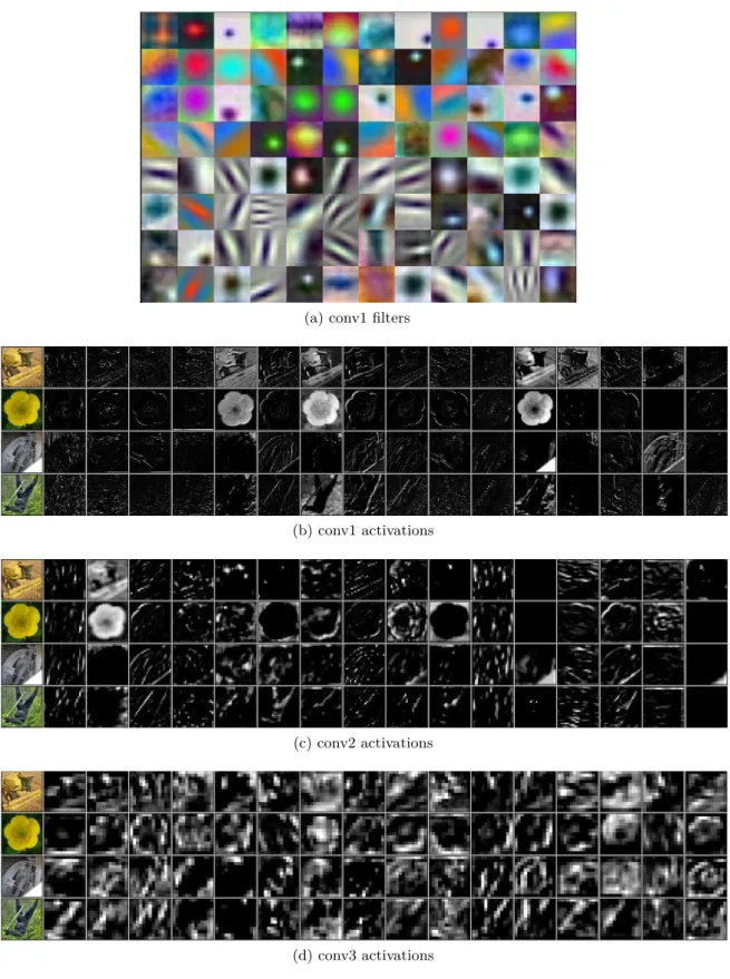
1.2 Example first layer filters and the first three layer’s outputs . . . 4

2.1 Trajectory of gradient descent in an ellipsoidal parabola . . . 15

2.2 Trajectories of SGD with different initial learning rates . . . 17

2.3 A single neuron . . . 18

2.4 Common neural network nonlinearities and their gradients . . . 20

2.5 Multi-layer perceptron . . . 21

2.6 General block form for autograd . . . 24

2.7 A convolutional layer . . . 26

2.8 Max vs Average 2×2 pooling . . . 29

2.9 LeNet-5 architecture . . . 32

2.10 The residual unit from ResNet . . . 33

2.11 Importance of phase over magnitude for images . . . 34

2.12 Typical wavelets from the 2-D separable DWT . . . 37

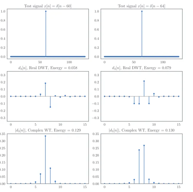
2.13 Sensitivity of DWT coefficients to zero crossings and small shifts . . . 40

2.14 Single Morlet filter with varying slants and window sizes . . . 42

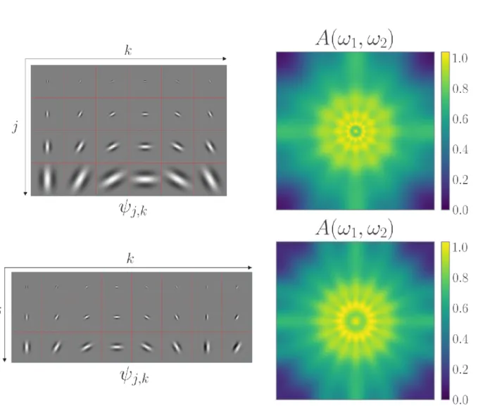
2.15 Two Morlet wavelet families and their tiling of the frequency plane . . . 43

2.16 Analysis FBs for the 1-D DTCWT . . . 45

2.17 The DWT high-high vs the DTCWT high-high frequency support . . . 47

2.18 Wavelets from the 2-D DTCWT . . . 47

2.19 A Lipschitz continuous function . . . 49

2.20 The Scattering Transform . . . 52

3.1 2-D DWT filter bank layout . . . 59

3.2 2-D DTCWT filter bank layout . . . 62

3.3 Hyperparameter results for the DTCWT ScatterNet on various datasets . . . 68

4.1 Deconvolution network block diagram . . . 75

(18)

4.3 Comparison of scattering to convolutional features . . . 81

4.4 Tiny ImageNet changes in accuracy from channel occlusion . . . 84

4.5 CIFAR changes in accuracy from channel occlusion . . . 85

4.6 Channel weights for first learned layer in a hybrid ScatterNet-CNN . . . 86

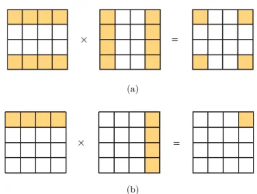
4.7 Shapes possible by filtering across the wavelet orientations with complex coefficients . . . 87

5.1 Block Diagram of Proposed Invariant Layer forj=J = 1 . . . 93

5.2 Ablation results for the invariant layer . . . 103

5.3 Ablation results for Tiny ImageNet . . . 104

6.1 Architecture using the DWT as a frontend to a CNN . . . 111

6.2 Proposed new forward pass in the wavelet domain . . . 113

6.3 Diagram of the proposed method to learn in the wavelet domain . . . 115

6.4 Forward and backward filter bank diagrams for DT_CWT gain layer . . . 116

6.5 DTCWT subbands . . . 118

6.6 Example outputs from an impulse input for the proposed gain layers . . . 120

6.7 Normalized MSE for conv layer and wavelet gain layer regression . . . 123

6.8 Large kernel ablation results for CIFAR and Tiny ImageNet . . . 126

6.9 Bandpass gain properties for network with only gain layers . . . 128

6.10 Deconvolution reconstructions for the reference architecture and purely gain layer architecture . . . 130

6.11 CIFAR-100 Ablation results with the gain layer . . . 135

7.1 Residual vs lifting layers . . . 141

7.2 Adversarial examples that can fool AlexNet . . . 142

B.1 Gradient of DWT analysis . . . 150

D.1 Filter bank diagram of 1-D DTCWT . . . 156

D.2 Filter bank diagram of 1-D DTCWT with subband gains . . . 157

F.1 Small kernel ablation results for CIFAR . . . 166

(19)

List of tables

2.1 Redundancy of scattering transform . . . 54

3.1 Hyperparameter settings for the DTCWT ScatterNet . . . 66

3.2 Comparison of properties of different ScatterNet packages . . . 69

3.3 Comparison of execution time for the forward and backward passes of the competing ScatterNet implementations . . . 69

3.4 Hybrid architectures for performance comparison . . . 71

3.5 Performance comparison for a DTCWT-based vs. a Morlet-based ScatterNet 71 5.1 Architectures for MNIST hyperparameter experiments . . . 97

5.2 Hyperparameter settings for the MNIST experiments . . . 97

5.3 Architecture performance comparison . . . 98

5.4 Modified architecture performance comparison . . . 100

5.5 CIFAR and Tiny ImageNet base architecture . . . 101

5.6 Hybrid ScatterNet models . . . 105

5.7 Hybrid ScatterNet models with convolutional layer first . . . 106

5.8 Hybrid ScatterNet top-1 classification accuracies on CIFAR . . . 107

5.9 Hybrid ScatterNet top-1 classification accuracies on Tiny ImageNet . . . 107

6.1 Ablation base architecture . . . 125

6.2 Different Nonlinearities in the Gain Layer . . . 134

A.1 Run time speeds for different layers with increasing spatial size . . . 146

(20)

(21)

Chapter 1

Introduction

It has long been the goal of computer vision researchers to be able to develop systems that can reliably recognize objects in a scene. Achieving this unlocks a huge range of applications that can benefit society as a whole: fully autonomous vehicles, automatic labelling of uploaded videos/images for searching, interpretation and screening of security video feeds, and many more, all far-reaching and extremely valuable. Many of these tasks are very tedious for humans and would be done much better by machines if the missed-detection rate can be kept low enough. The challenge does not lie in finding the right application, but in the difficulty of training a computer to see.

Some of the difficulties associated with vision are the presence of nuisance variables such as changes in lighting condition, changes in viewpoint, and background clutter. These variables do not affect the scene but can drastically change the pixel representation of it. Humans, even at early stages of their lives, have little difficulty filtering out these nuisance variables and are excellent at extracting the necessary information from a scene. To design a robust system, it makes sense to take account of how our brains see and understand scenes.

Unfortunately, biological vision is also a complex system. It has more to it than simply collecting photons in the eye. An excerpt from a recent Neurology paper [1] sums up the problem well:

It might surprise some to learn that visual information is significantly degraded as it passes from the eye to the visual cortex. Thus, of the unlimited information available from the environment, only about 1010 bits/sec are deposited in the

retina . . . only∼6×106 bits/sec leave the retina and only 114 bits/sec make it to

layer IV of V1 [2], [3]. These data clearly leave the impression that visual cortex receives an impoverished representation of the world . . . it should be noted that estimates of the bandwidth of conscious awareness itself (i.e., what we ‘see’) are in the range of 100 bits/sec or less [2], [3].

(22)

Current video cameras somewhat act as a combination of the first and second stage of this system, collecting photons in photosensitive sensors and then converting this to a stream of images. Standard definition digital television typically has a bit rate between 3×106 and

107 bits/sec (slightly larger but comparable to the 106 bits/sec travelling through the optic

nerve).

If we are to build effective vision systems, it makes sense to emulate this compression of information between the optic nerve and the later stages of the visual cortex. Hubel and Wiesel revolutionized our understanding of the (primary visual) V1 cortex in their Nobel prize-winning work (awarded in 1981 in Physiology/Medicine) by studying cats [4], [5], macaques and spider monkeys [6]. They found that neurons in the V1 cortex fired most strongly when edges of a particular (i.e., neuron-dependent) orientation were presented to the animal, so long as the edge was inside the receptive field of this neuron. Continuing on this work, Blakemore and Cooper [7] analysed the perception of kittens that had restricted visual information presented to them. In one of their experiments, the kittens were kept in darkness and then exposed for a few hours a day to only horizontal or vertical lines. After five months, they were taken into natural environments and their reactions were monitored. The two groups of cats would only play with objects when presented in an orientation that matched the orientation of their original environment. This suggests that these early layers of perception arelearned.

The current state of the art in image understanding systems are Convolutional Neural Networks (CNNs). These are a learned model that cascades many convolutional filters serially in layers, separated by nonlinearities. They are seemingly inspired by the visual cortex in the way that they are hierarchically connected, progressively compressing the information into a richer representation.

Figure 1.1 shows an example of a CNN architecture, AlexNet [8]. Inputs are resized to a manageable size, in this case, 224×224 pixels. Multiple convolutional filters of size 11×11

are convolved over this input to give 96 output channels(or activation maps). In the figure, these are split onto two graphics cards or GPUs for memory purposes. These are then passed through a pointwise nonlinear function, or nonlinearity. The activations are pooled (a form of downsampling) and convolved with more filters to give 256 new channels at the second stage. This is repeated 3 more times until the 13×13 output with 256 channels is unravelled

and passed through a fully connected neural network to classify the image as one of 1000 possible classes.

CNNs have garnered lots of attention since 2012 when AlexNet nearly halved the top-5 classification error rate (from 26% to 16%) in the ImageNet Large Scale Visual Recognition Competition (ILSVRC) [9]1. In the years since the complexity of CNNs has grown significantly.

AlexNet had only 5 convolutional layers, whereas the 2015 ILSVRC winner ResNet [15]

1

The previous state of the art classifiers had been built by combining keypoint extractors like SIFT[10] and HOG[11] with classifiers such as Support Vector Machines[12] and Fisher Vectors[13], for example [14].

(23)

1.1 Motivation | 3

Figure 1.1: Convolutional architecture example. The previous layer’s activations are combined with a learned convolutional filter. Note that while the activation maps are 3-D arrays, the convolution is only a 2-D operation. This means the filters have the same number of channels as the input and produce only one output channel. Multiple channels are made by convolving with multiple filters. Not shown here are the nonlinearities that happen in between convolution operations. Image is taken from [8].

achieved 3.57% top-5 error with 151 convolutional layers (and had some experiments with 1000 layer networks).

1.1 Motivation

Despite their success, CNNs are often criticized for beingblack-box methods. You can view the first layer of filters quite easily (see Figure 1.2a) as they exist in RGB space, but beyond that things get trickier as the filters have a third, channel dimension, typically much larger than the two spatial dimensions. Additionally, it is not clear what the input channels themselves correspond to. For illustration purposes, we have also shown some example activations from the first three convolutional layers for AlexNet inFigure 1.2(b)-(d)2. For the output from

the first convolutional layer (conv1) in Figure 1.2b, we can accurately guess that some of the filters are responding to edges or colour information, but as we go deeper to the second (conv2) and third (conv3), it becomes less and less clear what each activation is responding

to.

This has started to become a problem, and while we are happy to trust modern CNNs for isolated tasks, we are less likely to be comfortable with them driving cars through crowded cities, or making executive decisions that affect people directly. In a commonly used contrived example, it is not hard to imagine a deep network that could be used to assess whether giving a bank loan to an applicant is a safe investment. Trusting a black box solution is deeply unsatisfactory in this situation. Not only from the customer’s perspective, who, if declined,

2

These activations are taken after a specific nonlinearity that sets negative values to 0, hence the large black regions.

(24)

(a) conv1 filters

(b) conv1 activations

(c) conv2 activations

(d) conv3 activations

Figure 1.2: Example first layer filters and the first three layer’s outputs. (a) The 11×11 filters for the first stage of AlexNet. Of the 96 filters, 48 were learned on one GPU and

another 48 on another GPU. Interestingly, one GPU has learned mostly lowpass/colour filters and the other has learned oriented bandpass filters. (b) - (d)Randomly chosen activations from the output of the first, second and third convolutional layers of AlexNet (seeFigure 1.1) with negative values set to 0. Filters and activation images are taken from the supplementary material of [8].

(25)

1.2 Approach | 5 has the right to know why [16], but also from the bank’s — before lending large sums of money, most banks would like to know why the network has given the ‘all clear’. ‘It has worked well before’ is a poor rule to live by.

Aside from their lack of interpretability, it often takes a long time and a lot of effort to train state-of-the-art CNNs. Typical networks that have won ILSVRC since 2012 have had roughly 100 million parameters and take up to a week to train. This is optimistic and assumes that you already know the necessary optimization or architecture hyperparameters, which you often have to find out by trial and error. In a conversation we had with Yann LeCun, the attributed father of CNNs, at a Computer Vision Summer School (ICVSS 2016), LeCun highlighted this problem himself:

“There are certain recipes (for building CNNs) that work and certain recipes that don’t, and we don’t know why.”

Considering the recent success of CNNs, it is becoming more and more important to understand how and what a network learns, so we can interrogate what in the input has contributed to it making its classification or regression choice. Without this information, the use of these incredibly powerful tools could be restricted to research and proprietary applications.

1.2 Approach

The structure of convolutional layers is fairly crude in terms of signal processing - arbitrary taps of an FIR filter are learned typically via stochastic gradient descent from random starting states to minimize either a mean-squared error or cross-entropy loss.

This leads us to ask a motivating question:

Is it possible to learn convolutional filters as combinations of basis functions rather than individual filter taps?

In achieving this, it is important to find ways to have an adequate richness of filtering while reducing the number of parameters needed to specify resulting filters. We want to contract the space of learning to a subspace or manifold that is more useful. In much the same way, the convolutional layer in a CNN is a restricted version of a fully connected layer in a multi-layer perceptron, yet adding this restriction allowed us to train more powerful networks.

The intuition that we explore in this thesis is thatcomplex wavelets are good basis functions for filtering in CNNs.

(26)

1.2.1 Why Complex Wavelets?

Most modern approaches to CNNs are framed entirely in the spatial domain; our choice of complex wavelets as the basis function to explore comes from the deeper intuition that it may be helpful to rethink about CNNs in the frequency domain. Historically, the frequency domain has been an excellent space for solving many signal processing problems such as noise removal, filter design, edge detection and data compression. We believe it may prove to have advantages for CNNs too (beyond just an efficient space to do convolution in).

The Fourier transform, which uses complex sinusoids as its basis function, is perhaps the most ubiquitous tool to use for frequency domain analysis. The problem with these complex sinusoids is that they have infinitesupport. This means that small changes in one part of an image affect every Fourier coefficient. Additionally, they are not stable to small deformations, as small changes can produce unbounded changes in the representation [17].

The common remedy to this problem is to use the localized, and more stable, short-time Fourier transform (STFT). The STFT (or the Gabor transform) is a natural extension of the Fourier transform, windowing the complex sinusoids with a Gaussian (or similar) function. The STFT has the undesirable property that all frequencies are sampled with the same resolution. A close relative of the STFT is the continuous wavelet transform (CWT). The shorter duration of the wavelet basis functions as the frequency increases means that their time resolving power improves with centre-frequency. Another commonly used wavelet transform is the discrete wavelet transform (or the DWT) often favoured over the CWT because of its speed of computation. It can use many different finite support basis functions, all with different frequency localization properties, but it is usually limited to using real filters. As such, it suffers from many problems such as shift-dependence and lack of directionality in two dimensions (2-D). These problems can be remedied by using the slower CWT with complex basis functions, but we choose instead to use the dual-tree complex wavelet transform, or DTCWT [18] with q-shift filters [19].

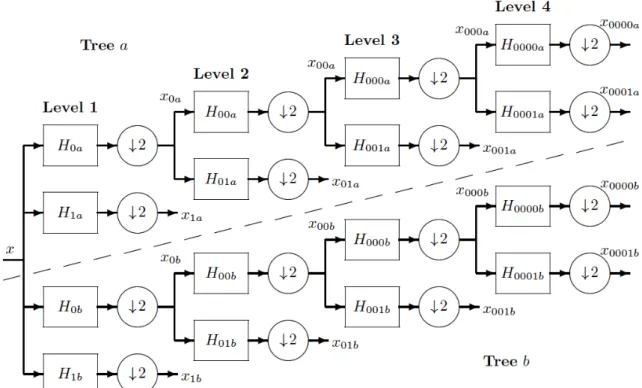
The DTCWT allows for complex basis functions that have shift-invariance and direc-tionality, while being fast to implement like the DWT (in 2-D it can be thought of as the application of 4 DWTs in parallel). It is also more easily invertible than the CWT, forming a tight frame [20], which we believe may prove to be a very important property for visualizing what a CNN is responding to.

We revisit the properties of the Fourier transform, STFT, CWT, DWT and DTCWT and expand on the properties behind our choice of basis functions in the literature review

section 2.6.

On top of the intuition that the wavelet domain is a good space in which to frame CNNs, there are some experimental motivating factors too. Firstly, the wavelet transform has had much success in image and video compression, particularly for JPEG2000 [21]. Good compression performance implies an ability of the basis functions to represent the input

(27)

1.3 Method | 7 data sparsely (as seems to happen in the brain). Secondly, the filters from the first layer of AlexNet (Figure 1.2) look like oriented wavelets. Given that there was no prior placed on the filters to make them have this similarity to wavelets, this result is noteworthy. And finally, the aforementioned work of Hubel and Wiesel suggests that the early layers of the visual system act like a Gabor transform.

These experimental observations imply that complex wavelets would do well in replacing the first layer of a CNN, but we would also like to find out if they can be used at deeper layers. Their well-understood and well-defined behaviour would help us to answer the above how andwhy questions. Additionally, they allow us to enforce a certain amount of smoothness and near orthogonality; smoothness seems to be important to avoid sensitivity to adversarial or spoofing attacks [22] and near orthogonality allows you to cover a large space with fewer coefficients.

But first, we must find outif it is possible to get the same or nearly the same performance by using wavelets as the building blocks for CNNs, and this is the core goal of this thesis.

1.3 Method

1.3.1 ScatterNets

To explore the uses of complex wavelets in CNNs, we begin by looking at one of the most popular current uses of wavelets in image recognition tasks, the Scattering Transform.

The Scattering Transform, or theScatterNet, was introduced in [17], [23] at the same time as AlexNet. It is a non-black-box network that can be thought of as a restricted complex-valued CNN [24]. Unlike a CNN, it has predefined convolutional kernels, set to complex wavelet (and scaling) functions and uses the complex magnitude as its nonlinearity. Due to its well-defined structure, it can be analyzed and bounds on its stability to shifts, noise and deformations are found in [17].

For a simple task like identifying small handwritten digits, the variabilities in the data are simple and small and the ScatterNet can reduce the problem into a space which a Gaussian Support Vector Machine (or SVM [12]) can easily solve [23]. For a more complex task like identifying real-world objects, the ScatterNet can somewhat reduce the variabilities and get good results with an SVM, but there is a significant performance gap between this and what a CNN can achieve. For example, in [25] a second-order ScatterNet can achieve 82.3% top-1

classification accuracy on CIFAR-10, a commonly used dataset, whereas modern CNNs such as [15] can achieve 93.4%.

1.3.2 Learnable ScatterNets

To start to address the performance gap between ScatterNet front ends and CNNs we first investigate the properties of current ScatterNets. Inspired by the visualization work of

(28)

Zeiler and Fergus [26] we build a DeScatterNet. The DeScatterNet leverages the perfect reconstruction properties of the DTCWT and allows us to investigate what in the input image the ScatterNet is responding to.

Interpretring the visualizations from the DeScatterNet leads us to the conclusion that the ScatterNet may be limiting itself by not combining the filtering of different wavelet orientations (it does not mix the channels as a CNN does). Inspired by the work of [27], we propose the learnable ScatterNet, which includes this mixing, while keeping the desirable properties of the ScatterNet (invariance to translation, additive noise, and deformations; see

subsection 2.7.1for a description of these properties).

The learnable ScatterNet can be thought of as using the scattering outputs as the basis functions3for our convolutional layers. We show that this improves greatly on the ScatterNet design, and under certain constraints can improve on the performance of CNNs too.

1.3.3 Wavelet Domain Filtering

We find that the complex modulus of the ScatterNet design to be useful for some operations in a CNN, but it has a demodulating effect on the frequency energy (all the outputs have significantly more energy in lower frequencies). This limits repeated application of it as the demodulating effect compounds.

We develop a system that does not use the complex modulus; instead, it learnscomplex gains in the wavelet domain. Rather than mixing subbands together, we keep them indepen-dent and only learn to mix across the channel dimension. This is important, as it allows us to then use the inverse DTCWT to return to the pixel domain. The shift-invariant properties of the DT_CWT mean the reconstructed outputs are (mostly) free from aliasing effects, despite much of the processing being carried out at significantly reduced sample rates in the wavelet domain.

We show that our layer can be used alongside regular convolutional layers. I.e., it becomes possible to ‘step’ into the wavelet domain to do wavelet filtering for one layer, before ‘stepping’ back into the pixel domain to do pixel filtering for the next layer.

1.4 Thesis Layout and Contributions to Knowledge

This thesis has one literature review chapter and four novel-work chapters:

• Chapter 2 explores some of the background necessary for starting to develop image understanding models. In particular, it covers the inspiration for CNNs and the workings of CNNs themselves, as well as covering the basics of wavelets and ScatterNets.

3

Although they are not true basis functions as they are the combination of a complex wavelet with a modulus nonlinearity, and are thus data-dependent.

(29)

1.4 Thesis Layout and Contributions to Knowledge | 9 • Chapter 3proposes a change to the core of the ScatterNet. In addition to performance issues with ScatterNets, they are slow and both memory-intensive and compute-intensive to calculate. This in itself is enough of an issue to make it unlikely that they would be used as part of deep networks. To overcome this, we change the computation to use the DT_CWT [18] instead of Morlet wavelets, achieving a 20 to 30 times speed-up while achieving a small improvement in classification performance.

• Chapter 4 describes our DeScatterNet, a tool used to interrogate the structure of ScatterNets. We also perform tests to determine the usefulness of the different scattered outputs finding that many of them are not useful for image classification.

• Chapter 5describes the Learnable ScatterNet we have developed to address some of the issues found from the interrogation in chapter 4. We find that a learnable ScatterNet layer performs better than a regular ScatterNet, and can improve on the performance of a CNN if used instead of pooling layers. We also find that scattering works well not just on RGB images, but can also be useful when used after one layer of learning. • Inchapter 6, we step away from ScatterNets and present the Wavelet Gain Layer. The

gain layer uses the wavelet space as a latent space to learn representations. We find possible nonlinearities and describe how to learn in both the pixel and wavelet domain. This work showed that there may well be benefits to learning in the wavelet domain for earlier layers of CNNs, but we have not yet found advantages to using the wavelet gain layer for deeper layers.

1.4.1 Contributions and Publications The key contributions of this thesis are:

• Software for wavelets and DT_CWT based ScatterNet (described in chapter 3) and publicly available at [28].

• ScatterNet analysis and visualizations (described in chapter 4). This chapter expands on the paper we presented at MLSP2017 [29].

• Invariant Layer/Learnable ScatterNet (described inchapter 5)). This chapter expands on the paper accepted at ICIP2019 [30]. Software available at [31].

• Learning convolutions in the wavelet domain (described inchapter 6). We have published preliminary results on this work to arXiv [32] but have expanded on this paper in the chapter. Software available at [33].

(30)

1.4.2 Related Research

Readers may also be interested in the theses [34] and [35].

In [34] Singh looks at using the ScatterNet as a fixed front end and combining it with well-known machine learning methods such as SVMs, Autoencoders and Restricted Boltzmann Machines. By combining frameworks in a defined way he creates unsupervised feature extractors which can then be used with simple classifiers. Some relevant papers that make up this thesis are [36]–[38]. In [36] Singh shows that the DTCWT-ScatterNet outperforms a Morlet-ScatterNet when used as a front end for an SVM, which is similar to the work we do in chapter 3where we show the DTCWT-ScatterNet outperforms a Morlet-ScatterNet when used as a front end for CNNs. He then expands on this work by testing other backends in [37], [38].

In [35] Oyallon looks at ScatterNets as front ends to deeper learning systems, such as CNNs. Some relevant papers that make up Oyallon’s thesis are [25], [39]. [39] is particularly relevant as he uses a ScatterNet as a feature extractor for a CNN. We do similar research in

(31)

Chapter 2

Background

2.1 Chapter Layout

This thesis combines work in several fields. We provide a background for the most important and relevant fields in this chapter. We first introduce the basics of deep learning, looking at general supervised learning in section 2.2 before more specifically examining the structure of Neural Networks insection 2.3and CNNs in section 2.4.

We then define the properties of Wavelet Transforms, looking at the difference between the discrete WT and the complex Morlet and DT_CWT insection 2.6. Finally, we introduce the Scattering Transform or ScatterNet, the original inspiration for this thesis in section 2.7.

2.2 Supervised Machine Learning

While this subject is general and covered in many places, we take inspiration from [40] (chapters 1, 2, 7, 8) and [41] (chapter 5-10). Consider a sample space over inputs and targets X×_Y and a data generating distribution pdata. Given a dataset of input-target

pairsD={(x(n)_{, y}(n))_}N

n=1 we would like to make predictions aboutpdata(y|x) that generalize

well to unseen data. A common way to do this is to build a parametric model to directly estimate this conditional probability. For example, regression asserts the data are distributed according to a function of the inputs plus a noise term ϵ:

y=f(x, θ) +ϵ (2.2.1)

This noise is often modelled as a zero-mean Gaussian random variable,ϵ∼_N(0, σ2_I), which

means we can write:

pmodel(y|x, θ, σ2) =_N(_y; _f(_{x, θ})_{, σ}2_I) (2.2.2)

(32)

We can find point estimates of the parameters by maximizing the likelihood ofpmodel(y|x, θ)

(or equivalently, minimizing KL(pmodel||pdata), the KL-divergence betweenpmodel andpdata). As the data are all assumed to be i.i.d., we can multiply individual likelihoods, and solve for

θ: θM LE= argmax θ pmodel(y|x, θ) (2.2.3) = argmax θ N Y n=1 pmodel(y(n)|x(n), θ) (2.2.4) = argmax θ N X n=1 logpmodel(y(n)_|_x(n)_{, θ}₎ _(2.2.5)

Using the Gaussian regression model from above, this becomes:

θM LE= argmax θ N X n=1 logpmodel(y(n)|x(n), θ) (2.2.6) = argmax θ −Nlogσ−N 2 log(2π)− N X n=1 y(n)₋_f(_x(n)_{, θ})2 2σ2 ! (2.2.7) = argmin θ 1 N N X n=1 y(n)₋_f(_x(n)_{, θ})2 2 (2.2.8)

which gives us the well-known result that we would like to find parameters that minimize the mean squared error (MSE) between targets y and predictions ˆy=f(x, θ).

For binary classification y∈ {0,1} and instead of the model in (2.2.2), we have:

pmodel(y|x, θ) = Ber(y; σ(f(x, θ))) (2.2.9)

whereσ(x) is the sigmoid function and Ber is the Bernoulli distribution. Note that we have

used σ to refer to noise standard deviation thus far but now useσ(x) to refer to the sigmoid

and softmax functions, a confusing but common practice. σ(x) and Ber(y;p) are defined as: σ(z) = 1

1 +e−z (2.2.10)

Ber(y;p) =pI(y=1)(1−p)I(y=0) (2.2.11)

where I(x) is the indicator function. The sigmoid function is useful here as it can convert a

real outputf(x, θ) into a probability estimate. In particular, large positive values get mapped

to 1, large negative values to 0, and values near 0 get mapped to 0.5 [41, Chapter 6]. This expands naturally to multi-class classification by makingy a 1-hot vector in {0,1}C. We must also swap the Bernoulli distribution for the Multinoulli or Categorical distribution,

(33)

2.2 Supervised Machine Learning | 13 and the sigmoid function for a softmax. The softmax function for vector z is defined as:

σi(z) = e

zi

PC

k=1ezk

(2.2.12) which has the nice properties that 0≤σi≤1 and Piσi= 1. The categorical distribution uses the softmax output:

Cat(y;σ) = C Y c=1 σI(yc=1) c (2.2.13)

If we let ˆyc=σc(f(x, θ)), this makes (2.2.9):

pmodel(y|x, θ) = Cat(y; σ(f(x, θ))) (2.2.14) =YC c=1 N Y n=1 ˆ y_c(n)I(y (n) c =1) (2.2.15) As y(cn) is either 0 or 1, we remove the indicator function. Maximizing this likelihood to find the ML estimate for θ:

θM LE= argmax θ C Y c=1 N Y n=1 ˆ y_c(n)y (n) c (2.2.16) = argmax θ 1 N N X n=1 C X c=1 y_c(n)log ˆy_c(n) (2.2.17)

which we recognize as the cross-entropy betweeny and ˆy.

2.2.1 Priors on Parameters and Regularization

Maximum likelihood estimates for parameters, while straightforward, can often lead to overfitting. A common practice is to regularize learnt parameters θby putting a prior over

them. If we do not have any prior information about what we expect them to be, it may still be useful to put an uninformative prior over them. For example, if our parameters are in the reals, a commonly used uninformative prior is a Gaussian.

Let us extend the regression example from above by saying we would like the prior on the parametersθ to be a Gaussian, i.e. p(θ) =_N(0, τ2_I

(34)

posteriori (MAP) estimate is then obtained by finding: θM AP = argmax θ p(θ|_D, σ2) (2.2.18) = argmax θ p(y|x, θ, σ2)_p(_θ) p(y|x) (2.2.19) = argmax θ logp(y|x, θ, σ2) + log_p(_θ) (2.2.20) = argmin θ 1 N N X n=1 y(n)₋_f(_x(n)_{, θ})2 2 + λ 2||θ||22 (2.2.21)

whereλ=σ2_/τ2is the ratio of the observation noise to the strength of the prior [40, Chapter 7].

This is equivalent to minimizing the MSE with an ℓ2 penalty on the parameters, also known

as ridge regression or penalized least squares. λis often called weight decay in the neural network literature, which we will also use in this thesis.

2.2.2 Loss Functions and Minimizing the Objective

It may be useful to rewrite (2.2.18) as an objective function on the parameters J(θ): J(θ) = 1 N N X n=1 y(n)₋_f(_x(n)_{, θ})2 2 + λ 2||θ||22 (2.2.22) =Ldata(y, f(x, θ)) +Lreg(θ) (2.2.23)

whereLdatais the data loss such as MSE or cross-entropy andLreg is the regularization, such asℓ2 orℓ1 penalized loss. NowθM AP = argminθJ(θ).

Finding the global minimum of the objective function is task-dependent and is often not straightforward. One commonly used technique is called gradient descent (GD). This is not difficult to do as it only involves calculating the gradient at a given point and taking a small step in the direction of steepest descent. The update equation for GD is:

θt+1=θt−η

∂J

∂θ (2.2.24)

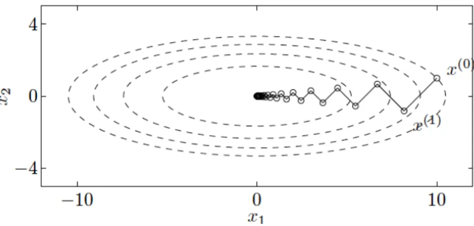
Unsurprisingly, such a simple technique has limitations. In particular, it is sensitive to the choice of step size and has a slow convergence rate when the condition number (ratio of largest to smallest eigenvalues) of the Hessian around the optimal point is large [42]. An example of this is shown inFigure 2.1. In this figure, the step size is chosen with exact line search, i.e. η= argmin s f x+s∂f ∂x (2.2.25)

(35)

2.2 Supervised Machine Learning | 15

Figure 2.1: Trajectory of gradient descent in an ellipsoidal parabola. Some contour lines of the function f(x) = 1/2 x2

1+ 10x22

and the trajectory of GD optimization using exact line search. This space has condition number 10, and shows the slow convergence of GD in spaces with largely different eigenvalues. Image is taken from [42] Figure 9.2.

To truly overcome this problem, we must know the curvature of the objective function ∂2_J

∂θ2. An example optimization technique that uses the second-order information is Newton’s

method [42, Chapter 9]. Such techniques sadly do not scale with size, as computing the Hessian is proportional to the number of parameters squared, and many neural networks have hundreds of thousands, if not millions of parameters. In this thesis, we only consider first-order optimization algorithms.

2.2.3 Stochastic Gradient Descent

Aside from the problems associated with the curvature of the functionJ(θ), another common

issue faced with the gradient descent of (2.2.24) is the cost of computing ∂J

∂θ. In particular, the first term:

Ldata(y, f(x, θ)) =Ex,y∼pdata[Ldata(y, f(x, θ))] (2.2.26)

= 1 N N X n=1 Ldata y(n), f(x(n), θ) (2.2.27)

involves evaluating the entire dataset at the current values of θ. As the training set size

grows into the thousands or millions of examples, this approach becomes prohibitively slow. Equation (2.2.26) writes the data loss as an expectation, hinting at the fact that we can remedy this problem by using fewer samples Nb< N to evaluate Ldata. This variation is called Stochastic Gradient Descent (SGD).

Choosing the batch size is a hyperparameter choice that we must think carefully about. Setting the value very low, e.g. Nb= 1 can be advantageous as the noisy estimates for the gradient have a regularizing effect on the network [43]. Increasing the batch size to larger

(36)

values allows you to easily parallelize computation as well as increasing accuracy for the gradient, allowing you to take larger step sizes [44]. A good initial starting point is to set the batch size to 128 samples and increase/decrease from there [41].

2.2.4 Gradient Descent and Learning Rate

The step size parameter,η in (2.2.24) is commonly referred to as the learning rate. Choosing

the right value for the learning rate is key. Unfortunately, the line search algorithm in (2.2.25) would be too expensive to compute for neural networks (as it would involve evaluating the function several times at different values), each of which takes about as long as calculating the gradients themselves. Additionally, as the gradients are typically estimated over a mini-batch and are hence noisy there may be little added benefit in optimizing the step sizes in the estimated direction.

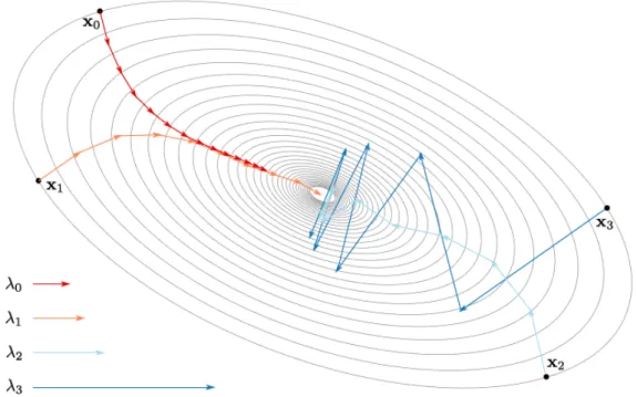
Figure 2.2illustrates the effect the learning rate can have over a contrived convex example. Optimizing over more complex loss surfaces only exacerbates the problem. Sadly, choosing the initial learning rate is ‘more of an art than a science’ [41], but [45], [46] have some tips on what to how to set it. We have found in our work that searching for a large learning rate that causes the network to diverge and reducing it from there can be a good search strategy. This agrees with Section 1.5 of [47] which states that for regions of the loss space which are roughly quadratic,ηmax= 2ηopt and any learning rate above 2ηopt causes divergence.

On top of the initial learning rate, the convergence of SGD methods require [45]: ∞ X t=1 ηt→ ∞ (2.2.28) ∞ X t=1 η2 t <∞ (2.2.29)

Choosing how to do this also contains a good amount of artistry, and there is no one scheme that works best. A commonly used greedy method is to keep the learning rate constant until the training loss stabilizes and then to enter the next phase of training by settingηk+1=γηk where γ is a decay factor. Settingγ and the thresholds for triggering a step however must be

chosen by monitoring the training loss curve and trial and error [45].

2.2.5 Momentum and Adam

One simple and very popular modification to SGD is to add momentum. Momentum accumulates past gradients with an exponential-decay moving average and continues to move in their direction. The name comes from the comparison of finding minima to rolling a ball over a surface – any new force (newly computed gradients) must overcome the current momentum of the ball. This has a smoothing effect on noisy gradients.

(37)

2.2 Supervised Machine Learning | 17

Figure 2.2: Trajectories of SGD with different initial learning rates. This figure illustrates the effect the step size has over the optimization process by showing the trajectory forη=λi from equivalent starting points on a symmetric loss surface. Increasing the step size beyond λ3 can cause the optimization procedure to diverge. Image taken from [48] Figure

2.7.

We can achieve momentum by creating avelocity variablevt and modify (2.2.24) to be:

vt+1=αvt−ηk

∂J

∂θ (2.2.30)

θt+1=θt+vt+1 (2.2.31)

where 0≤α <1 is the momentum term indicating how quickly to ‘forget’ past gradients.

Another popular modification to SGD is the adaptive learning rate technique Adam [49]. There are several other adaptive schemes such as AdaGrad [50] and AdaDelta [51], but they are all quite similar, and Adam is often considered the most robust of the three [41]. The goal of all of these adaptive schemes is to take larger update steps in directions of low variance, helping to minimize the effect of large condition numbers we saw in Figure 2.1. Adam does this by keeping track of the firstmt and secondvt moments of the gradients:

gt+1= ∂J

∂θ (2.2.32)

mt+1=β1mt+ (1−β1)gt+1 (2.2.33) vt+1=β2vt+ (1−β2)g2t+1 (2.2.34)

(38)

x1 Input 1 x2 Input 2 x3 Input 3 x4 Input 4 x5 Input 5 1 y Output w1 w2 w3 w4 w5 b

Figure 2.3: A single neuron. The neuron is composed of inputs xi, weights wi (and a bias term), as well as an activation function. Typical activation functions include the sigmoid function, tanh function and the ReLU

where 0≤β1, β2<1. Note the similarity between updating the mean estimate in (2.2.33)

and the velocity term in (2.2.30)1. The parameters are then updated with: θt+1=θt−η

mt+1 √

vt+1+ϵ

(2.2.35) where ϵis a small value to avoid dividing by zero.

2.3 Neural Networks

2.3.1 The Neuron and Single-Layer Neural Networks

The neuron, shown in Figure 2.3is the core building block of neural networks. It takes the dot product between an input vectorx∈RD and a weight vector_w, before applying a chosen nonlinearity. Historically, the sigmoid nonlinearity was the most popular but today other functions have become more popular. Still, the convention has remained to name this generic nonlinearity σ. I.e. y=σ(⟨x,w⟩) =σ D X i=0 xiwi ! (2.3.1) where we have used the shorthandb=w0 andx0= 1. Also, note that we will use the common

practice in the neural network literature to call the parametersweights denoted byw. 1

Themt+1andvt+1 terms are then bias-corrected as they are biased towards zero at the beginning of

(39)

2.3 Neural Networks | 19 Some of the other popular nonlinear functionsσ are the tanh and ReLU:

tanh(x) =e

x₋_e−x

ex+_e−x (2.3.2)

ReLU(x) = max(x,0) (2.3.3)

See Figure 2.4 for plots of these. The original Rosenblatt perceptron [52] also used the Heaviside function H(x) =I(x >0).

Note that if⟨w,w⟩= 1 then ⟨x,w⟩ is the distance from the point xto the hyperplane with normalw(with non-unit-normw, this can be thought of as a scaled distance). Thus, the weight vector wdefines a hyperplane in RD which splits the space into two. The choice of nonlinearity then affects how points on each side of the plane are treated. For a sigmoid, points far below the plane get mapped to 0 and points far above the plane get mapped to 1 (with points near the plane having a value of 0.5). For tanh nonlinearities, these points get mapped to -1 and 1. For ReLU nonlinearities, every point below the plane (⟨x,w⟩<0) gets

mapped to zero and every point above the plane keeps its inner product value.

Nearly all modern neural networks use the ReLU nonlinearity and it has been credited with being a key reason for the recent surge in deep learning success [53], [54]. In particular: 1. It is less sensitive to initial conditions as the gradients that backpropagate through it will be large even ifxis large. A common observation of sigmoid and tanh nonlinearities

was that their learning would be slow for quite some time until the neurons came out of saturation, and then their accuracy would increase rapidly before levelling out again at a minimum [55]. The ReLU, on the other hand, has a constant gradient when it is activated.

2. It promotes sparsity in outputs, by setting them to a hard 0. Studies on brain energy expenditure suggest that neurons encode information in a sparse manner. [56] estimates the percentage of neurons active at the same time to be between 1 and 4%. Sigmoid and tanh functions will typically have all neurons firing, while the ReLU can allow neurons to fully turn off.

2.3.2 Multilayer Perceptrons

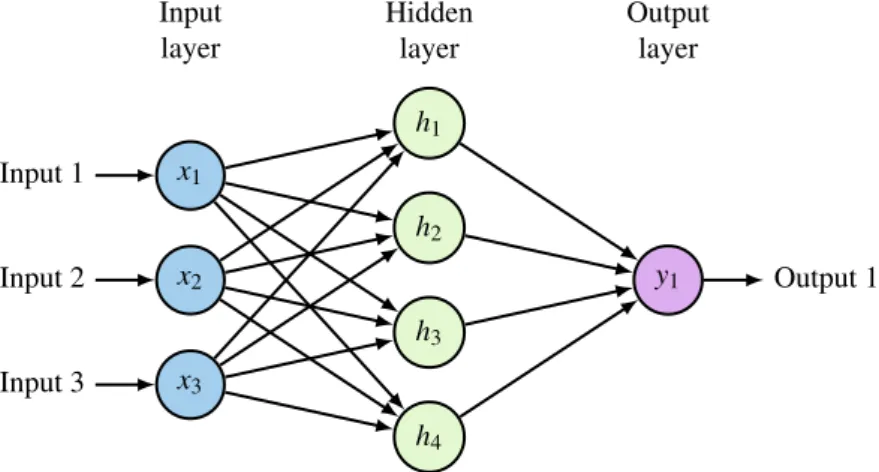
As mentioned in the previous section, a single neuron can be thought of as a separating hyperplane with an activation that maps the two halves of the space to different values. Such a linear separator is limited and famously cannot solve the XOR problem [57]. Fortunately, adding a single hidden layer like the one shown in Figure 2.5 can change this, and it is proveable that with an infinitely wide hidden layer, a neural network can approximate any function [58], [59]. This extension is called a multilayer perceptron, or MLP.

(40)

x y −2 −1 1 2 −1 1 2 y=σ(x) y=tanhx y=ReLU(x) y −2 −1 1 2 −1 2 1 y=σ0(x) y=tanh0(x) y=ReLU0₍_x₎

Figure 2.4: Common neural network nonlinearities and their gradients. The sigmoid, tanh and ReLU nonlinearities are commonly used activation functions for neurons. The tanh and sigmoid have the nice property of being smooth but can have saturation when the input is either largely positive or largely negative, causing little gradient to flow back through it. The ReLU does not suffer from this problem and has the additional nice property of setting values to exactly 0, making a sparser output activation.

The forward pass of such a network with one hidden layer ofH units is: hi=σ   D X j=0 xjw(1)ij   (2.3.4) y= H X k=0 hkw(2)k (2.3.5)

wherew(l) denotes the weights for the_l-th layer, of which Figure 2.5has 2. Note that these

individual layers are often called fully connected as each node in the previous layer affects every node in the next.

If we were to expand this network to haveNlsuch fully connected layers, we could rewrite the action of each layer in a recursive fashion:

y(l+1)=W(l+1)x(l) (2.3.6)

x(l+1)=σy(l+1) (2.3.7)

where W is now a weight matrix, acting on the vector of the previous layer’s outputsx(l).

As we are now considering every layer to be an input to the next stage, we have removed the

h notation and added the superscript (l) to define the depth. x(0) is the network input and y(Nl) is the network output. Let us say that the output has_C nodes, and a hidden layer _x(l)

hasCl nodes.

2.3.3 Backpropagation

It is important to truly understand backpropagation when designing neural networks, so we describe the core concepts now for a neural network with Nl layers.

(41)

2.3 Neural Networks | 21 x1 Input 1 x2 Input 2 x3 Input 3 h1 h2 h3 h4 y1 Output 1 Hidden layer Input

layer Outputlayer

Figure 2.5: Multi-layer perceptron. Expanding the single neuron from Figure 2.3 to a network of neurons. The internal representation units are often referred to as the hidden layer as they are an intermediary between the input and output.

The delta rule, initially designed for networks with no hidden layers [60], was expanded to what we now considerbackpropagation in [61]. While backpropagation is conceptually just the application of the chain rule, Rumelhart, Hinton, and Williams successfully updated the delta rule to networks with hidden layers, laying a key foundational step for deeper networks.

With a deep network, calculating ∂Ldata

∂w may not seem easy, particularly if w is a weight in one of the earlier layers. We need to define a rule for updating the weights in all Nl layers of the network, W(1)_{, W}(2)_{, . . . W}(Nl) however, only the final set_W(Nl) are connected to the

data loss function Ldata.

2.3.3.1 Regression Loss

Let us start with writing down the derivative of L (dropping the data subscript for now) with respect to the network output ˆy=y(Nl) using the regression objective function (2.2.8).

∂L ∂y(Nl) = ∂ ∂yˆ 1 N Nb X n=1 1 2 y(n)−yˆ(n)2 ! (2.3.8) = 1 N Nb X n=1 ˆ y(n)−y(n) (2.3.9) =e∈R (2.3.10)

where we have used the fact that for the regression case,y(n)_, _yˆ(n)_∈_R.

2.3.3.2 Classification Loss

For the classification case (2.2.17), let us keep the output of the network as y(Nl)_∈RC and

define ˆy as the softmax applied to this vector ˆyc(n)=σc y(Nl,n)

(42)

Note that the softmax is a vector-valued function going fromRC_→_RC so has a Jacobian matrixS with values:

Sij = ∂yˆi ∂y(Nl) j =    σi(1−σj) ifi=j −σiσj ifi̸=j (2.3.11) Now, let us return to (2.2.17) and find the derivative of the objective function to this output value ˆy: ∂L ∂yˆ = ∂ ∂yˆ 1 N Nb X n=1 C X c=1 y_c(n)log ˆy_c(n) ! (2.3.12) = 1 N Nb X n=1 C X c=1 yc(n) ˆ yc(n) (2.3.13) =d∈RC (2.3.14)

Note that unlike (2.3.10), this derivative is vector-valued. To find ∂L

∂y(Nl) we use the chain rule. It is easier to find the partial derivative with respect to one node in the output first, and then expand from here, i.e.:

∂L ∂y(Nl) j =XC i=1 ∂L ∂yˆi ∂yˆi ∂y(Nl) j (2.3.15) =ST j d (2.3.16)

where Sj is the jth column of the Jacobian matrix S. It becomes clear now that to get the entire vector derivative for all nodes iny(Nl), we must multiply the transpose of the Jacobian

matrix with the error term from (2.3.14):

∂L ∂y(Nl) =S

T_d _(2.3.17)

2.3.3.3 Final Layer Weight Gradient

Let the final weight layer be calledW ∈RC×CNl−1 (where _C

Nl−1 is the number of outputs at

the penultimate layer). We call the gradient for the final layer weights the update gradient. It can be computed by the chain rule again. For an individual entry in this matrix Wij, the update gradient is:

∂J ∂Wij = ∂Ldata ∂yi ∂yi ∂Wij + λWij (2.3.18) =∂Ldata ∂yi xj+λWij (2.3.19)

(43)

2.3 Neural Networks | 23 where the second term in the above two equations comes from the regularization loss that is added to the objective. The update gradient of the entire weight matrix is then:

∂J ∂W(Nl) = ∂Ldata ∂yˆ x T_{+ 2}_λW _(2.3.20) =STdx(Nl−1) T + 2λW(Nl)_∈RC×C_Nl−1 (2.3.21)

2.3.3.4 Final Layer Passthrough Gradient

We also want to find the passthrough gradients of the final layer ∂L

∂x(_Nl−1) (these are not

affected by the regularization terms, so we only need to find the gradient w.r.t. the data loss

L). In a similar fashion, we first find the gradient with respect to individual elements in x(Nl−1) before generalizing to the entire vector:

∂L ∂xi = C X j=1 ∂L ∂yj ∂yj ∂xi (2.3.22) = C X j=1 ∂L ∂yj Wj,i (2.3.23) =W_iT∂L ∂y (2.3.24) (2.3.25) whereWi is the ith column of W. Thus

∂L ∂x(Nl−1) = W(Nl) T _∂L ∂y(Nl) (2.3.26) =W(Nl) T STd (2.3.27)

This passthrough gradient then can be used to update the next layer’s weights by repeating

subsubsection 2.3.3.3 and subsubsection 2.3.3.4. 2.3.3.5 General Layer Update

The easiest way to handle this flow of gradients and the basis for most automatic differentiation packages is the block definition shown inFigure 2.6. For all neural network components (even if they do not have weights), the operation must not only be able to calculate the forward passy=f(x, w) given weights w and inputsx, but also calculate theupdate andpassthrough gradients ∂L

∂w, ∂L

∂x given an input gradient ∂L

∂y. The input gradient will have the same shape as y as will the update and passthrough gradients match the shape ofw andx. This way,

gradients for the entire network can be computed in an iterative fashion starting at the loss function and moving backwards.

(44)

y =f(x, w) x ∂L ∂x w ∂L ∂w y ∂L∂y

Figure 2.6: General block form for autograd. All neural network functions need to be able to calculate the forward passy=f(x, w) as well as the update and passthrough gradients

∂L ∂w,

∂L

∂x. Backpropagation is then easily done by allowing data to flow backwards through these blocks from the loss.

2.4 Convolutional Neural Networks

Convolutional Neural Networks (CNNs) are a special type of Neural Network built mainly from convolutional layers rather than fully connected layers. A convolutional layer is one where the weights are shared spatially across the layer. In this way, a neuron at is only affected by nodes from the previous layer in a given neighbourhood, rather than from every node.

First popularized in 1998 by LeCun et. al. in [62], the convolutional layer was introduced to build invariance with respect to translations, as well as reduce the parameter size of early neural networks for pattern recognition. The idea of having a locally-receptive field had already been shown to be a naturally occurring phenomenon by Hubel and Wiesel [5]. They did not become popular immediately, and another spatially based keypoint extractor, SIFT [10], was the mainstay of detection systems until the AlexNet CNN [8] won the 2012 ImageNet challenge [63] by a large margin over the next competitors, many of whom used SIFT. This CNN had 5 convolutional layers followed by 3 fully connected layers.

We now briefly describe the convolutional layer, as well as many other layers used in CNNs that have become popular in the past few years.

2.4.1 Convolutional Layers

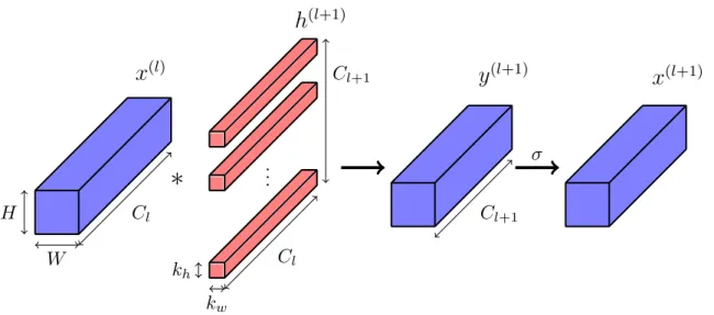
In the analysis of neural networks so far, we have considered column vectors x(l)_{, y}(l)_∈_RCl.

Convolutional layers for image analysis have a different format, with the spatial component of the input is preserved.