http://researchcommons.waikato.ac.nz/
Research Commons at the University of Waikato
Copyright Statement:
The digital copy of this thesis is protected by the Copyright Act 1994 (New Zealand). The thesis may be consulted by you, provided you comply with the provisions of the Act and the following conditions of use:
Any use you make of these documents or images must be for research or private study purposes only, and you may not make them available to any other person. Authors control the copyright of their thesis. You will recognise the author’s right
to be identified as the author of the thesis, and due acknowledgement will be made to the author where appropriate.
You will obtain the author’s permission before publishing any material from the thesis.
Knowledge for Twitter Sentiment
Analysis
A thesis
submitted in partial fulfillment of the requirements for the degree
of
Doctor of Philosophy
at
The University of Waikato
by
Felipe Bravo Márquez
Department of Computer Science Hamilton, New Zealand
July, 2017
The most popular sentiment analysis task in Twitter is the automatic classification of tweets into sentiment categories such as positive, negative, and neutral. State-of-the-art solutions to this problem are based on supervised machine learning models trained from manually annotated examples. These models are affected by label spar-sity, because the manual annotation of tweets is labour-intensive and time-consuming. This thesis addresses the label sparsity problem for Twitter polarity classification by automatically building two type of resources that can be exploited when labelled data is scarce: opinion lexicons, which are lists of words labelled by sentiment, and synthetically labelled tweets.
In the first part of the thesis, we induce Twitter-specific opinion lexicons by training words level classifiers using representations that exploit different sources of infor-mation: (a) the morphological information conveyed by part-of-speech (POS) tags, (b) associations between words and the sentiment expressed in the tweets that contain them, and (c) distributional representations calculated from unlabelled tweets. Ex-perimental results show that the induced lexicons produce significant improvements over existing manually annotated lexicons for tweet-level polarity classification.
In the second part of the thesis, we develop distant supervision methods for gener-ating synthetic training data for Twitter polarity classification by exploiting unlabelled tweets and prior lexical knowledge. Positive and negative training instances are gen-erated by averaging unlabelled tweets annotated according to a given polarity lexicon. We study different mechanisms for selecting the candidate tweets to be averaged. Our experimental results show that the training data generated by the proposed mod-els produce classifiers that perform significantly better than classifiers trained from tweets annotated with emoticons, a popular distant supervision approach for Twitter sentiment analysis.
I want to start this acknowledgment section with a story. In October 2012, I at-tended SPIRE, an information retrieval conference in Cartagena, Colombia, to present some work related to my master’s thesis. One of the keynotes was Ian Witten from the University of Waikato, who I knew quite well from the WEKA workbench and the data mining book. We had a brief chat where he asked me about my future plans. I told him I was looking for a PhD program and he suggested the University of Waikato in New Zealand. Since that moment, the idea of moving to New Zealand was seeded into my mind.
Back in Chile, I contacted Eibe Frank from the machine learning lab at Waikato University via email. He asked me what sort of topic I wanted to investigate for a potential PhD thesis, to what I replied some vague ideas about doing sentiment analysis on Twitter streams.
Only a small fraction of the emails we receive are really important. From this small fraction there is an even smaller fraction capable of triggering significant changes in our lives. On the 18th of December of 2012 I received one of those life changing emails from Bernhard Pfahringer, from which I quote the following sentence: “I’d be very keen to supervise you on a PhD doing sentiment extraction on Twitter streams or similar”.
It took a whole year of paperwork and application forms to make my trip to New Zealand possible. One day of that year, I visited the library of the University of Chile and took a copy of the data mining book authored by Witten and Frank. The last sentence of the acknowledgement section captured my attention. The sentence talked about how New Zealand had brought the authors and their corresponding families together and provided an ideal, even idyllic place to do that work.
Another life-changing email came up on the 17th of December of 2013. This time the sender was Gwenda from the Scholarships office of the University of Waikato. I was finally reading the sentence I was anxiously waiting to read: “We are delighted to inform you that your application for a Doctoral Scholarship has been successful.” Constanza came to my place one hour later, we knew that our dream of living overseas was more real than ever.
Now, I find myself, some years later, writing the acknowledgements section of my PhD thesis. I am in the the same lab where the WEKA workbench and the data mining book were created. On my desk lies a copy of the recently printed fourth edition of the book. I am happily surprised to find my name mentioned in the acknowledgement section of this new edition. The final sentence of that section is still the same of the version I read years ago at the library in the University of Chile. This time it is me who can confirm with certainty that our machine learning lab in New Zealand was an idyllic place to work on the thesis you are reading right now.
First to Constanza, my partner who crossed the Pacific Ocean with me to make this dream possible. Living together in New Zealand has been the most rewarding expe-rience of my life. I also want to express my gratitude to my parents who supported me from a distance in every aspect during all this period. This work is dedicated to you. My siblings, my extended family, and my close friends from Chile also deserve my gratitude.
I am thankful to my supervisors Bernhard Pfahringer and Eibe Frank who did an
outstanding job supervising this thesis. They both were always available when I
knocked on their doors, providing insightful guidance, allowing me to explore my own ideas, and furthermore their solid background in machine learning and programming was a permanent support for putting these ideas into practice. Thanks to Bernhard for giving me the chance of doing a PhD without even knowing me, and to Eibe for the thorough proofreading of all my drafts. I hope to follow your example if I have the chance to supervise someone someday.
I would like to thank all members of the Machine Learning group and all the visitors who made this a rewarding place to work, especially Brian Hardyment for being a true and supportive friend.
I want to express my gratitude to other good new friends I met in New Zealand outside academia: Juancho Martínez and Irina Goethe. Thanks a lot for the good moments we spent with Constanza with each of you and your corresponding families. I want also thank to Saif Mohammad from NRC Canada. Thank you for sharing your NLP expertise and for being an excellent host when I visited you in Canada.
I would also like to thank the examiners of this thesis, Cécile Paris and Mike Thel-wall, for taking the time of reading this thesis and for their valuable comments.
I want to thank all the anonymous reviewers of the papers submitted in this work, even those of the rejected ones. Many of the experiments you will find in this thesis were suggested by them.
I want to thank my former mentors and colleagues from Chile: Marcelo Mendoza, Bárbara Poblete, Claudio Gutiérrez, Mauricio Marín, Gastón L’huillier, Sebastián Ríos, and Juan Velásquez.
Even though he did not participate much in my PhD work, I am very thankful to Ian Witten, who initiated this aventure by suggesting the University of Waikato as a place for doing my PhD.
Last but not least, I would like to thank the financial support of the University of Waikato Doctoral Scholarship, and the machine learning group who funded all my conference trips.
1 Introduction 1
1.1 Twitter . . . 2
1.2 Classification . . . 3
1.2.1 Logistic Regression Models . . . 3
1.2.2 Support Vector Machines . . . 5
1.3 Research Problem . . . 7
1.4 Existing Solutions and their Limitations . . . 9
1.5 Research Proposal . . . 10
1.5.1 Word-sentiment Associations . . . 11
1.5.2 Tweet Centroid Model for Lexicon Induction . . . 12
1.5.3 Partitioned Tweet Centroids for Distant Superivison . . . . 13
1.5.4 Annotate-Sample-Average . . . 13
1.6 Publications . . . 14
1.7 Experimental Methodology . . . 15
1.7.1 Evaluation Measures . . . 16
1.8 Thesis Outline . . . 19
2 Sentiment Analysis and Social Media 21 2.1 Primary Definitions . . . 21
2.2 Sentiment Classification of Documents, Sentences, and Tweets . . 23
2.2.1 Supervised Approaches . . . 23
2.2.2 Lexicon-based Approaches . . . 26
2.2.3 Subjectivity Detection . . . 28
2.2.4 Multi-Domain Sentiment Classification . . . 28
2.2.5 Twitter Sentiment Analysis . . . 32
2.3 Polarity Lexicon Induction . . . 40
2.3.2 Corpus-based approaches . . . 42
2.4 Lexical Resources for Sentiment Analysis . . . 45
2.4.1 Comparison of Lexicons . . . 48
2.5 Analysis of Aggregated Social Media Opinions . . . 52
2.5.1 Temporal Aspects of Opinions . . . 52
2.5.2 Predictions using Social Media . . . 54
2.6 Discussion . . . 56
3 Word-sentiment Associations for Lexicon Induction 59 3.1 Proposed Method . . . 61
3.1.1 Automatically-annotated Tweets . . . 62
3.1.2 Word-level Features . . . 66
3.1.3 Ground-Truth Word Polarities . . . 69
3.2 Evaluation . . . 70
3.2.1 Exploratory Analysis . . . 70
3.2.2 Word-level Classification . . . 73
3.2.3 Lexicon expansion . . . 80
3.2.4 Extrinsic Evaluation of the Expanded Lexicons . . . 81
3.3 Discussion . . . 86
4 Distributional Models for Affective Lexicon Induction 89 4.1 Polarity Lexicon Induction with Tweet Centroids . . . 90
4.1.1 Tweet Centroids and Word-Context Matrices . . . 91
4.1.2 Evaluation . . . 93
4.2 Inducing Word–Emotion Associations by Multi-label Classification 99 4.2.1 Multi-label Classification of Words into Emotions . . . 101
4.2.2 Evaluation . . . 102
4.3 Discussion . . . 108
5 Transferring Sentiment Knowledge between Words and Tweets 111 5.1 Tweet-Centroids for Transfer learning . . . 113
5.2 Experiments . . . 116
5.2.1 The word-tweet sentiment interdependence relation . . . . 116
5.2.3 From tweets to opinion words . . . 122
5.3 Discussion . . . 125
6 Lexicon-based Distant Supervision: Annotate-Sample-Average 127 6.1 The Annotate-Sample-Average Algorithm . . . 128
6.2 ASA and The Tweet Centroid Model . . . 133
6.3 The Lexical Polarity Hypothesis . . . 135
6.4 Classification Experiments . . . 137 6.4.1 Sensitivity Analysis . . . 141 6.4.2 Learning Curves . . . 142 6.4.3 Qualitative Analysis . . . 144 6.5 Discussion . . . 145 7 Conclusions 147 7.1 Summary of Results . . . 147 7.2 Contributions . . . 149 7.3 Future Work . . . 150
7.3.1 Extensions to the Word-Sentiment Association Method . . . 150
7.3.2 Extensions to the Tweet Centroid Model . . . 150
7.3.3 Extensions to ASA . . . 152
2.1 Venn diagrams of the overlap between opinion lexicons. a) lexicons
created manually, and b) lexicons created automatically. . . 49
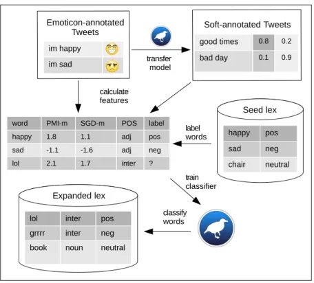
3.1 Twitter-lexicon induction process. The bird represents the Weka ma-chine learning software. . . 62
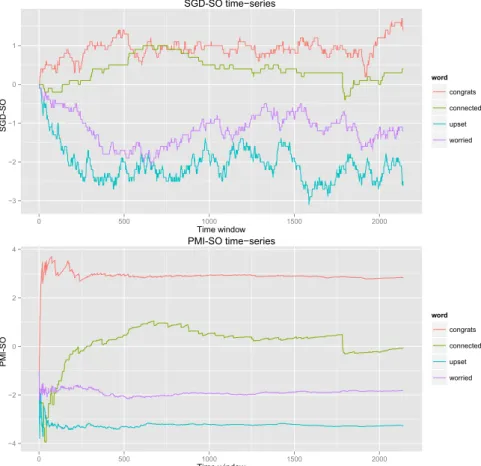
3.2 Word-level time series. . . 71
3.3 PMI-SO vs SGD-SO scatterplot. . . 74
3.4 PMI-SO and SGD-SO Boxplots. . . 75
3.5 Word clouds of positive and negative words using log odds propor-tions. . . 81
4.1 Twitter-lexicon induction with tweet centroids. The bird represents the Weka machine learning software. . . 92
4.2 Emotion classification results obtained using word embeddings of different dimensionalities, generated from various window sizes. Max-imum F1 is achieved for 400 by 5. . . 104
4.3 A visualisation for the expanded emotion lexicon. . . 106
5.1 Transfer Learning with tweet centroids. The bird represents the Weka machine learning software. . . 112
5.2 Violin plots of the polarity of tweets and words. . . 118
5.3 Word clouds of positive and negative words obtained from a message-level classifier. . . 124
6.1 Polarity distributions ofposT andnegT. . . 136
6.2 Heatmap of ASA parameters on the SemEval dataset. The highest F1 value form=F is 0.76 (a = 10, instances = 200), and form=T is 0.74 (a = 5, instances = 20). The highest AUC values for m=F and m=T occur with the same configurations as the highest values for F1 and are 0.85 and 0.81, respectively. . . 142
1.1 Classification confusion matrix. . . 17
2.1 Positive and negative emoticons. . . 33
2.2 Intersection of words. . . 49
2.3 Neutrality and uniqueness of each Lexicon. The lexicons are cate-gorised according to the annotation mechanism. . . 50
2.4 Agreement of lexicons. . . 51
2.5 Sentiment values for different words. The scores in the SWN3 col-umn correspond to the difference between the positive and nega-tive probabilities assigned by SWN3 to the word. . . 52
3.1 Emoticon-annotated datasets. . . 64
3.2 Model transfer datasets with different threshold values. . . 66
3.3 Time series features. . . 68
3.4 Lexicon Statistics. . . 70
3.5 Word-level polarity classification datasets. . . 72
3.6 Word-level feature example. . . 73
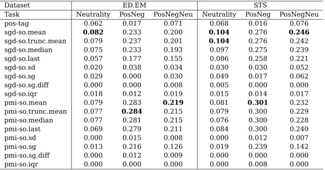
3.7 Information gain values. Best result per column is given in bold. . . 76
3.8 World-level classification performance with emoticon-based anno-tation. Best result per row is given in bold. . . 77
3.9 Word classification performance using model transfer. Best result per column is given in bold. . . 78
3.10 World-level classification performance using model transfer. Best result per row is given in bold. . . 79
3.11 Example list of words in expanded lexicon. . . 80
3.12 Message-level polarity classification datasets. . . 82
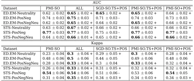
3.13 Message-level polarity classification performance. Best result per column is given in bold. . . 84
3.14 Message-level polarity classification performance with outlier re-moval. Best result per columns is given in bold. . . 86
4.1 Dataset properties. . . 94
4.2 Word-level 2-class polarity classification performance. . . 94
4.3 Word-level three-class polarity classification performance. . . 95
4.4 Intrinsic Evaluation of tweet centroids and PPMI for lexicon induc-tion. . . 96
4.5 Example of induced words. . . 97
4.6 Message-level classification performance. . . 98
4.7 Extrinsic Evaluation of TCM and PPMI for lexicon induction. . . 99
4.8 Word-level multi-label classification results. Best results per col-umn for each performance measure are shown in bold. The sym-bol + corresponds to statistically significant improvements with re-spect to the baseline. . . 105
4.9 Message-level classification results over the Hashtag Emotion Cor-pus. Best results per column are given in bold. . . 107
5.1 Average number of positive and negative instances generated by different models from 10 collections of 2 million tweets. . . 121
5.2 Message-level Polarity Classification AUC values. Best results per column are given in bold. . . 121
5.3 Number of positive and negative words from AFINN. . . 123
5.4 Word-level polarity classification results for the AFINN lexicon. Best results per row are given in bold. . . 123
6.1 Probabilities of sampling a majority of tweets with the desired po-larity. . . 132
6.2 Average number of positive and negative instances generated by different distant supervision models from 10 collections of 2 million tweets. . . 138
6.3 Macro-averaged F1 and AUC measures for different distant super-vision models. Best results per column for each measure are given in bold. . . 139
6.4 Examples of tweets classified with ASA. Positive and negative words from AFINN are marked with blue and red colours respectively. The leftmost column indicates the classifier’s output. . . 144
Introduction
Social media platforms and, in particular, microblogging services1 such as
Twitter2, Tumblr3, and Weibo4 are increasingly being adopted by users to
access and publish information about a great variety of topics. These new mediums of expression enable people to connect to each other, and voice their opinion in a simple manner (Jansen, Zhang, Sobel and Chowdury, 2009).
Sentiment analysis or opinion mining refers to the application of techniques from fields such as natural language processing (NLP), information retrieval and machine learning, to identify and extract subjective information from tex-tual datasets (Pang and Lee, 2008). One of the most popular sentiment anal-ysis tasks is the automatic classification of documents or sentences into sen-timent categories such as positive, negative, and neutral. These sensen-timent classes represent the writer’s sentiment toward the topic addressed in the message.
Sentiment analysis applied to social media platforms has received increasing interest from the research community due to its importance in a wide range of fields such as business, sports, and politics. Several works claim that so-cial phenomena such as stock prices, movie box-office revenues, and political elections, are reflected by social media data (Bollen, Mao and Zeng, 2011; Asur and Huberman, 2010; Gayo-Avello, 2013) and that opinions expressed in those platforms can be used to assess the public opinion indirectly (O’Connor, Balasubramanyan, Routledge and Smith, 2010).
This thesis focuses on analysing the sentiment of Twitter data. We use Twit-ter because it is the most widely-used microblogging service and provides large amounts of freely available public data. We propose machine
learning-1http://en.wikipedia.org/wiki/Microblogging 2http://www.twitter.com
3http://www.tumblr.com 4http://www.weibo.com
based models to tackle two sentiment analysis tasks: 1) classifying Twitter words into sentiment categories, and 2) training message-level polarity classi-fiers from unlabelled messages.
The remainder of this chapter is organised as follows. Section 1.1 presents a brief description of Twitter. Section 1.2 introduces the supervised machine learning methods used in this thesis. Section 1.3 states the research prob-lem that it addresses. Existing solutions to the probprob-lem and their limitations are briefly presented in Section 1.4. The research proposal and the proposed methods are introduced in Section 1.5. The publications derived from this work are listed in Section 1.6. The experimental methodology used to eval-uate the methods is presented in Section 1.7. In Section 1.8, we present an outline of the thesis’ structure.
1.1 Twitter
Twitter is a microblogging service founded in 2006, in which users post
mes-sages ortweets. It was originally designed to be an SMS-based service where
messages are restricted to 160 characters. Thus, tweets are limited to 140 characters, leaving 20 characters for the username. Twitter users may sub-scribe to the tweets posted by other users, an action referred to as “following”. The service can be accessed through the Twitter website or through applica-tions for smartphones and tablets.
Twitter users have adopted different conventions such as replies, retweets,
and hashtags in their tweets. Twitter replies, denoted as @username, indicate
that the tweet is a response to a tweet posted by another user. Retweets are
used to re-publish the content of another tweet using the formatRT @username.
Hashtags are used to denote the context of the message by prefixing a word with a hash symbol e.g., #obama, #elections, etc. The size restriction and con-tent sharing mechanisms of Twitter have created a unique dialect (Hu, Tala-madupula and Kambhampati, 2013) that includes many abbreviations, acronyms, misspelled words, and emoticons that are not usual in traditional media, e.g., omg, loove, or :). Words and phrases that are frequently used during a par-ticular time period are known as “trending topics”. These topics are listed by the platform for different regions of the world, and can also be personalised to the user5.
Twitter has become the most popular microblogging platform with hundreds
of millions of users spreading millions of personal posts on a daily basis6. The
rich and great volume of data propagated in it offers many opportunities for the study of public opinion and for analysing consumer trends (Jansen et al., 2009). Tweets published by public accounts can be freely retrieved using one
of the two Twitter APIs: 1) the REST search API7, which allows the submission
of queries composed of key terms, and 2) the streaming API8, from which a
real-time sample of public posts can be retrieved. These APIs enable retrieval of domain-specific tweets restricted to certain words, users, geographical lo-cation, or time periods, in order to analyse tweets associated with a particular event or population sample.
1.2 Classification
Classification is the task of predicting a discrete variable y with L possible
categories from examples represented by a set of features or independent
variables x1, x2, . . . , xn in a feature space X. In order to train a classifier we
need to learn a hypothesis functionf from a collection ofN training examples.
This collection of records has the form(X, Y), and is usually referred to as the
training dataset. Each entry of the dataset is a tuple(x, y), where xis the
fea-ture vector andyis the class or target label. When the possible outcomes ofy
are restricted to binary values,yi ∈ {+1,−1},∀i∈ {1, . . . , N}, the classification
problem is referred to as a binary classification problem.
The process of learning a hypothesis function from a training dataset is
re-ferred to as supervised learning, and there exist many machine learning
al-gorithms for training such functions, many of which are described in (Witten, Frank and Hall, 2011). The methods used in this thesis are logistic regression models and support vector machines (SVMs), because they are known to per-form well on text classification problems (Manning, Raghavan and Schütze, 2008).
1.2.1 Logistic Regression Models
Logistic regression models estimate the posterior probability P(y|x) of a
bi-nary target variable ygiven the observed values of xby fitting a linear model
to the data. The parameters of the model are formed by a vector of parameters
w, which is related to the feature spaceX by a linear function. Assuming the
6https://about.twitter.com/company 7https://dev.twitter.com/rest/public/search 8https://dev.twitter.com/streaming/overview
intercept term is x0 = 1, the linear function has the following form: hw(x) = n X i=0 wixi =wTx (1.1)
This function hw(x) is mapped into the interval [0,1] using the logistic or
sigmoid function:
g(z) = 1
1 +e−z (1.2)
In ridge logistic regression, which is the method applied in this thesis,
pa-rameters w are determined by minimising the following L2-regularised loss
function from a given training dataset ofN examples:
min w N X i=1 log(1 +e−yiwTxi) + λ 2w Tw (1.3)
The expression log(1 +e−yiwTxi)corresponds to the log-likelihood of a
prob-abilistic model in which y given x follows a Bernoulli distribution, and the
parameter λ (λ ≥ 0) is a user-specified regularisation parameter. Several
al-gorithms can be used for optimisingw given a training dataset. In this thesis
we use the trust region Newton method (Lin, Weng and Keerthi, 2008)
imple-mented in theLibLinear library (Fan, Chang, Hsieh, Wang and Lin, 2008). This
implementation scales well to large datasets and high-dimensional feature-spaces.
Once the parameters are estimated, the posterior probability of a testing example is calculated according to the following expression:
P(y|x) = 1
1 +e−wTx (1.4)
The classification output is obtained by imposing a decision threshold on the
posterior probability which is normally0.5.
Logistic regression for multi-class classification, called multinomial logistic
regression, uses thesoftmax function instead of the sigmoid function:
σ(z)j =
ezj
PK
k=1ezk
forj ∈ {1, . . . , L}. (1.5)
class9. The posterior distribution ofxfor classj is calculated as follows: P(y=j|x) = e wT jx PL l=1ew T lx (1.6) The example is normally classified into the class with the highest probability. Another approach for applying logistic regressions to multi-class problems,
which is the one implemented inLibLinear and used in this thesis, is the
one-vs-the-rest strategy proposed in (Crammer and Singer, 2002). In this strategy, a single classifier is trained per class, using the examples of that class as the positive instances and the remaining ones as the negative instances.
1.2.2 Support Vector Machines
A support vector machine (SVM) is a binary classifier aimed at finding a
large-margin hyperplane (ωT ·x+b) that separates the two class valuesy ∈ {+1,−1}
according to the feature space represented by x. If the data is linearly
sepa-rable, the optimal hyperplane is the one that maximises the margin between
positive and negative observations in the training dataset formed byN
obser-vations. In the general case, the task of learning an SVM from a dataset is formalised as the following optimisation problem:
min w,b 1 2w Tw+C N X i ξi subject to yi(wTxi+b)≥1−ξi,∀i∈ {1, . . . , N} ξi ≥0∀i∈ {1, . . . , N} (1.7)
The objective function of the problem combines the length of the parameter
vector and the errorsPN
i ξi. The parameterCis referred to as the “soft margin
regularization parameter” and controls the sensitivity of the SVM to possible outliers.
It is also possible to make SVMs find non-linear patterns efficiently using
the kernel trick. A function φ(x) that maps the feature space x into a
high-dimensional space is used. This high-high-dimensional space is a Hilbert space, and
the dot productφ(x)·φ(x0)can be represented as a kernel function K(x, x0). A
9In actual implementations, the parameter vector for one of the classes can be dropped because it is redundant.
popular kernel function is the radial basis function kernel (RBF): K(x, x0) = exp −||x−x 0||2 2σ2 (1.8)
in which σ (σ > 0) is a free parameter that has to be tuned for each specific
problem.
By using kernels, the hyperplane is calculated in the high-dimensional space
(ωT ·φ(x) +b). The dual formulation of the SVM allows replacing every dot
product by a kernel function as is shown in the following expression:
max α N X i=1 αi− 1 2 N X i,j=1 αiαjyiyj·K(xi, xj) subject to 0≤αi ≤C,∀i∈ {1, . . . , N} N X i=1 αiyi = 0 (1.9)
where the parametersαi, i∈ {1, . . . , N}correspond to the Lagrange
multipli-ers of the constrained optimisation problem. A popular algorithm for solving this quadratic programming problem is sequential minimal optimisation (Platt,
1998). In this thesis we use the implementation provided by the LIBSVM
li-brary (Chang and Lin, 2011). Once the parametersαhave been determined, it
is possible to classify a new observation xj according to the following
expres-sion: sign N X i=1 αiyi ·K(xi, xj) +b ! (1.10)
The calculation of the bias term b varies according to the the solver
algo-rithm (Platt, 1998). A convenient property of SVMs is that the values of α
will be different from zero only for a certain (usually small) number exam-ples known as support vectors. Thus, SVMs only need to evaluate the kernel
function between xj and the support vectors.
SVMs can also be applied to multi-class problems, e.g., by using the one-vs-the-rest strategy introduced in the previous section.
1.3 Research Problem
We refer to message-level polarity classification as the task of automatically classifying tweets into sentiment categories. This problem has been success-fully tackled by representing tweets from a corpus of hand-annotated exam-ples using feature vectors and training classification algorithms on them (Mo-hammad, Kiritchenko and Zhu, 2013). A popular choice for building the
fea-ture space X is the vector space model (Salton, Wong and Yang, 1975), in
which all the different words or unigrams found in the corpus are mapped
into individual features. Word n-grams, which are consecutive sequences of
n words, can also been used analogously. Each tweet is represented as a
sparse vector whose active dimensions (dimensions that are different from
zero) correspond to the words orn-grams found in the message. The values of
each active dimension can be calculated using different weighting schemes, such as binary weights or frequency-based weights with different normalisa-tion schemes.
The message-level sentiment label spaceY corresponds to the different
sen-timent categories that can be expressed in a tweet, e.g., positive, negative, and neutral. Because sentiment is a subjective judgment, the ground-truth sentiment category of a tweet must be determined by a human evaluator, and hence, the manual annotation of tweets into sentiment classes is a time-consuming and labour-intensive task. We refer to this problem as the label sparsity problem. Because supervised machine learning models are imprac-tical in the absence of labelled tweets, the label sparsity problem imposes practical limitations on using these techniques for classifying the sentiment of tweets.
Crowdsourcing tools such as Amazon Mechanical Turk10 or CrowdFlower11
allow clients to use human intelligence to perform tasks in exchange for a monetary payment set by the client. They have been successfully used for manually labelling tweets into sentiment classes (Nakov, Rosenthal, Kozareva, Stoyanov, Ritter and Wilson, 2013). Nevertheless, a classifier trained from a particular collection of manually annotated tweets will not necessarily perform well on tweets about topics that were not included in the training data or on tweets written in a different period of time. This is because the relation between messages and the corresponding sentiment label can change from one domain to another or over time. We refer to this problem as the sentiment
10https://www.mturk.com 11https://www.crowdflower.com
drift problem.
Social media opinions are expressed in different domains such as politics, products, movie reviews, sports, among others. More specifically, opinions are expressed about particular topics, entities or subjects of a certain domain. For example, “Barack Obama” is a specific entity of the domain “politics”.
The words and expressions that define the sentiment of a text passage are
referred to in the literature asopinion words (Liu, 2012). For instance,happy
is a positive opinion word and sad is a negative one. As has been studied
in (Engström, 2004; Read, 2005) many opinion words are domain-dependent. That means that words or expressions that are considered as positive or neg-ative for a certain domain will not necessarily have the same relevance or orientation in a different context. This situation is clarified in the following examples taken from real posts on Twitter:
1. For me the queue was pretty small and it was only a 20 minute wait I
think but was so worth it!!! :D @raynwise
2. Odd spatiality in Stuttgart. Hotel room is so small I can barely turn
around but surroundings are inhumanly vast & long under construction.
3. My girlfriend just called me to say good night because sheaccident(sic)
fell asleep without saying it earlier :) #ShesTooCute
4. I got some RAGE over this #Harambeaccident. This is why there should
be NO zoos.
Here we can see that opinion words small and accident can be used to
express opposite sentiment in different contexts. This is a manifestation of the sentiment drift problem, and its main consequence is that a sentiment classifier that was trained on data of a particular domain may not necessarily have the same classification performance for other topics or domains.
Temporal changes in the sentiment pattern are another manifestation of sen-timent drift. The relation between messages and their corresponding senti-ment label for a particular topic is non-stationary, i.e., it can change over time (Durant and Smith, 2007; Bifet and Frank, 2010; Bifet, Holmes and Pfahringer, 2011; Silva, Gomide, Veloso, Meira and Ferreira, 2011; Calais Guerra, Veloso, Meira Jr and Almeida, 2011; Guerra, Meira and Cardie, 2014). For instance, when an unexpected event associated with the topic occurs suddenly (e.g., a scandal linked to a public figure), new expressions conveying sentiment
can arise spontaneously, such as #trumpwall and #PrayForParis. Addition-ally, other existing words or expressions can change their frequency affecting the polarity pattern of the topic. Hence, the accuracy of a sentiment classifier affected by this change would decrease over time.
This problem was empirically studied in (Durant and Smith, 2007) by train-ing sentiment classifiers ustrain-ing traintrain-ing and testtrain-ing data from different time periods. The results indicated a significant decrease in the classification per-formance as the time difference between the training and the testing data was increased.
A possible approach to overcome the sentiment drift problem is to constantly update the sentiment classifier with new labelled data (Silva et al., 2011). However, as discussed in (Silva et al., 2011; Calais Guerra et al., 2011; Guerra et al., 2014), the high volume and sparsity of social streams make the continu-ous acquisition of sentiment labels, even using crowdsourcing tools, infeasible. The label sparsity and sentiment drift problems are connected.
The research problem considered in this thesis is how to derive accurate polarity classifiers for Twitter in label sparsity conditions without relying on the costly process of human annotation.
1.4 Existing Solutions and their Limitations
Opinion lexicons are a well known type of resource for supporting sentiment analysis of documents, especially when sentiment-annotated documents are
scarce. An opinion lexicon is a list of terms oropinion wordsannotated
accord-ing to sentiment categories such as positive and negative. Opinion lexicons can be used as prior lexical knowledge for calculating the sentiment of doc-uments and tweets in an unsupervised fashion (Hatzivassiloglou and Wiebe, 2000; Taboada, Brooke, Tofiloski, Voll and Stede, 2011; Thelwall, Buckley and Paltoglou, 2012), and to extract low-dimensional message-level features, such as the number of words in the message matching each sentiment category, for training sentiment classifiers from small samples of annotated data (Bravo-Marquez, Mendoza and Poblete, 2014; Kouloumpis, Wilson and Moore, 2011; Mohammad et al., 2013; Jiang, Yu, Zhou, Liu and Zhao, 2011).
Opinion lexicons, however, suffer from similar shortcomings as supervised models for classifying the sentiment of tweets. The ground-truth sentiment of a word is a subjective judgment determined by a human, and the diversity of informal expressions found in Twitter makes the manually annotation of opin-ion words also an expensive and time-consuming task. Furthermore, opinopin-ion
lexicons are not immune to the sentiment drift phenomenon. Some word polar-ities can be inaccurate for certain domains, and they can also become obsolete due to temporal changes in the sentiment pattern.
An appealing strategy to address both the label sparsity and sentiment drift problems for message-level polarity classification in Twitter is distant super-vision. Distant supervision models are heuristic labelling functions (Mintz, Bills, Snow and Jurafsky, 2009) used for automatically creating training data from unlabelled corpora. These models have been widely adopted for Twitter sentiment analysis because large amounts of unlabelled tweets can be easily obtained through the use of the Twitter API.
Theoretically speaking, distant supervision is a direct solution to the label sparsity problem as it replaces the human annotation labour. It can also po-tentially solve the sentiment drift problem because existing classifiers can be updated with more recently labelled examples or with tweets annotated from the domain in which a drift is being observed.
A well-known distant supervision approach for Twitter polarity classifica-tion is the emoticon-annotaclassifica-tion approach, in which tweets with positive :) or negative :( emoticons are labelled according to the polarity indicated by the emoticon after removing the emoticon from the content (Read, 2005). This method is affected by the following limitations:
1. The removal of all tweets without emoticons may cause a loss of valuable information.
2. Emoticons are likely to produce misleading labels such as in the following
example: “you’re not dating me? sad... tragic... for you at least :)”,
3. There are many domains such as politics, in which emoticons are not frequently used to express positive and negative opinions, and hence, it is very difficult to obtain emoticon-annotated data from these domains. As we can see, existing methods based on opinion lexicons and distant su-pervision exhibit major drawbacks when used for classifying the sentiment of tweets in label sparsity conditions.
1.5 Research Proposal
This thesis addresses the label sparsity problem for Twitter polarity classifica-tion by acquiring and exploiting lexical knowledge. The research hypothesis is as follows:
“Polarity classification of tweets when training data is sparse can be successfully tackled through Twitter-specific polarity lexicons and lexicon-based distant supervision.”
The problem of acquiring lexical knowledge in the form of opinion lexicons is referred to as polarity lexicon induction. We propose two Twitter-specific polarity lexicon induction methods based on level classification: 1) word-sentiment associations and 2) the tweet centroid model. We also propose two distant supervision methods that exploit existing opinion lexicons for building synthetically labelled data on which message-level polarity classifiers can be trained: 1) partitioned tweet centroids and 2) annotate-sample-average (ASA). We now briefly review these methods.
1.5.1 Word-sentiment Associations
This method combines information from automatically annotated tweets and existing hand-made opinion lexicons to induce a Twitter-specific opinion lexi-con in a supervised fashion. The induced lexilexi-con lexi-contains part-of-speech (POS) disambiguated entries (e.g., noun, verb, adjective) with a probability distribu-tion for positive, negative, and neutral polarity classes.
To obtain this distribution using machine learning, word-level attributes are used based on (a) the morphological information conveyed by POS tags and (b) associations between words and the sentiment expressed in the tweets that contain them. The sentiment associations are modelled in two different ways: using point-wise-mutual-information semantic orientation (PMI-SO) (Turney, 2002), which is based on the point-wise mutual information between a word and tweet-level polarity classes, and using stochastic gradient descent seman-tic orientation (SGD-SO), which learns a linear relationship between words and sentiment.
The message-level sentiment labels are obtained automatically using emoti-cons and a transfer learning approach. The transfer learning approach en-ables learning of opinion words from tweets without emoticons by deploying a message-level classifier trained from tweets annotated with emoticons on a target collection of unlabelled tweets.
The training words are labelled by a seed lexicon formed by combining mul-tiple hand-annotated lexicons, and the induced lexicon is obtained after de-ploying the trained word-level classifier on the remaining unlabelled words
from the corpus of tweets.
The experimental results show that the method outperforms the word-level
polarity classification performance obtained by using PMI-SO alone. This
is significant because PMI-SO is a state-of-the-art measure for establishing world-level sentiment.
1.5.2 Tweet Centroid Model for Lexicon Induction
The tweet centroid model is another word-level classification model for po-larity lexicon induction, which in contrast to the previous method, does not necessarily depend on labelled tweets and can perform lexicon induction di-rectly from a given corpus of unlabelled tweets.
The distributional hypothesis (Harris, 1954) states that words occurring in similar contexts have similar meanings. Distributional semantic models (Tur-ney and Pantel, 2010) are used for representing lexical items such as words according to the context in which they occur. The tweet centroid model is a distributional representation that exploits the short nature of tweets by treat-ing them as the whole contexts of words. In the tweet centroid model, tweets are represented by sparse vectors using standard natural language process-ing (NLP) features, such as unigrams and low-dimensional word-clusters, and words are represented as the centroids of the tweet vectors in which they appear.
The lexicon induction is conducted by training a word-level classifier using these centroids to form the instance space and a seed lexicon to label the train-ing instances. The trained classifier is deployed on the remaintrain-ing unlabelled words in the same way as in the previous model.
Experimental results show lexicons generated with the tweet centroid model produce valuable features for classifying the sentiment of tweets when com-pared with the original seed lexicon.
The model is also used to produce a more fine-grained word-level categori-sation based on emotion categories, e.g., anger, fear, surprise, and joy. This is done by employing labels provided by an emotion-associated lexicon (Moham-mad and Turney, 2013) and multi-label classification techniques.
The tweet centroid model allows message-level classifiers trained from sentiment-annotated tweets to be deployed on words for polarity lexicon induction be-cause both tweets and words are represented by feature vectors of the same dimensionality and can also be labelled according to the same sentiment cate-gories, e.g, positive and negative. This is useful in scenarios where no labelled
words are available for training a word-level classifier, but labelled tweets can be obtained instead.
1.5.3 Partitioned Tweet Centroids for Distant Superivison
Lexicon-based distant supervision methods automatically create message-level training data from unlabelled tweets by exploiting the prior sentiment knowl-edge provided by opinion lexicons. As lexicons are usually formed by more than a thousand words, lexicon-based methods can potentially exploit more data than a small number of positive and negative emoticons.
The tweet centroid model can also be used as a lexicon-based distant su-pervision method. As tweets and words are represented by the same feature vectors, a word-level classifier trained from a polarity lexicon and a corpus of unlabelled tweets can be used for classifying the sentiment of tweets repre-sented by sparse feature vectors. In other words, the labelled word vectors correspond to lexicon-annotated training data for message-level polarity clas-sification.
A drawback of this simple idea is that the number of labelled words for train-ing the word-level classifier is limited to the number of words in the lexicon. In some scenarios, it is desirable to be able to create training datasets that increase in size when increasing the size of the source corpus of unlabelled tweets. This is because many classifiers perform better when trained from large datasets (Witten et al., 2011). We propose a simple modification to the tweet centroid model for increasing the number of labelled instances, yielding “partitioned tweet centroids". This modification is based on partitioning the tweets associated with each word into smaller disjoint subsets of a fixed size. The method calculates one centroid per partition, which is labelled according to the lexicon. The experimental results show that partitioned tweet centroids outperform the emoticon-annotation approach for message-level polarity clas-sification.
1.5.4 Annotate-Sample-Average
Annotate-Sample-Average (ASA) is another lexicon-based distant supervision method for training polarity classifiers in Twitter in the absence of labelled data. ASA takes a collection of unlabelled tweets and a polarity lexicon com-posed of positive and negative words and creates synthetic labelled instances for message-level polarity classification. Each labelled instance is created by
sampling with replacement a number of tweets containing at least one word from the lexicon with the desired polarity, and averaging the feature vectors of the sampled tweets.
The rationale of the method is based on the hypothesis that a tweet contain-ing an opinion word with a known polarity is more likely to express the same polarity than the opposite one. Consequently, averaging multiple tweets con-taining words with the same polarity increases the confidence of obcon-taining a vector located in the region of the target polarity.
This hypothesis is empirically validated, and the experimental results show that the training data generated by ASA (after tuning its parameters) produces a message-level classifier that performs significantly better than a classifier trained from tweets annotated with emoticons and a classifier trained, without any sampling and averaging, from tweets annotated according to the polarity of their words.
1.6 Publications
During the course of this project, the following peer-reviewed papers have been published in journals and conference proceedings:
1. F. Bravo-Marquez, E. Frank, and B. PfahringerPositive, Negative, or
Neu-tral: Learning an Expanded Opinion Lexicon from Emoticon-annotated Tweets, InIJCAI ’15: Proceedings of the 24th International Joint Confer-ence on Artificial IntelligConfer-ence. Buenos Aires, Argentina 2015.
2. F. Bravo-Marquez, E. Frank, and B. Pfahringer From Unlabelled Tweets
to Twitter-specific Opinion Words, InSIGIR ’15: Proceedings of the 38th International ACM SIGIR Conference on Research & Development in In-formation Retrieval. Santiago, Chile 2015.
3. F. Bravo-Marquez, E. Frank, and B. Pfahringer Building a Twitter
Opin-ion Lexicon from Automatically-annotated Tweets, In Knowledge-Based Systems. Volume 108, 15 September 2016, Pages 65 -– 78.
4. F. Bravo-Marquez, E. Frank, and B. PfahringerAnnotate-Sample-Average
(ASA): A New Distant Supervision Approach for Twitter Sentiment Anal-ysis, In ECAI’16: Proceedings of the biennial European Conference on Artificial Intelligence. The Hague, Netherlands 2016.
5. F. Bravo-Marquez, E. Frank, and B. PfahringerFrom opinion lexicons to sentiment classification of tweets and vice versa: a transfer learning ap-proach, In WI’16: Proceedings of the IEEE/WIC/ACM International Con-ference on Web Intelligence. Omaha, Nebraska, USA 2016.
6. F. Bravo-Marquez, E. Frank, S. Mohammad, and B. Pfahringer
Determin-ing Word–Emotion Associations from Tweets by Multi-Label Classifica-tion, In WI’16: Proceedings of the IEEE/WIC/ACM International Confer-ence on Web IntelligConfer-ence. Omaha, Nebraska, USA 2016.
1.7 Experimental Methodology
The methods proposed in this thesis are evaluated empirically on collections of manually-annotated data. We use hand-annotated lexicons as ground truth for the polarity lexicon induction methods and tweets that were manually an-notated into sentiment classes for evaluating the distant supervision methods. All these datasets are described in Chapter 2.
When evaluating a machine learning classifier, it is not recommended to carry out the evaluation on the same data on which the classifier was trained. The performance obtained on the training data is likely to be biased and mis-leadingly optimistic, because some classifiers are prone to learn random noise. This phenomenon is known as over-fitting, and is commonly addressed by eval-uating classifiers on independent testing examples that were not included for training.
In the “hold-out” approach, the training dataset is split into two independent training and testing datasets. The classifier is trained over the training set and then used to classify the values of the testing set. The predicted outputs are compared with their corresponding gold standard values.
A drawback of the “hold-out” approach is that all the examples within the testing set are not used for training purposes. As it has been discussed before, the labelled observations are often expensive to obtain, and hence it would be
better to use all the available training examples. The k-fold cross-validation
approach tackles this problem by randomly partitioning the training data into
kfolds of the same size, which are all stratified to maintain the same class
dis-tribution as the original dataset. Then, for each fold k, a classifier is trained
over the remainingk−1folds and evaluated over the retained one. The
eval-uation measures are averaged for all the folds ensuring that all observations are used for both training and evaluation purposes. Cross-validation gives a
more robust estimation of the classifier’s performance on unseen data than the “hold-out” approach, and allows estimating the standard deviation of the per-formance across the folds. Additionally, the cross-validation procedure can be repeated multiple times using different random partitions of the folds (varying the random seed number), in order to get a better estimation of the classifier’s performance.
Cross-validation can be used for statistically comparing the performance of two different classifiers on the same data. The average performance scores
produced by two classifiers for all kfolds, or n×k if the process is repeated n
times, can be compared using statistical tests such as the pairedt-student test.
The null hypothesis is that there is no difference in the average performance of two classification schemes. In this thesis, we compare different word-level and message-level sentiment classification schemes with cross-validation using the
corrected resampled pairedt-student test with anα level of0.05(Nadeau and
Bengio, 2003). This statistical test is a variant of the pairedt-student test that
corrects the problems that arise when different performance estimations are calculated from overlapping samples.
Cross-validation is not suitable for evaluating distant supervision schemes. This is because the automatically-labelled examples, such as tweets with emoti-cons, correspond to a biased sample of the real tweets (Go, Bhayani and Huang, 2009). We calculate the average performance of distant supervision classifiers deployed on an independent target collection of manually-annotated examples by varying the collection of unlabelled tweets from which the la-belled training data is generated. The performance of two distant supervision methods estimated in this way is compared using the non-parametric paired
Wilcoxon signed-rank test with the significance value set to0.05.
1.7.1 Evaluation Measures
Next, we introduce the performance metrics used for evaluating classifiers.
Considering a binary classifier f deployed on a testing dataset, four possible
outcomes can be calculated: 1) correctly classified positive observations or True Positives (TP), 2) correctly classified negative observations or True Neg-atives (TN), 3) negative observations wrongly classified as positive or False Positives (FP), and 4) positive observations wrongly classified as negative or False Negatives (FN). These outputs are normally displayed in a confusion
matrix C such as Table 1.1.
ma-y= +1 y=−1
f(x) = +1 T P F P f(x) = −1 F N T N
Table 1.1: Classification confusion matrix.
trixC whereLis the number of classes andN is the total number of examples
in the dataset. A cell Cij corresponds to the number of examples for which
the classifier predicts class i and the real class is j. Note that all correctly
classified examples lie on the diagonal of the matrix, and that the sum of all
the elements of the matrix is equal to the total number of examples (N):
N = L X i=1 L X j=1 Cij (1.11)
The evaluation measures are described below:
• Accuracy, the overall percentage of correctly classified observations. For binary classification problems, it is calculated as follows:
Accuracy= T P +T N
T P +T N +F P +F N. (1.12)
and it is generalised to multi-class problems according to the following expression:
Accuracy=
PL
i=1Cii
N (1.13)
• Kappa statistic: In classification problems in which the class distribution is highly skewed towards a majority class, a classifier can yield a high
accuracy by chance. The kappa statistic κ (Cohen, 1960) corrects this
problem by normalising the classification accuracy according to the im-balance of the classes in the data. A classifier that is always correct will
have a κ of one. Conversely, if it makes the right predictions with the
same probability as a random classifier, the value of κ will be zero. It is
calculated as follows:
κ = Accuracy−pc
1−pc
(1.14)
pc= L X i=1 L X j=1 Cij N · L X j=1 Cji N ! (1.15)
• Precision, the fraction of correctly classified positive observations over all the observations classified as positive:
Precision= T P
T P +F P. (1.16)
In multi-class problems, multiple precisions are calculated using a one-vs-the-rest strategy and averaged. It is common to weight the scores according to the relative frequency of their corresponding classes. This approach applies for all the remaining measures in multi-class scenarios.
• Recall (also called sensitivity and true positive rate), the fraction of cor-rectly classified positive observations over all the positive observations:
Recall= T P
T P +F N. (1.17)
• F1-score, the harmonic mean between the precision and recall:
F1-score= 2· Precision·Recall
Precision+Recall. (1.18)
• Area Under the Curve (AUC): The receiver operating characteristic (ROC) curve or ROC curve plots the true positive rate (TPR), which is equivalent to recall, against the false positive rate (FPR), which is calculated as fol-lows:
FPR= F P
F P +T N. (1.19)
The multiple values of TPR and FPR required for building an ROC curve are obtained using different threshold settings for a same classifier. For example, in a logistic regression model, different decision thresholds for the posterior probability are considered. The area under the ROC curve (AUC) is a useful metric because it is independent of any specific value for the decision threshold. This area is 1 for a perfect classifier and 0.5 for a random one.
1.8 Thesis Outline
This thesis is structured as follows. A review of the literature on sentiment analysis and social media is presented in Chapter 2. The word-sentiment as-sociation method for polarity lexicon induction is described and evaluated in Chapter 3. Chapter 4 describes the tweet centroid model for polarity lexicon induction and for determining word-emotion associations. In Chapter 5, the tweet centroid model is used for transferring sentiment knowledge between words and tweets. The partitioned version of the model for distant supervision is also described in that chapter. The annotate-sample-average distant super-vision method is described and evaluated in Chapter 6. Chapter 7 presents the main findings and contributions of this thesis, as well as a perspective for future work.
Sentiment Analysis and Social Media
In the early stages of the Web, its content was usually published by website owners associated with traditional information sources such as news media
and companies, among other organisations. Additionally, the content was
mainly about “facts” which are objective statements on particular entities or topics. In the 2000s, the rise of Web 2.0 platforms (O’Reilly, 2007), e.g., blogs, online social networks and microblogging services, changed this situation by allowing users to generate and share textual content in a simpler way. This situation caused an explosive growth of subjective information (i.e., personal opinions) available on the Web, which in turn provided new opportunities for information system developers. As the factual information has been tradi-tionally processed using techniques such as information retrieval and topic classification, different types of methods are required in order to process the “subjective" content generated by users. In this chapter, we give a review of those methods, which are commonly referred to in the research literature as opinion mining andsentiment analysis techniques. We discuss works address-ing sentiment classification of documents, sentences, and tweets, as well as methods for polarity lexicon induction. Popular existing opinion lexicons are also reviewed and analysed. Moreover, we discuss work conducting aggre-gated analysis of opinions and applications of sentiment analysis and social media mining, including predictions about stock market prices and election outcomes. Finally, we provide a discussion of existing developments in the field in the context of the research problem addressed in this thesis.
2.1 Primary Definitions
Letd be an opinionated document (e.g., a product review) composed of a list
of sentences s1, . . . , sn. As stated in (Liu, 2009), the basic components of an
• Entity: can be a product, person, event, organisation, or topic on which an opinion is expressed (opinion target). An entity is composed of a
hi-erarchy of components and sub-components where each component can
have a set of attributes. For example, a cell phone is composed of a
screen, a battery among other components, the attributes of which could be the size and the weight. For simplicity, components and attributes are
both referred to asaspects.
• Opinion holder: the person or organisation that holds a specific opinion
on a particular entity. While in reviews or blog posts the holders are
usually the authors of the documents, in news articles the holders are commonly indicated explicitly (Bethard, Yu, Thornton, Hatzivassiloglou and Jurafsky, 2004).
• Opinion: a view, attitude, or appraisal of anobjectfrom anopinion holder.
An opinion can have a positive, negative or neutralorientation, where the
neutral orientation is commonly interpreted as no opinion. The
orienta-tion is also named sentiment orientation, semantic orientation (Turney,
2002), orpolarity.
Considering the components of the opinions presented above, an opinion is defined as a quintuple (ei, aij, ooijkl, hk, tl) (Liu, 2010). Here, ei is an entity, aij
is an aspect of ei and ooijkl is the opinion orientation of aij expressed by the
holder hk during time period tl. Possible values for ooijkl are the categories
positive, negative and neutral or different strength/intensity levels. In cases
when the opinion refers to the whole entity, aij takes a special value named
GENERAL.
It is important to consider that within an opinionated document, several opinions about different entities and also different holders can be found. In this context, a more general opinion mining problem can be addressed consist-ing of discoverconsist-ing all opinion quintuples (ei, aij, ooijkl, hk, tl) from a collection
D of opinionated documents. These approaches are referred to as
aspect-based or feature-based opinion mining methods (Liu, 2009). As we can see, working with opinionated documents involves tasks such as identifying enti-ties, extracting aspects from the entienti-ties, the identification of opinion holders (Bethard et al., 2004), and the sentiment evaluation of the opinions (Pang and Lee, 2008).
In addition to the orientation or polarity, there are other affective dimensions
A sentence of a document is defined as subjective when it expresses personal feelings, views or beliefs. It is common to treat neutral sentences as objective and opinionated sentences as subjective.
Emotions are subjective feelings and thoughts. According to (Parrot, 2001) people have six primary emotions, which are: love, joy, surprise, anger, sad-ness, and fear. Another categorisation, proposed by Ekman (1992), is formed by 6 basic emotions: anger, fear, joy, sadness, surprise, and disgust, which was latter extended by Plutchik (2001) to include two additional emotion states: anticipation and trust.
The affective dimension of a document can be represented using different variable types. Nominal variables are used to represent hard associations with the affective dimension e.g., positive or non-positive, while ordinal and numeric variables are used to represent intensity or strength levels, such as weakly positive, strongly positive, or 40% negative.
2.2 Sentiment Classification of Documents,
Sentences, and Tweets
The most popular task in sentiment analysis is document sentiment classi-fication, which generalises the message-level polarity classification problem presented in Chapter 1 to documents of any length. A common assumption for simplifying the problem is that the target document expresses opinions about one single entity from one opinion holder (Liu, 2009). When sentiment clas-sification is applied to a single sentence instead of to a whole document, the
task is namedsentence-level sentiment classification (Wilson, Wiebe and
Hoff-mann, 2005). In this section we review five approaches to sentiment classifi-cation: 1) supervised approaches, 2) lexicon-based approaches, 3) subjectivity detection, 4) multi-domain sentiment classification, and 5) sentiment classifi-cation of tweets.
2.2.1 Supervised Approaches
A popular approach is to model the problem as a supervised learning problem. The idea behind this approach is to train a function capable of determining the sentiment orientation of an unseen document using a corpus of documents labelled by sentiment. For example, the training and testing data can be ob-tained from websites of product reviews where each review is composed of a free text comment and a reviewer-assigned rating. A list of available training
corpora from opinion reviews can be found in (Pang and Lee, 2008). After-wards, the text data and the ratings are transformed into a feature-vector and a target value respectively. For example, if the rating is on a 1-5 star scale, high-starred reviews can be labelled as positive opinions and low-starred re-views as negative in the same way. The problem can also be formulated as an ordinal regression problem using the number of stars as the target variable (Pang and Lee, 2005). In (Pang, Lee and Vaithyanathan, 2002), the authors trained a binary classifier (positive/negative) over movie reviews from the In-ternet Movie Database (IMDb). They used the following features: unigrams, bigrams, and part of speech tags, and the following learning algorithms: Sup-port Vector Machines (SVM), Maximum Entropy Classifier, and Naive Bayes. The best average classification accuracy obtained through a three-fold
cross-validation was 82.9%. This result was achieved using purely unigrams as
fea-tures and an SVM as learning algorithm.
More recent models have adopted the “representation learning” approach of learning the document representation directly from the data using neu-ral networks (Collobert and Weston, 2008). Word embeddings are a popular choice among those approaches. They are low-dimensional continuous dense word vectors trained from unlabelled document corpora capable of capturing rich semantic information. A state-of-the-art word embedding model is the skip-gram model (Mikolov, Sutskever, Chen, Corrado and Dean, 2013)
imple-mented in the Word2vec1 library. In this method, a neural network with one
hidden layer is trained for predicting the words surrounding a centre word,
within a window of size k that is shifted along the input corpus. The centre
and surroundingk words correspond to the input and output layers of the
net-work, respectively, and are represented by 1-hot vectors, which are vectors of
the size of the vocabulary (|V|) with zero values in all entries except for the
corresponding word index that receives a value of 1. Note that the output
layer is formed by the concatenation of thek 1-hot vectors of the surrounding
words. The hidden layer has a dimensionality l, which determines the size of
the embeddings (normally l |V|). The word-embedding for each word can
be obtained in two ways: 1) from the projection matrix connecting the input layer with the hidden one, and 2) from the projection matrix connecting the hidden layer with the output one. The network is efficiently trained using an algorithm called “negative-sampling”, and the rationale of the model is that words occurring in similar contexts will receive similar vectors. There is
other word embedding model called continuous bag of words (CBOW), which is analogous to the skip-gram model after swapping its input and output lay-ers. Thus, the learning task of CBOW consist of predicting a centre word given its surrounding words in a window.
A simple approach for using word-embeddings in sentence-level polarity classification is to use the average word vector as the feature representation of a sentence, which is latter used as input for training a sentence-level polarity classifier (Castellucci, Croce and Basili, 2015).
There are syntactic dependencies such as negations and but clauses known as “opinion shifters” (Liu, 2009) that can strongly alter the overall polarity of a sentence, e.g., “I didn’t like the movie”, “I like you but I’m married”. Repre-sentations based on unigrams or averaging word embeddings lack information about the sentence structure. Hence, they are unable to capture long-distance dependencies in the passage. In the following, we discuss two representation learning techniques for modelling semantic compositionality in sentences that were successfully employed for sentiment analysis.
A recursive neural tensor network for learning the sentiment of pieces of texts of different granularities, such as words, phrases, and sentences, was proposed in (Socher, Perelygin, Wu, Chuang, Manning, Ng and Potts, 2013).
The network was trained on a sentiment annotated treebank2 of parsed
sen-tences for learning compositional vectors of words and phrases. Every node in the parse tree receives a vector, and there is a matrix capturing how the meaning of adjacent nodes changes. The main drawback of this model is that it relies on parsing. Thus, it would be difficult to apply it to Twitter data because of the lack of Twitter-specific sentiment treebanks and robust constituency parsers for Twitter (Foster, Cetinoglu, Wagner, Le Roux, Nivre, Hogan and van Genabith, 2011).
A paragraph vector-embedding model that learns vectors for sequences of words of arbitrary length (e.g, sentences, paragraphs, or documents) without relying on parsing was proposed in (Le and Mikolov, 2014). The paragraph vectors are obtained by training a similar network as the one used for training the CBOW embeddings. The words surrounding a centre word in a window are used as input together with a paragraph-level vector for predict the centre word. The paragraph-vector acts as a memory token that is used for all the centre words in the paragraph during the training the phase.
The recursive neural tensor network and the paragraph-vector embedding
were evaluated on the same movie review dataset used in (Pang et al., 2002), obtaining an accuracy of 85.4% and 87.8%, respectively. Both models outper-formed the results obtained by classifiers trained on representations based on bag-of-words features.
Most sentiment analysis datasets are imbalanced in favour of positive ex-amples (Li, Wang, Zhou and Lee, 2011). This is presumably because users are more likely to report positive than negative opinions. The shortcoming of training sentiment classifiers from imbalanced datasets is that many classifica-tion algorithms tend to predict test samples as the majority class (Japkowicz and Stephen, 2002) when trained from this type of data. A semi-supervised model for imbalanced sentiment classification is proposed in (Li et al., 2011). The model exploits both labelled and unlabelled documents by iteratively per-forming under-sampling of the majority class in a co-training framework using random subspaces of features.
2.2.2 Lexicon-based Approaches
In scenarios where training data is scarce, supervised models become imprac-tical. Here we review models that exploit existing lexical knowledge about the sentiment of words for classifying the sentiment of documents.
We identify two types of lexicon-based approaches: 1) unsupervised models that do not require a training corpus of labelled documents, and 2) mixed models that combine lexical knowledge with labelled documents.
A common way of computing the polarity of a document relying only on lexicon knowledge is to aggregate the orientation values of the known opinion words found in the document (Hatzivassiloglou and Wiebe, 2000). A simple approach is to calculate the difference between positive and negative words, and label the document according to the difference’s sign. More sophisticated aggregation functions including rules for negations and opinion shifters have also been proposed (Taboada et al., 2011; Thelwall et al., 2012).
A well-known model that uses the orientation of two opinion words and co-occurrence statistics obtained from a search engine is proposed in (Turney, 2002). First of all, a part-of-speech (POS) tagging is applied to all words of the document. POS tagging automatically identifies the linguistic category to which a word belongs within a sentence. Common POS categories are: noun, verb, adjective, adverb, pronoun, preposition, conjunction and interjection. The hypothesis of this work is that phrases containing a sequence of an ad-jective or an adverb as adad-jective followed by an adverb probably express an