Quantifying uncertainty in radar rainfall estimates using an X-band dual polarisation weather radar

(1)

Quantifying uncertainty in radar rainfall

estimates using an X-band dual

polarisation weather radar

David Richard Lloyd Dufton

Submitted in accordance with the requirements for the degree of Doctor of Philosophy

The University of Leeds

School of Earth and Environment

August 2016

(2)

(3)

Declaration of Authorship

The candidate confirms that the work submitted is his own, except where work which has formed part of jointly-authored publications has been included. The contribution of the candidate and the other authors to this work has been explicitly indicated below. The candidate confirms that appropriate credit has been given within the thesis where reference has been made to the work of others.

The work in Chapter 5, Section 5.3 has appeared in publication as follows:

Fuzzy logic filtering of radar reflectivity to remove non-meteorological echoes using dual polarization radar moments: Dufton, D. R. L. and Collier, C. G., Atmospheric Measure-ment Techniques, 8, 3985-4000, 2015

David Dufton was responsible for the development of the method and the data analysis in this paper, along with its writing, submission and response to reviewers. The contribution of the other author was the addition of subject knowledge, guidance and support. This copy has been supplied on the understanding that it is copyright material and that no quotation from the thesis may be published without proper acknowledgement. ©2016 The University of Leeds and David Dufton.

The right of David Dufton to be identified as Author of this work has been asserted by him in accordance with the Copyright, Designs and Patents Act 1988.

(4)

(5)

Acknowledgements

Firstly I would like to extend my deepest thanks to my supervisors Chris Collier and Alan Blyth for their guidance and support without which my research would not have been possible. Chris’s great breadth of knowledge on radar and its hydrometeorological applications along with his excitement about all things radar has helped steer my research towards its conclusion and provided encouragement along the way. Alan has always been on hand to provide some much needed atmospheric context and his enthusiasm has always been an encouragement to persevere. Thank you both for your encouragement and all the opportunities you have provided me over the last few years.

I would also like to thank everybody involved in the COPE field campaign, particularly Lindsay Bennett who’s perseverance and determination in deploying the radar knows no bounds whatever the radar might do. Throughout my research Lindsay has always been around to muse radar and it’s myriad complications and her support and guidance has been invaluable over the course of my PhD. Thanks also to the rest of the NCAS radar group, past and present. John and Neely your advice has enriched my research and been an encouragement throughout. James and Dan, thank you for all your technical support over the years, it has definitely made life easier during my research.

Special thanks to my peers over the last few years, Brad, Leighton, Joey, Phil, Jill, Jim, Steve and everyone else. Your help, encouragement, advice and friendship has kept me going over the years and ensured no matter how difficult or frustrating the research was the department has always been a happy place to work.

Finally and most importantly I’d like to thank my family, Chloe and Theo, Mum and Dad. Chloe without your support none of this would have been possible, thank you for always being there no matter what. Theo, thank you for being the perfect distraction over the past 21 months, watching you grow up has been a pleasure, even if you are a cheeky little boy at times. Mum and Dad, thank you for your unconditional love and support, without which life would have been immeasurably harder over the past few years.

(6)

(7)

Abstract

Weather radars have been used to quantitatively estimate precipitation since their de-velopment in the 1940s, yet these estimates are still prone to large uncertainties which dissuade the hydrological community in the UK from adopting these estimates as their primary rainfall data source. Recently dual polarisation radars have become more com-mon, with the national networks in the USA, UK and across Europe being upgraded, and the benefits of dual polarisation radars are beginning to be realised for improving quantitative precipitation estimates (QPE).

The National Centre for Atmospheric Science (NCAS) mobile Doppler X-band dual po-larisation weather radar is the first radar of its kind in the UK, and since its acquisition in 2012 has been deployed on several field campaigns in both the UK and abroad. The first of these campaigns was the Convective Precipitation Experiment (COPE) where the radar was deployed in Cornwall (UK) through the summer of 2013. This thesis has used the data acquired during the COPE field campaign to develop a processing chain for the X-band radar which leverages its dual polarisation capabilities.

The processing chain developed includes the removal of spurious echoes including second trip, ground clutter and insects through the use of dual polarisation texture fields, logical decision thresholds and fuzzy logic classification. The radar data is then corrected for the effects of attenuation and partial beam blockage (PBB) by using the differential phase shift (Φ_DP) to constrain the total path integrated attenuation and calibrate the radar azimuthally. A new smoothing technique has been developed to account for backscatter differential phase in the smoothing of Φ_DP which incorporates a long and a short av-eraging window in conjunction with weighting smoothing using the copolar correlation coefficient (ρhv). During the correction process it is shown that the calculation of PBB

is insensitive to the variation in the ratio between specific attenuation and specific dif-ferential phase shift (α) provided a consistent value is used. It is also shown that the uncertainty in attenuation correction is lower when using a constrained correction such as the ZPHI approach rather than a direct linear correction using differential phase shift and is the preferred method of correction where possible.

(8)

Finally the quality controlled, corrected radar moments are used to develop a rainfall estimation for the COPE field campaign. Results show that the quality control and cor-rection process increases the agreement between radar rainfall estimates and rain gauges when using horizontal reflectivity from an R2 _{of -0.01 to 0.34, with a reduction in the} mean absolute percentage difference (MAPD) from 86% to 31%. Using dual polarisation moments to directly estimate rainfall shows that rainfall estimates based on the theo-retical conversion of specific attenuation to reflectivity produce the closest agreement to rain gauges for the field campaign with a MAPD of 24%. Finally it is demonstrated that merging multiple dual polarisation rainfall estimates together improves the performance of the rainfall estimates in high intensity rainfall events while maintaining the overall accuracy of the rainfall estimates when compared to rain gauges.

(9)

List of Figures

2.1 Variation of rainfall intensity with changing DSD . . . 15

2.2 Reflectivity to rainfall parametrisation for snowfall . . . 16

2.3 Schematic of transmitted polarised planes . . . 18

2.4 Schematic pulse diagrams for alternating and simultaneous transmission . 19 2.5 Theoretical variation of differential reflectivity with increasing equivolume diameter . . . 20

2.6 Parametrised rainfall estimation using specific differential phase. . . 29

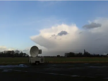
3.1 The NCAS mobile radar . . . 34

3.2 Location of Davidstow airfield . . . 35

3.3 Scan pattern coverage forCOPE10volume . . . 36

3.4 Location of Burn airfield . . . 41

3.5 Location of UKMO C-band radars . . . 42

3.6 Location of EA rain gauges . . . 43

4.1 Intermediate frequency drift during radar warm up . . . 46

4.2 Position of the radar during COPE campaign . . . 47

4.3 Raw reflectivity echo occurrence during the COPE campaign . . . 48

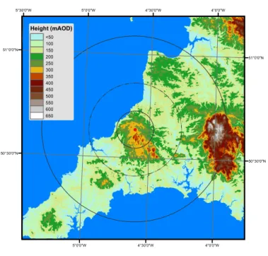
4.4 Surface elevation surrounding Davidstow . . . 49

4.5 Azimuthally averaged echo occurrence at increasing elevation angle . . . . 50

4.6 Raw reflectivity echo occurrence with threshold . . . 51

4.7 Conditional average reflectivity echo for the COPE campaign . . . 52

4.8 Radar filtered reflectivity - ground clutter example . . . 53

4.9 Radar filtered reflectivity echo occurrence compared to raw reflectivity . . 54

4.10 Radar filtered reflectivity - zero velocity example . . . 55

5.1 Histogram of horizontal radar reflectivity during rainfall . . . 59

5.2 Histograms of dual polarisation moments in rainfall . . . 60

5.3 Schematic representation of second trip echoes . . . 62

5.4 Example of second trip echoes . . . 63

5.5 UK radar composite, 2013-08-17 08:15 . . . 64

5.6 Dual polarisation moments for a second trip echo . . . 65

5.7 Dual polarisation moment histograms for second trip echoes . . . 66

5.8 Mean value SQI histograms for rainfall compared to second trip echoes . . 67

5.9 Median difference value histograms for rainfall compared to second trip echoes . . . 69

5.10 Two moment distribution heatmap for rainfall and second trip echoes . . 70

5.11 Variation in echo occurrence following second trip echo filtering . . . 71 xiii

(14)

5.12 Filtering error due to turbulent atmosphere . . . 72

5.13 Echo occurrence percentage after second trip echo filtering . . . 73

5.14 Variation of texture fields due to change of window shape . . . 79

5.15 Range correction of texture parameters . . . 81

5.16 Texture field histograms for rainfall echoes . . . 82

5.17 Normalised kernel density estimates for echo classification. . . 84

5.18 Multiple vertex membership function schematic . . . 86

5.19 Fuzzy logic classification of insects and convection - results . . . 91

5.20 Fuzzy logic classification of insects and convection - dual polarisation pa-rameters . . . 92

5.21 Fuzzy logic classification of rainfall and ground clutter - results . . . 94

5.22 Echo occurrence percentage after non meteorological echo filtering . . . . 95

5.23 Azimuthal echo occurrence percentage after non meteorological echo filtering 96 5.24 Fuzzy logic classification of rainfall and ground clutter at Burn airfield . . 97

6.1 Observed and processed differential phase shift . . . 104

6.2 Weighted average smoothing applied to differential phase shift . . . 105

6.3 Linear correction of attenuation in stratiform rainfall . . . 107

6.4 Linear correction of attenuation in convective rainfall . . . 109

6.5 Automation of ZPHI limits in stratiform rainfall . . . 112

6.6 Automation of ZPHI limits in stratiform rainfall - uncertainty . . . 113

6.7 Application of ZPHI correction to stratiform rainfall - PPIs . . . 115

6.8 Application of ZPHI correction to stratiform rainfall - radial example . . . 116

6.9 Application of ZPHI correction to convective rainfall - radial example . . 117

6.10 Dual polarisation beam blockage methods at 0.5◦degree elevation . . . 121

6.11 Azimuthal beam blockage variation with changingα . . . 121

6.12 Dual polarisation beam blockage methods at 0.5◦degree elevation . . . 122

6.13 PBB correction maps from dual polarisation observations . . . 122

6.14 Examples of partial beam blockage correction - COPE . . . 124

7.1 Accumulation of rainfall intensities . . . 128

7.2 Total rainfall accumulation for COPE - 0.5◦elevation . . . 131

7.3 Total rainfall accumulation for COPE near the radar - 0.5◦elevation . . . 132

7.4 Radar vs rain gauge rainfall accumulations for COPE . . . 134

7.5 Total rainfall accumulation for COPE near the radar - 1.5◦elevation . . . 135

7.6 Corrected horizontal reflectivity - 2013-08-17 11:57:46 . . . 136

7.7 Rainfall accumulations at Wadebridge - 2013-08-17 . . . 137

7.8 Rainfall accumulations at Roadford and Mary Tavy - 2013-08-17 . . . 138

7.9 Micro rain radar vertical profile of rainfall rate - 2013-08-17 . . . 140

7.10 Quasi-vertical profile of reflectivity - 2013-08-17 . . . 141

7.11 Rainfall accumulations at Wadebridge corrected for VPR . . . 142

7.12 Rainfall estimation using R(Z,ZDR) in 2D parameter space . . . 144

7.13 Rainfall estimates following linear correction of attenuation in convective rainfall . . . 146

7.14 Total rainfall accumulation for COPE - R(Z,ZDR) - 0.5◦elevation . . . 147

7.15 Radar vs rain gauge rainfall accumulations using R(Z,ZDR) for COPE . . 148

(15)

List of Figures xv

7.17 Rainfall estimates from KDP in convective rainfall . . . 152

7.18 Total rainfall accumulation for COPE - R(Ah) - 0.5◦elevation . . . 154

7.19 Radar vs rain gauge rainfall accumulations using R(Ah) for COPE . . . . 156

7.20 Rainfall using multiple dual polarisation estimators - decision tree . . . . 158

7.21 Weight functions for a weighted average dual polarisation rainfall estimate 159 7.22 Total rainfall accumulation for COPE Combined rainfall estimates -0.5◦elevation . . . 160

7.23 Radar vs rain gauge rainfall accumulations using combined rainfall esti-mates for COPE . . . 161

8.1 Schematic overview of the radar processing chain . . . 166

8.2 QVP from the RAINS field campaign - 2016-07-24 . . . 174

A.1 Location of EA Bealsmill river gauge . . . 182

(16)

(17)

List of Tables

2.1 Standard rainfall reflectivity conversion relations for differing atmospheric conditions and locations as presented in the literature . . . 8 2.2 The three most common weather radar frequency bands and their

respec-tive frequencies . . . 8 3.1 COPE radar operating periods . . . 37 3.2 Additional COPE instrumentation . . . 39 5.1 Radar parameters used in the classification scheme, as seen in Dufton and

Collier (2015). . . 78 5.2 Precipitation membership functions, reproduced from Dufton and Collier

(2015). . . 86 5.3 Ground clutter membership functions, reproduced from Dufton and Collier

(2015). . . 87 5.4 Noise membership functions, reproduced from Dufton and Collier (2015). 87 5.5 Insect membership functions, reproduced from Dufton and Collier (2015). 87 A.1 Location of EA rain gauges relative to mobile radar . . . 181

(18)

(19)

Symbols

A specific attenuation C radar calibration constant D drop diameter

G radar antenna gain

Kp / Kw dielectric factor of a particle (p) or water (w)

KDP specific differential phase

Ni drop number concentration

Pt transmitted power

¯

Pr mean received power

R instantaneous rainfall intensity Vt particle terminal fall velocity

Ze equivalent reflectivity factor

Zm measured reflectivity factor

ZDR differential reflectivity

a coefficient of standard rainfall rate equations b exponent of standard rainfall rate equations c speed of light in a vacuum

h,v subscripts denoting horizontal and vertical polarisation

r range of target

rmax maximum unambiguous range of the radar

t observation at time, t

α slope of linear relationship between specific attenuation and specific differential phase

(20)

β slope of linear relationship between specific differential attenuation and specific differential phase

δco backscatter differential phase between co-polar signals

δΦ median azimuthal phase difference

p / w complex index of refraction of the observed particle (p)

or water (w)

λ wavelength

ρco, ρhv co-polar correlation coefficient

ΨDP differential phase between co-polar signals

φDP forward propagation differential phase shift

between co-polar signals σ(...) texture of variable ...

θ1 3 dB beam width in the vertical plane φ1 3 dB beam width in the horizontal plane τ transmitted pulse width

(21)

Abbreviations

AP anomalous propagation

CASA engineering research centre for Collaborative Adaptive Sensing of the Atmosphere

CC correlation coefficient,ρco

COPE COnvective PrEcipitation experiment CPU central processing unit

DOP degree of polarisation DSD drop size distribution EA Environment Agency FIR finite impulse response GPU graphics processing unit

ICE-D Ice in Clouds Experiment - Dust IOP intensive observation period I/Q in phase and quadrature KDEs kernel density estimates LDR linear depolarisation ratio

MAPD Mean absolute percentage difference M d median

MPD Mean percentage difference MRR micro rain radar

NCAS National Centre for Atmospheric Science NCP normalised coherent power

NERC Natural Environment Research Council PPI plan position indicator

(22)

PRF pulse repetition frequency

QPE quantitative precipitation estimate QVP quasi-vertical profile

SEPA Scottish Environment Protection Agency SESAR Single European Sky ATM (Air Traffic

Management) Research SQI signal quality index UKMO UK Met Office

(23)

Chapter 1

Introduction

Flooding is a major challenge for many countries around the world, while drought can be equally devastating. Recent flash flooding has caused fatalities in Utah (Sep 2015), Macedonia (Aug 2015) and Morocco (Nov 2014), to name just a few examples, while the economic costs of larger flood events have been substantial, for example the 2007 summer floods in the United Kingdom cost more than £3.2 billion (Morris et al., 2010) and more recent flooding in Europe (2014) led to overe100 million of aid being distributed by the European Commission from the EU solidarity fund. Conversely the western USA, par-ticularly California has experienced an extended period of drought, with over 60% of the region being abnormally dry and at least 20% of the region suffering from severe drought or worse since the spring of 2012 and the UK was experiencing water deficit prior to the wet summer of 2012. Accurate measurements of rainfall allow the effective management of flooding situations, informing flood forecasts and providing context to events, while they also allow the evaluation of drought situations, improving understanding of their hydrological drivers. With the risk of flooding and drought predicted to increase over the coming century, as a result of increased population pressure, changes in land use and climate change (Conway et al., 2015; Veldkamp et al., 2015; Schneider et al., 2013; Kollat et al., 2012; Environment Agency and DEFRA, 2011), action to prevent, mitigate and manage these risks is required to lessen their future impacts. Rainfall measurements are just one aspect of this action, contributing to operational water resources planning and flood risk management, informing hydrological research as a critical input variable and also meteorological research, for assimilation into forecasts, forecast validation and

(24)

improved process understanding. The following thesis considers the use of weather radar for rainfall measurement, due to the continued expansion and technological development of weather radar networks across the world. Of particular importance is how the reliabil-ity of radar measurements may be improved for hydrological applications, and how the uncertainty of those measurements can be accurately represented.

1.1 Why use weather radar?

Weather radar provide distributed rainfall estimates at high spatial and temporal resolu-tion (1 km2 and 5 min for the current UKMO composite, for example), allowing rainfall to be estimated in real time across wide areas with a single instrument. As they observe the atmosphere at multiple elevation angles they can provide a more complete three dimen-sional view of the weather systems observed, allowing regions of interest to be studied in greater detail or short term extrapolations (nowcasts) to be made. The use of nowcasts is particularly relevant during periods of localised convective activity. In particular flash flooding from convective systems is a significant challenge for forecasters and flood risk management professionals (Moore et al., 2006; Collier, 2007; Broxton et al., 2014), and one which weather radar can help with. During convective situations it is common that the forecast location of individual cells is more uncertain than the forecast intensity, with current nowcasting systems using a distributed rainfall input from weather radar as an initial boundary condition to improve their performance, which is then advected to match modelled rainfall over the duration of the nowcast (Bowler et al., 2006; Golding, 2009; Hapuarachchi et al., 2011; Alfieri et al., 2012).

Another benefit of weather radar is the ability to produce distributed rainfall estimates. With the growing availability of distributed hydrological models facilitated by expanding CPU and GPU processing power the need to produce accurate measurements of dis-tributed rainfall as input has never been greater. The traditional hydrological input from rain gauges no longer meets these needs as rain gauge networks with a high enough spa-tial density for accurate distributed modelling are a rare occurrence and too costly to be implemented on an operational scale (Atencia et al., 2011).

Weather radars also provide the opportunity to measure additional atmospheric vari-ables, in addition to precipitation. Doppler technology allows the measurement of the

(25)

Chapter 1. Introduction 3

radial motion of the atmosphere in relation to the radar location, which can extended to absolute motion vectors provided overlapping radar coverage is available. Another newer technology, particularly in relation to the operational radar networks of Europe, includ-ing the network in the UK, is dual polarisation, which allows additional measurements of the shape and size of particles within the atmosphere.

Despite these advantages, and the long held view that weather radar are the next great development in hydro-meteorological observation for flood forecasting, the quantitative precipitation estimates obtained from weather radar are still not viewed as a reliable measurement. These estimates are often ignored in favour of simulated rainfall or inter-polated rain gauge data and when they are used they are heavily weighted to conform to rain gauge point measurements obtained at a vastly different temporal and spatial scale (Berne and Krajewski, 2013; Price et al., 2012; Neale, 2012). This approach can be attributed to the many uncertainties which affect quantitative precipitation estimates from radar (QPE) (Villarini and Krajewski, 2010a; Joss and Germann, 2000).

The aforementioned widespread implementation of dual polarisation weather radar sys-tems should change this perception, by improving the data quality and accuracy of radar QPE while better constraining the uncertainty in those measurements.

1.2 Assessing dual polarisation rainfall estimates

The following thesis will assess the magnitude of these improvements using a dual po-larisation radar dataset from the COnvective Precipitation Experiment (COPE) field campaign, obtained using a mobile, dual polarisation, Doppler X-band radar. To obtain accurate rainfall estimates the raw reflectivity dataset will be processed and corrected using multiple techniques made possible with dual polarisation observations, before con-trasting several methods of dual polarisation rainfall estimation to ascertain the uncer-tainty within the rainfall estimates. A final rainfall product for the field campaign will then be available which utilises these methods to provide the most accurate rainfall es-timate possible. The inclusion of multiple rainfall eses-timates from the radar in this final rainfall product will reduce its uncertainty through selective merging of the estimates, driven by the uncertainty analysis conducted throughout the thesis.

(26)

To achieve the above objectives it is first necessary to introduce rainfall estimation with weather radar, dual polarisation and the benefits of utilising dual polarisation (Chap-ter 2). Then the datasets used can be described in context (Chap(Chap-ter 3) and evaluated as an initial product (Chapter 4). Following initial analysis, which identifies common radar errors and uncertainties, the data can be quality controlled (Chapter 5) and cor-rected (Chapter 6) using dual polarisation techniques. Chapter 7 then introduces several methods of rainfall estimation using dual polarisation, comparing their output to rain gauges for the field campaign and describes the combination of these estimates into a final rainfall product for the COPE campaign.

(27)

Chapter 2

Introducing weather radar for

quantitative precipitation

estimation and hydrological

applications

The deployment of radar for meteorological observation began soon after its military development (Watson-Watt, 1945; Maynard, 1945). Despite these early beginnings its use for hydrological applications has always been secondary to other measurements of rainfall, especially rain gauges. Since this early inception two notable technological up-grades have occurred. The upgrade to Doppler systems, capable of measuring the radial velocity of detected echoes occurred in the 1980s and 1990s, with many countries across the globe now operating a multi-radar observational Doppler network (Meischner et al., 1997; Collier, 1996, for example). The second major technological improvement, dual polarization, has taken longer to reach operational networks, with networks such as the United Kingdom Met Office (UKMO) radar network and MeteoFrance’s radar network currently in the process of upgrade, and the United States WSR-88D network upgrade recently finished in 2013 (Figueras i Ventura et al., 2012; Zhu and Cluckie, 2012). These technological improvements aim to address many of the major sources of error in single polarisation radar measurements of rainfall, which are often cited as a major reason

(28)

for the continuing lack of confidence in radar data within the hydrological community (Villarini and Krajewski, 2010a; Neale, 2012). Another proposed solution to addressing these errors in radar QPE is the statistical modelling of the total combined errors when compared to a reference observation, typically rain gauges (Germann et al., 2009, for example). These error models can then be used to generate ensembles of rainfall fields which encompass the statistical variability of the radar errors.

Here follows an overview of single polarisation weather radar (2.1) and its uncertainties (2.2), dual polarisation radar (2.3) and how the application of dual polarization radar can address some of these uncertainties (2.4) and, finally the combination of radar obser-vations with rain gauge obserobser-vations which includes the development of observed rainfall ensembles (2.5).

2.1 Rainfall estimation with single polarisation weather radar

Single polarization radars transmit radiation in pulses, polarized along a known plane. These pulses then interact with the atmosphere and the hydrometeors within it, scattering the radiation. The radar then receives incoming radiation from this scattering, thereby observing the atmosphere. As hydrometeors are an incoherent radar target (Marshall and Hitschfeld, 1953) this received power is averaged over a number of pulses to produce the received signal. The number of pulses is determined by the scanning speed of the radar, the azimuthal gate spacing and the pulse repetition frequency. Once calculated the average received power (Pr) can then be converted into the equivalent radar reflectivity

factor (Ze) using the simplified radar range equation (2.1).

¯ Pr= C|Kp|2Ze(r0) r2 0 (2.1) Kp = 2_p−1 2 p+ 2 (2.2) C= PtG 2_θ 1φ1τ cπ3 λ2_{1024 ln(2)} (2.3)

In this case C is termed the radar calibration constant and is determined by the radar hardware configuration and pulse characteristics (see symbols section for components of

(29)

Chapter 2. Weather radar for hydrology 7

C) and should remain constant for a given radar, p is the complex index of refraction

of the observed particles and r0 is the range of the observed particles. See Collier (1996) or Bringi and Chandrasekar (2001) for full derivations of this formula, including a full treatment of the assumptions required. Equation 2.1 is valid when the observed particles are much smaller than the radar wavelength and Rayleigh scattering occurs, as is usually the case for weather radars. The other most pertinent assumptions are that the observed echo completely fills the radar beam volume and that a single p can be used to

char-acterise the observed particles, which is typically taken to be the di-electric constant of water (p), both of which can lead to errors in the retrieval ofZe, which will be covered

in the following section (2.2).

The advantage of converting radar received power to the equivalent reflectivity factor is that it can be directly related to the drop size distribution (DSD) of the observed volume, as first shown by Marshall et al. (1947). The relationship can be described as a function of the number of drops (Ni) of a given diameter (Di) and that diameter raised to the

sixth power, integrated over the whole range of diameters within the sample volume (Eq. 2.4).

Ze=

X

i

NiD6i (2.4)

For meteorological observations D can vary from≈50µm for cloud droplets to ≈8 mm for the largest raindrops and hail, leading to large variations in observedZe. As a result

it is typically expressed in units of decibels of reflectivity (dBZ) using a logarithmic transformation, as opposed to its linear units of mm6m−3. The reflectivity of a volume can then be related to rain rate (R) as the rain rate is also a function of the DSD. The relationship between diameter and rain rate (expressed in its common units of mm hr−1) is shown in equation 2.5. R= 0.6π×10−3 ∞ Z 0 N(D)D3Vt(D)δD (2.5)

where Ni is again the number of drops of a specified diameterDi andVt is the terminal

velocity of the drops, which is again a function of diameter. In practice a parametrised DSD is chosen for the climatological situation and then Eq. 2.4 and Eq. 2.5 can be

(30)

combined to allow calculation of rain rate using an equation of the form shown in Eq. 2.6.

Z =aRb (2.6)

In Eq. 2.6 the coefficient (a) and exponent (b) are dependant on the DSD parametrisa-tion used. Commonly used values are shown in table 2.1, though a wealth of different schemes have been derived for differing geographic locations and atmospheric conditions (for example Battan (1973) lists 60 different options developed across the world). The UK standard is to use a=200 and b=1.6 (Harrison et al., 2012).

Application a b

Drizzle 140 1.5 (Joss et al., 1970) Stratiform rain 200 1.6 (Marshall et al., 1955) Convective storm 500 1.5 (Joss et al., 1970) Met Office C-Band Radar 200 1.6 (Harrison et al., 2012) WSR-88D Radar 300 1.4 (Fulton et al., 1998) MeteoSwiss network 316 1.5 (Germann et al., 2006b)

Table 2.1: Standard rainfall reflectivity conversion relations for differing atmospheric conditions and locations as presented in the literature

It is also worth noting that across the world three distinct radar frequency bands, com-monly referred to as S-band, C-band and X-band, are used for rainfall estimation with weather radar (see Table 2.2 for details). This distinction is important when considering error sources for the radar system, the reasons why one may be chosen and also the potential benefits of dual polarisation to the system. In the United States the NEXRAD system uses high power S-band systems, in Europe C-band systems are more common (UK and Germany for example) and X-band is generally restricted to research systems (NCAS) and more recently urban scale radar coverage (CASA).

Band Frequency range (GHz) Wavelength (cm) Example system (wavelength) S 2 to 4 7.5 to 15 NEXRAD (10.7 cm) C 4 to 8 3.75 to 7.5 UKMO (5.4 cm) X 8 to 12 2.5 to 3.75 NCAS (3.2 cm)

Table 2.2: The three most common weather radar frequency bands and their respective

(31)

2.2 Error sources for single polarisation weather radar

The process of estimating rainfall using weather radar has many components which can be subject to error. Firstly there are errors in the process of measuring the received power, then in relating those measurements to the precipitation and finally in translating those precipitation estimates into rainfall accumulations at the ground. Each of these stages has several sources of uncertainty, which are covered in the following section, starting with processes which affect the measurement of the received power.

2.2.1 Radar calibration

The radar calibration constant (C, Eq. 2.3) is a clear source of error in the initial radar equation (Eq. 2.1) as it is a function of several hardware related variables, including the antenna gain, transmitted power, wavelength, the pulse dimensions and system losses. Due to the fluctuations in the radar components due to degradation and temperature fluctuations the true value of C can vary in time, with changes being difficult to detect from the radar data alone. Studies show that C can be calibrated to better than 1 dB (Collier, 1996) but this accuracy deteriorates with time from the calibration. For single polarisation radars detection is possible by comparison with other overlapping radar sites, giving a relative miscalibration between the two, through the use of a range of known reflectors (Atlas (2002) provides a good summary of target techniques) or by compari-son to other meteorological observations, such as rain gauge accumulations, disdrometer measurements and aircraft observations of drop sizes. Research by Manz et al. (2000) showed that the use of a target sphere provided the most accurate calibration (0.5 dB) for UK radars, provided that the sphere’s position could be accurately known and it be held stationary. Given the difficulty of these conditions, and the fact that a sphere could only be used for offline calibration they recommended an external transponder as the most accurate solution (still offline) or power monitor and test signal generator as the most feasible online calibration solution (quoted accuracy of 1.5 dB). An online solution allows more regular monitoring of the calibration and therefore more consistency in the measurements made, for example Germann et al. (2006b) indicate that weekly relative calibration is undertaken to ensure the stability of the MeteoSwiss radar network, while absolute calibration is not performed. Taking this approach allows for a stable set of

(32)

measurements which can then be bias corrected using long term observations to account for the lack of absolute calibration.

While miscalibration can be managed for single polarisation radars it can become a more serious issue when correcting for attenuation, where results can be extremely sensitive to calibration errors due to the cumulative effect of bias in the reflectivity measurements (Nicol and Austin, 2003; Hitschfeld and Bordan, 1954, for example). Attenuation will be explored further in the next section.

2.2.2 Attenuation

A reduction in received power can be caused by attenuation, where the beam power is reduced by hydrometeors between the radar and the target range. This causes the measured power (reflectivity, Zm) at a given range to no longer be directly comparable

to the reflectivity resulting from the observed rainfall DSD (Eq. 2.4, Ze), but instead

being a function of the true reflectivity and the intervening hydrometeors. The effects of attenuation were first detailed by Atlas and Banks (1951) for wavelengths shorter than 7 cm (C-band and X-band, for example) with long wavelength radars being unaf-fected by all but the most extreme rainfall events. This is a function of the relative size difference between the hydrometeors and the radar wavelength, and it is even possible for attenuation to cause complete extinction of the radar beam, such that observations beyond an attenuating storm cannot be made. Several studies have calculated the ex-pected attenuation due to differing phases of hydrometeors, changing temperature ranges and operating wavelengths (Delrieu et al., 1991; Wexler and Atlas, 1963; Gunn and East, 1954). For example, Delrieu et al. (1991) showed that at X-band attenuation ranged from about 0.1 dB km−1 _{for moderate rainfall intensities (8 mm hr}−1_{) to up to 3 dB km}−1 _for heavy rainfall (100 mm hr−1), with temperature variation only becoming significant at rainfall intensities in excess of 40 mm hr−1. C-band radars occupy a middle ground, with more moderate attenuation for a given rainfall (0.7 dB km−1 from a rainfall intensity of 100 mm hr−1) and a reduced temperature dependence at higher rainfall intensities. Clearly attenuation can cause serious changes in measured reflectivity, especially at short wavelengths, which reduces the accuracy of rainfall estimates when heavily precipitating storms are present.

(33)

To account for attenuation, many correction schemes have been developed (Nicol and Austin, 2003; Delrieu et al., 1997; Hildebrand, 1978; Hitschfeld and Bordan, 1954, for example), which are based on an attempt to quantify the attenuation and then return the measured reflectivity to a true reflectivity using a variation of the simple formula shown here, whereA(r) is the specific attenuation in dB km−1.

Ze(r) =Zm(r) + 2 r

Z

0

A(r)ds (2.7)

As Nicol and Austin (2003) explain, single polarisation attenuation corrections largely rely on the corrected reflectivity measurements along a segment to determine the attenuation (A(r)) at the end of the segment using an empirical relationship of a similar form to the Z-R relationship (Eq. 2.6), and as such any calibration bias can quickly lead to unstable solutions as the bias accumulates along the radial. As a result attenuation correction relies on a measurable constraint to prevent these divergent solutions, whether these be a power from a ‘known’ source such as a mountain (Serrar et al., 2000; Delrieu et al., 1999) or the use of external measurements such as rain gauges for a complete bias adjustment (Hildebrand, 1978). Even when these are available, errors persist in correction due to inherent variability in these measures and attenuation remains a significant problem for single polarisation radars.

In addition to attenuation from the atmosphere it is also possible for attenuation to occur due to wetting of the radome (Bechini et al., 2010; Baeck and Smith, 1998). Collier (1996) details the unpublished results of Eccleston and Hill (1980), showing the reduction in observed rainfall to be up to 15 mm h−1 due to radome wetting at the Clee Hill radar in the UK. It is possible to reduce these impacts using careful design, such as hydrophobic materials, geometry and size, but as Kurri and Huuskonen (2008) show, all radomes will cause attenuation in wet conditions.

2.2.3 Beam blockage

Another factor influencing the measurement of reflectivity and its comparison to the true reflectivity is the presence of a blockage within the radar beam, such as a hill, trees, buildings and other infrastructure. As the standard radar equation assumes that

(34)

the entire beam samples the pulse volume at the given range, a blockage introduces a reduction in received power for observations beyond the blockage and therefore a bias in the measurements. Provided the amount of beam blockage can be calculated, using a method such as that of Gabella and Perona (1998), the bias can be corrected. Calculating the degree of blockage relies on simple geometric optics, but requires accurate measures of surface topography (which is possible), the location and shape of buildings (more difficult), the refractive state of the atmosphere and possibly the vegetative state of the land causing the blockage. Bech et al. (2003) showed that refractivity changes in the atmosphere can change the bias caused by blockage by several dB, and as such static corrections cannot correct for all situations and are prone to errors in anomalous conditions. Many approaches only consider correcting blockage provided the degree of blockage is not too great, for example MeteoSwiss correct beam blocked data if less than 87% of the beam is blocked (Germann et al., 2006b), while the WSR-88D setup in the USA and the UK Met Office correct all data where the beam is 50% blocked or less (Fulton et al., 1998; Harrison et al., 2009). Even in these cases blockage can reduce echoes to below the background noise level, and correction is unable to recover this data leading to under measurement. In these cases and those where total beam blockage occurs, data extrapolation from higher elevation scans or adjacent rays is required (Germann et al., 2006b; Gabella and Perona, 1998).

As data that undergoes beam blockage correction is less reliable than clear sight obser-vations, careful choice of radar site is the best means of ensuring good quality data, the use of a terrain model technique like the one developed by Gabella and Perona (1998) prior to radar placement is therefore advised. Another approach is to only use beam elevations that do not suffer from beam blockage, however these higher elevations are prone to errors caused by sampling higher in the atmosphere, especially at longer ranges.

2.2.4 Non meteorological echoes

Alongside the issue of obtaining accurate reflectivity measurements, it is vital to deter-mine whether those measurements are from hydrometeors or another, non-meteorological, target. Common non-meteorological targets include ground clutter (which includes to-pography, vegetation and man-made structures), sea clutter (reflections from the sea

(35)

surface), biological scatterers (birds and insects), interference (RLAN and other radars) and even clear air echoes (due to humidity changes in the atmosphere).

Identifying, and removing, these spurious echoes is possible using either static techniques for known clutter, signal-level correction of the return pulse (Torres and Zrnić, 1999; Nguyen et al., 2008) or dynamic filtering (Steiner and Smith, 2002). Static maps, usually developed over time with summary statistics, are reasonably successful at removing the effect of ground clutter (Harrison et al., 2014, 2000). However when anomalous propaga-tion (AP) increases the area of the returns, through refracpropaga-tion of the beam closer to the ground surface, or when the ground clutter signals are a result of moving vegetation or wind turbines these static techniques become ineffective. They also are unable to remove echoes from other, non-meteorological sources, particularly biological scatterers.

Dynamic systems that respond to the variation in ground clutter returns due to AP have been developed as a response to these issues. Signal level, spectral filtering of the raw I/Q data received by the radar is one approach to this problem (Doviak and Zrnić, 1984, e.g.), provided the radar has Doppler capability. By processing the data prior to the radar generating a reflectivity measurement from the received power, ground clutter returns, which have a near zero Doppler velocity and a narrow spectral width, can be removed. However this can lead to the removal of weather echoes which also have near zero radial velocity, for example aggressive filtering of the WSR-88D network can lead to up to 20% of meteorological echoes being lost (Serafin and Wilson, 2000). Even with less aggressive filtering reflectivity is still removed along the so-called zero velocity isodop (Hubbert et al., 2009). Doppler filtering schemes also fail to cope with other sources of spurious returns, due to these returns having a velocity component.

There have also been many schemes created which utilise a machine learning approach, such as fuzzy logic, Bayesian inference or a decision tree, which incorporate the reflectivity measurements themselves along with vertical changes in reflectivity, the extent of the reflectivity, the spatial variability of the reflectivity and even Doppler fields if available (Pamment and Conway, 1998; Berenguer et al., 2006; Cho et al., 2006; Steiner and Smith, 2002, for example). In all these cases the identification of other non-meteorological echoes is not considered, due to the difficulty of identification with a single polarisation radar and also the fact that ground clutter / AP returns are the most significant non-meteorological source in terms of returned intensity and frequency of observation.

(36)

2.2.5 Parametrising the drop size distribution

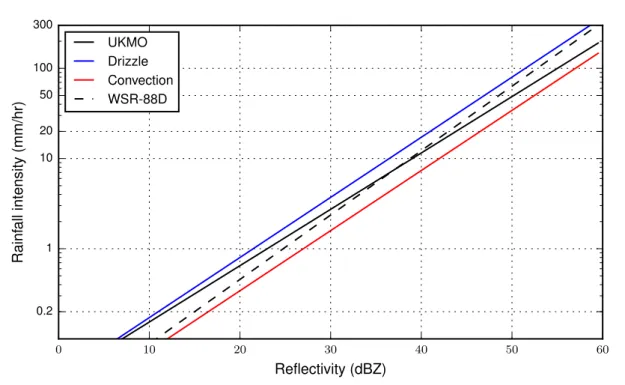
As already mentioned, there are a multitude of different possible parametrisations of the drop size distribution available, which determine the values of a and b in the ex-ponential rainfall-reflectivity relationship (Eq. 2.6). The wide range of available values describe differing precipitation processes, from tropical warm rain events which contain larger numbers of smaller drops (Fujiwara, 1967) to intense convective systems where the distribution has a much greater median diameter (Joss et al., 1970). Even within these classically defined precipitation types there is a great variation in the values presented with this variability all inherent within one possible radar scan which leads to uncertainty in the ’best’ value to use for a given observation (Atlas et al., 1999; Uijlenhoet et al., 2003). Figure 2.1 shows just a small subset of the available parametrisations and high-lights the possible variation in retrieved rainfall depending on the DSD parametrisation chosen, for example just using the four distributions shown a reflectivity measurement of 40 dBZ could equate to a rainfall intensity of between 8 and 20 mm hr−1depending on the type of rainfall being observed. In order to deal with DSD variations, pre-classification of echoes is required to allow the application of an appropriate parametrisation, particu-larly in the USA where the radar network covers an extensive geographical area with wide variations in atmospheric conditions. For single polarisation radar this is achieved using the intensity of the reflectivity measurements, generally in combination with their three dimensional structure(Rosenfeld et al., 1995; Steiner et al., 1995; Anagnostou, 2004; Qi et al., 2013), with results showing improved rainfall estimation provided the classification can be achieved with a high level of accuracy.

2.2.6 Variations in hydrometeor phase

One of the main limitations of the assumptions is that the particles must be considered to be all of the same phase (water or ice), not a mixture. In practice this leads to K (Eq. 2.2) for water being used as standard and an overestimation of Zm when solid

hydrometeors are observed. To counteract this DSD parametrisations for snow and ice exist, and can be applied provided it is possible to identify solid phase hydrometeors. The presence of both solid and liquid phase precipitation intermixed within a sample volume presents an even greater challenge and single polarisation radars struggle to make accurate

(37)

Chapter 2. Weather radar for hydrology 15 0 10 20 30 40 50 60 Reflectivity (dBZ) 0.2 1 10 20 50 100 300 Rainf all intensity (mm/hr) UKMO Drizzle Convection WSR-88D

Figure 2.1: Variation in retrieved rainfall intensity resulting from the use of different DSD parametrisations. The four shown are taken from Table 2.1.

precipitation estimates in these cases. Another consequence of changes in hydrometeor phase is the impact on attenuation corrections, as mixed phase particles can have a stronger attenuating affect than purely liquid phase particles, with solid cores supporting large liquid drops (Ryzhkov and Zrnić, 1995), while ice crystals have a much smaller attenuating affect than liquid precipitation (Vivekanandan et al., 1994).

The most documented example of hydrometeor phase causing rainfall estimation errors is in the case of the bright band, which is elevated reflectivity due to the radar beam intersecting the melting layer in stratiform conditions (Austin and Bemis, 1950; Hooper and Kippax, 1950; Klaassen, 1988; Huggel et al., 1996; Sánchez-Diezma et al., 2000, for example). The strength of the enhancement is dependent on the elevation angle and the range at which the beam intercepts the melting layer, along with the fall speed of the melting hydrometeors. The regions of enhanced reflectivity can generally be identified using a combination of the radar data and information about the melting layer height (from numerical models or radiosondes for example) and then corrected for using a vertical reflectivity profile to transform elevated reflectivities to their surface equivalent (Smith,

(38)

0 10 20 30 40 50 60 Reflectivity (dBZ) 0.2 1 10 20 50 100 300 Rainf all intensity (mm/hr) GM 1958 C 1968 SS 1970 UKMO - rain

Figure 2.2: Variation in retrieved precipitation intensity resulting from the use of different DSD parametrisations for snowfall. The relations shown are from Gunn and Marshall (1958), Carlson (1968) and Sekhon and Srivastava (1970) respectively. The

UKMO rainfall parametrisation is shown for comparison.

1986; Kitchen et al., 1994; Hardaker et al., 1995; Smyth and Illingworth, 1998b; Gourley and Calvert, 2003; Rico-Ramirez and Cluckie, 2007).

2.2.7 Rainfall accumulation

An inherent aspect of radar QPE is that the radar observes instantaneous rainfall in-tensity in specific volumes of the atmosphere, while hydrological applications generally use surface rainfall accumulations in a given time period over a defined area, be it a river catchment or a model grid box (Beven, 2011). Jordan et al. (2000) found that the largest contribution to this uncertainty is the fact that the radar measures at a given height above the ground, with the random variability increasing with height and reduc-ing given the size of the accumulation area. Clearly usreduc-ing radar observations from as close to the ground as possible provides the most representative measurements, but this must be balanced against the increased likelihood of partial beam blockage and ground clutter returns as discussed above. Another uncertainty in converting rainfall intensities

(39)

of rainfall to accumulations is the temporal variability of the rainfall over the accumula-tion interval, and the number of radar observaaccumula-tions that fill that sampling volume. For example, Wilson and Brandes (1979) show that the greater the sampling interval the larger the variability in the comparison between radar and rain gauges, while Villarini et al. (2008) show that the variability is largest over the shortest accumulation intervals given a fixed measurement interval. To reduce the uncertainty from a radar perspec-tive it is important to have as short as possible interval between measurements, while schemes have also been developed which interpolate between observations to generate more accurate accumulations (Liu and Krajewski, 1996; Tabary, 2007, for example).

2.3 Dual polarisation weather radar

The first application of dual polarisation to weather radar was by Seliga and Bringi (1976) but it is only in the past decade that dual polarisation radars have been incorporated into national observational networks such as the United States of America’s NEXRAD / WSR-88D programme (upgrade completed in summer 2013) and the United Kingdom Met Office’s radar network (upgrade ongoing, completion expected in 2018).

As opposed to single polarisation radar, dual polarisation radars transmit and receive along two planes of incidence, typically the horizontal and vertical planes (Fig. 2.3). The addition of a second plane of observation allows comparative radar moments to be studied, which investigate the relative changes between the two planes. These moments include the differential reflectivity, the differential phase shift and the co-polar cross correlation, among others, which are discussed in section 2.3.2. Prior to the discussion of these new moments it is necessary to differentiate between the two possible implementations of dual polarisation available, as they can provide different moments and levels of accuracy.

2.3.1 Simultaneous vs alternating transmission

There are several possible transmission and reception modes for dual polarisation radars determined by the configuration of the radar hardware, particularly the number of re-ceivers and the presence of a waveguide switch. The two main modes of operation are alternating transmission, with dual receivers and simultaneous transmission with dual

(40)

Figure 2.3: Two orthogonal polarised planes in the horizontal (solid) and vertical (dashed). Transmitted in the direction of the arrow, with zero phase offset.

receivers (Bringi and Chandrasekar, 2001). In alternating transmission mode the state of the transmitted pulse is switched alternately between the horizontal and vertical state (hv), although some systems implement a repeated block pulsing of these states such as

hhv orhhvv(Fig. 2.4). This allows sampling of the cross-polar elements of the scattering matrix, while co-polar elements are only available where that state is transmitted (every other pulse for the simple alternating state). In simultaneous or hybrid transmission mode both planes are transmitted at the same time, with the received orthogonal signals being a combination of the copolar and cross polar return signals from the transmitted wave (Fig. 2.4).

The advantages of alternating transmission mode, or a block pulse style derivative, are that the linear depolarisation ratio (LDR) can be measured, that measurement errors are less sensitive to antenna polarisation errors and that the system isolation require-ments are lower for a specific required observational accuracy (Wang and Chandrasekar, 2006). Conversely the advantages of hybrid transmission are direct measurement of the coherency matrix, leading to direct estimation of both the copolar correlation coefficient and the propagation phase (with greater unambiguous range), more accurate variables for

(41)

a given scan rate due to twice the number of observations and lower cost radar hardware as a waveguide switch is not required (Doviak et al., 2000).

H V H V H V A H H V H H V B H V H V H V C

Figure 2.4: Schematic pulse diagrams of alternating (A), block pulsed hhv (B), and simultaneous (C) transmission.

2.3.2 Dual polarisation moments

As already mentioned, the addition of a second, orthogonal, plane of transmission to weather radars allows the measurement and estimation of several new radar moments based on differences between the two planes. These new moments provide additional information about the echoes being sampled, which are of great use in radar hydrome-teorology. These new parameters are the differential reflectivity (ZDR), the differential

phase shift (ΨDP) (which is composed of the forward propagation phase shift (ΦDP) and

the backscatter differential phase shift (δco)), the specific differential phase (KDP), the

co-polar cross correlation (ρco) and the linear depolarisation ratio (LDR). The

follow-ing section describes each of these parameters in turn, along with a description of their physical meaning. The benefits of these new moments are then covered in the following section (2.4)

(42)

2.3.2.1 Differential reflectivity

Differential reflectivity (Z_DR) is the observed ratio of the horizontally and vertically polarized linear reflectivity measurements. It was first proposed as a method of ob-serving rainfall by Seliga and Bringi (1976), with the aim being to add information to help quantify the rainfall drop size distribution. Due to the oblate spheroidal shape of falling raindrops, they produce a positive reflectivity shift in the horizontal, relative to the vertical, which is proportional to their diameter. Scattering simulations and field measurements show that Z_DR ranges from 0.2 dB in very light drizzle to over 4.5 dB for very large rain drops (Seliga and Bringi, 1978; Hall et al., 1984; Balakrishnan and Zrnić, 1990, for example). Scattering simulations by Ryzhkov and Zrnić (2005) quantified this relationship for S, C and X-band wavelengths and show the variation between them, with X-band suffering from minor resonance effects at a diameter of 3.5 mm and C-band suffering from more extreme resonance effects at diameters above 5 mm (Fig. 2.5). These resonance effects are the result of Mie scattering (Matrosov et al., 2002; Meischner et al., 1991), with the reduced resonance at X-band believed to be a consequence of increased absorption dampening the resonance effect (Park et al., 2005; Ryzhkov and Zrnić, 2005).

0 1 2 3 4 5 6 7 8 Equivolume diameter (mm) 0 1 2 3 4 5 6 7 8 ZD R (d B ) X-band S-band C-band

Figure 2.5: Theoretical variation of differential reflectivity with increasing equivolume

(43)

2.3.2.2 Differential phase shift

The total differential phase shift (Ψ_DP) is the observed phase difference between the received horizontal and vertical pulses and contains two components, the backscatter differential phase (δco) and the propagation differential phase ΦDP (Eq. 2.8) (Bringi and

Chandrasekar, 2001). As there is often a phase shift on transmission the received phase shift also contains this component, which must be removed to gain the shift resulting from atmospheric interaction.

ΨDP = ΦDP +δco (2.8)

The differential propagation phase measures the change in phase between the horizontal and vertical phase of returns along the beam path which varies as a function of the total cross section of scatterers along the path. Therefore it varies as a function of both axis ratio of the drops and number of drops, with measurements in rainfall monotonically increasing along the beam path due to the positive axis ratio of raindrops (Seliga and Bringi, 1978; Jameson, 1985). Due to this dependence on the DSD, phase shift has frequently been proposed as an additional means of estimating rainfall using weather radar (Sachidananda and Zrnic, 1986, for example). These approaches have often been limited to higher rainfall rates as the phase shift is inversely proportional to wavelength for a given rainfall rate, with most early studies using S-band systems (Matrosov et al., 1999). Conversely the phase shift for an X-band system is 3 times greater than at S-band, which increases the sensitivity to lower rainfall rates. As a cumulative quantity the propagation phase is often differentiated with range to calculate the specific differential phase (KDP) for each range gate for the purposes of rainfall estimation (see next section).

The backscatter differential phase forms the second component of the observed phase difference (Eq. 2.8). It is a function of non-Rayleigh scattering and is not cumulative along the rain path but a function of the distribution of scatterers in each range gate. Due to it being a function of non-Rayleigh scattering it is often ignored at S-band, but becomes an increasing component of the measurements at lower wavelengths, particularly X-band when equivolume drop diameters exceed 2 mm (Matrosov et al., 1999). As the backscatter phase has often proven difficult to separate from the total phase difference

(44)

measurements its use has been limited, however recent studies including Trömel et al. (2013) and Tyynelä et al. (2014) have begun to explore the potential of using backscatter differential phase, particularly for observing melting particles.

2.3.2.3 Specific differential phase

The specific differential phase (KDP) is simply the range derivative of the forward

prop-agation differential phase Φ_DP, typically expressed in units of degrees per kilometre (◦ km−1). It is a calculated, rather than measured, radar moment, being derived from one component of the measured differential phase shift. At shorter wavelengths calcu-lation requires either the filtering of the observed phase shift to remove the backscatter component, or careful selection of the calculation path to ensure the change in backscat-ter between the start and end of the path is minimal. The simplest method of calculation is a finite difference along a range path, however for rainfall estimation a more accurate method is required (Bringi and Chandrasekar, 2001). These methods include linear re-gression over varying path lengths (Ryzhkov and Zrnic, 1996), iterative range smoothing (Hubbert and Bringi, 1995), solving linear equations with linear programming (Gian-grande et al., 2013) and even calculation using the angular domain with cubic spline estimation of KDP (Wang and Chandrasekar, 2009).

2.3.2.4 Co-polar cross correlation

The co-polar cross correlation coefficient (ρco) is the correlation between the co-polar

return at horizontal polarisation and the co-polar return at vertical polarisation. For alternating transmission mode only one of the co-polar elements can be measured per pulse and the co-polar correlation has to be estimated given the time lag between pulses. For simultaneous transmission the cross-polar components of the received powers are negligible compared to the co-polar components of the powers and therefore the co-polar cross correlation can be taken to be the measured co-polar correlation. However, in the presence of cross-polarizing scatterers, the measured value begins to deviate from its intended physical description as detailed by Galletti and Zrnić (2012). By measuring the correlation between the two pulses the homogeneity of the sample volume can be assessed, for example raindrops exhibit a large degree of spatial homogeneity and therefore have

(45)

correlations above approximately 0.97 (Balakrishnan and Zrnić, 1990). Mixed phase returns, particularly the melting layer have lower correlations, typically reported to be around 0.9 (Ryzhkov et al., 2005b; Bringi et al., 1991; Balakrishnan and Zrnić, 1990), although this is somewhat dependant on the radar configuration (particularly the dwell time and the beamwidth), for example Illingworth and Caylor (1989) observed values as low as 0.6 in the bright band with a 0.25 degree beamwidth S-band radar, while Zrnić et al. (2006) showed the variation of correlation with antenna rotation speed, with faster speeds leading to lower expected values. As a result the co-polar cross correlation is a useful parameter for identifying mixed phase returns, and also for identifying regions of non-meteorological echoes (see 2.4.1).

2.3.2.5 Linear depolarisation ratio

The linear depolarisation ratio is the amount of depolarisation which occurs due to cross polarising scatterers. To measure LDR requires the radar to operate in alternating trans-mission mode, such that a single polarisation is transmitted at any one time, and that both received polarisations are recorded. The LDR is then the amount of signal that is converted from the transmitted orientation (either horizontal or vertical) to the or-thogonal direction by the observed hydrometeors. LDR increases with rainfall intensity as heavier rainfall has a more varied DSD, but is greater still for melting snow, hail, and strongly orientated ice crystals which all exhibit more variability in their shape and movement during descent (Bringi et al., 1986; Brandes and Ikeda, 2004; Ryzhkov and Zrnic, 2007). As such LDR is most often used in identification of scatterers, particularly solid phase scatterers.

2.4 Applications to hydrometeorology

There are three main applications of dual polarisation moments which can lead to im-provements in rainfall estimates from weather radar. The first is the use of dual polar-isation for quality control of the incoming data (2.4.1), filtering out non-meteorological echoes and highlighting areas of degraded signal quality due to attenuation and/or beam blockage. This prevents spurious echoes being converted into rain rate and highlights ar-eas where interpolation or adjustment may be required to improve the data quality. The