Empirical Analysis ot the Top 800 Cryptocurrencies using Machine Learning Techniques

(1)

Empirical Analysis ot the Top 800

Cryptocurrencies using Machine Learning

Techniques

Teresa Riedl

A dissertation submitted to the Faculty of Commerce, University of Cape Town, in partial fulfilment of the requirements for the degree of Master of Philosophy.

January 9, 2019

MPhil in Mathematical Finance, University of Cape Town.

University

of

Cape

(2)

The copyright of this thesis vests in the author. No

quotation from it or information derived from it is to be

published without full acknowledgement of the source.

The thesis is to be used for private study or

non-commercial research purposes only.

Published by the University of Cape Town (UCT) in terms

of the non-exclusive license granted to UCT by the author.

University

of

Cape

(3)

Declaration

I declare that this dissertation is my own, unaided work. It is being submitted for the Degree of Master of Philosophy to the University of Cape Town. It has not before been submitted for any degree or examination.

Teresa Riedl

(4)

Abstract

The International Token Classification (ITC) Framework by the Blockchain Center in Frankfurt classifies 795 cryptocurrency tokens based on their economic, tech-nological, legal and industry categorization. This work analyzes cryptocurrency data to evaluate the categorization with real-world market data. The feature space includes price, volume and market capitalization data. Additional metrics such as the moving average and the relative strengh index are added to get a more in-depth understanding of market movements. The data set is used to build supervised and unsupervised machine learning models. The prediction accuracies varied amongst labels and all remained below 90%. The technological label had the highest pre-diction accuracy at 88.9% using Random Forests. The economic label could be predicted with an accuracy of 81.7% using K-Nearest Neighbors. The classifica-tion using machine learning techniques is not yet accurate enough to automate the classification process. But it can be improved by adding additional features. The unsupervised clustering shows that there are more layers to the data that can be added to the ITC. The additional categories are built upon a combination of to-ken mining, maximal supply, volume and market capitalization data. As a result we suggest that a data-driven extension of the categorization in to a token pro-file would allow investors and regulators to gain a deeper understanding of token performance, maturity and usage.

(5)

Acknowledgements

I would like to express my very great appreciation to Dr. Co-Pierre Georg for his guidance throughout the past year together with the AIFMRM team and especially Lameez and Lizzy. Thank you David for giving us exposure to your network and the supporters of AIFMRM. I would like to offer my special thanks to Luca Frag-nani and Philipp Sandner at the Blockchain Center in Frankfurt for providing the Token Classification and support in drawing the initial hypotheses. Although the data could not be used for the analysis, I would like to thank the Santiment team for their openness and willingness to collaborate. I could not have succeeded through-out this year withthrough-out Dustin being by my side. Thank you for the positivity through all the ups and downs, home-cooked meals, parkruns and morning swims. Pursu-ing this degree would not have been possible without the support of my family in Germany. Mum, dad thank you for always being there for me and letting me pursue my dreams and adventures. Nick Hops your help was greatly appreciated. And last but no least a great and most special thanks to my fellow students and especially Ashleigh, Jonjon, Bryony and Masego. You will all strive and change the world for the better. I cannot believe it is over!

(6)

List of Figures

1.1 Total Cryptocurrency Market Capitalization and Volume in USD . . 4

1.2 Dimensions of the International Token Categorization Framework. . 6

3.1 Exemplary time series element from CoinMarketCap . . . 13

3.2 Exemplary element of the token classification . . . 13

3.3 Ripple Time Series Decomposition . . . 16

3.4 Boxplot for Supply Circulation Feature. . . 20

3.5 Correlation Matrix Visualization for 34 Numeric Features . . . 21

3.6 Number of Tokens per Primary Label . . . 23

3.7 Number of Tokens per Primary Economic, Legal and Industry Label 24 3.8 Tech Labels in Relation to Token Mining . . . 25

3.9 Tech Labels in Relation to Maximum Supply . . . 25

4.1 Shrinkage Method XGBoost . . . 29

4.2 Cumulative Variance Explained for First Five Components . . . 31

4.3 2-D Principal Components for Primary Tech Labels . . . 31

4.4 KNN-Accuracy for XGBoost Feature Selection based on Number of Neighbors . . . 33

4.5 KNN-Confusion Matrix for XGBoost Feature Selection Test Set . . . . 34

4.6 Cost-Cluster Plot to Determine Optimal Number of K . . . 38

4.7 K-Means Scatterplot based on First Two Principal Components K=2 . 38 4.8 K-Means Scatterplot based on First Two Principal Components K=5 . 39 4.9 Hierarchical Clustering Dendrogram K=5 . . . 41

A.1 International Token Classification. . . 50

A.2 Token Classification Framework . . . 51

A.3 Functional Blockchain Crypto Property Classification. . . 52

B.1 Unscaled Data Boxplots . . . 53

B.2 Scaled Data Boxplots . . . 54

B.3 Log-Transformed Data Boxplots. . . 55

B.4 Number of Tokens per Secondary Labels Economic and Industry . . 56

B.5 Number of Tokens per Secondary Labels Tech and Legal . . . 57

C.1 Best Subset Selection Chi Squared Test Primary Economic Label . . . 58

C.2 XGBoost Feature Importance Primary Tech Label. . . 59

C.3 XGBoost Feature Importance Primary Legal Label . . . 60

(9)

C.5 2-D Principal Components Feature Directions. . . 62

C.6 2-D Principal Components for Primary Economic Labels . . . 63

C.7 2-D Principal Components for Primary Legal Labels . . . 63

C.8 2-D Principal Components for Primary Industry Labels . . . 64

D.1 Evaluation of Supervised Learning Techniques for Classification by Kotsiantiset al.(2007) . . . 65

E.1 Hierarchical Clustering Dendrogram K=2 . . . 67

E.2 Complete Hierarchical Clustering Dendrogram K=5 . . . 68

E.3 Hierarchical Clustering Scatterplot based on First Two Principal Com-ponents K=2 . . . 69

E.4 Hierarchical Clustering Scatterplot based on First Two Principal Com-ponents K=5 . . . 69

(10)

List of Tables

3.1 Table of Metrics with Missing Values . . . 18

3.2 Table of Metrics with Missing Values . . . 19

3.3 Non-zero, positive features for Log-Transformation . . . 20

3.4 No-claim Investment Tokens . . . 24

4.1 Selected Feature Selection Techniques . . . 28

4.2 XGBoost Maximal Accuracies and Optimal Number of Features for Primary Labels . . . 29

4.3 Economic Label Prediction Accuracies based on Model Feature Se-lection . . . 36

4.4 Tech Label Prediction Accuracies based on Model Feature Selection. 37 4.5 K-Means Clustering Overview for K=5. . . 40

4.6 Hierarchical Clustering Overview Token Mining and Max Supply for K=5 . . . 41

4.7 Hierarchical Clustering Market Metrics for K=5. . . 42

D.1 Legal Label Prediction Accuracies based on Model Feature Selection 66 D.2 Industry Label Prediction Accuracies based on Model Feature Selec-tion . . . 66

(11)

Chapter 1 Introduction

”Ten years after the invention of Bitcoin it is indisputable: Blockchain Technology will revolutionize the finance sector. In order to be part of its success, Germany has to act now.”

Handelsblatt, November 1, 2018

Regulators have fallen behind in creating a fruitful environment for cryptocurrency companies. Certainly, for the right reasons: to protect investors, to let the technol-ogy evolve and to understand the impact blockchain technoltechnol-ogy can have on the state, the financial system and the population. The cryptocurrency community is becoming impatient and regulators are seeking to provide the right balance be-tween freedom and regulation.

Throughout the cryptocurrency hype in 2017 the new field became a hot topic in research and analysis. Scientists were battling with each other to build the best price prediction models and to estimate the future of the market. Although few people knew what one was talking about in early 2017 when mentioning Bitcoin -at the end of the year the topic was on everyone’s lips. Yet the convers-ation was less about the technology, its vision and drawbacks than about the price, the possi-ble value a few months from now and the potential returns people could make. After the decline of the market in early 2018, the conversations seem to have van-ished, except for a few comments about whether the value will drop to zero or not. There are ambitious entrepreneurs out there who believe in the technology and are seeking to build sustainable businesses. For them the calmness might in some cases be a relief and an opportunity to focus on the core: getting the basics right and un-derstanding cryptocurrencies, their risks and values.

This work conducts an exploratory analysis of the top 795 cryptocurrencies1 us-ing data analytics tools and machine learnus-ing techniques. One valuable step in the

(12)

1.1 Blockchain Technology and Cryptocurrency Tokens 2

process of regulation and risk assessment is the classification of cryptocurrency to-kens. In this research the empirical analysis of cryptocurrency market data is put into relation with the token classes: economic purpose, technological setup, legal claim and industry.

The following section will give a brief overview of blockchain technology and the cryptocurrency market with focus on the past two years. It then goes on to outline the Token Classification Framework to understand the basis of this work.

Thereafter, chapter 2 describes related work that has been done in the new research field of Blockchain Technology and especially on Cryptocurrency Tokens. Chapter 3 outlines an exploratory analysis of the cryptocurrency market with regards to correlations amongst tokens and insights that one can gain per token. Chapter 4 will explore the token classification done by the blockchain center with regards to numberic characteristics of the tokens. In Chapter 5 the findings are discussed and an outlook is provided.

1.1 Blockchain Technology and Cryptocurrency Tokens

The focus of this section is to provide a non-technical introduction into Blockchain Technology and Cryptocurrency Tokens.

In 2008 the Bitcoin Whitepaper, published under the acronym ”Satoshi Nakamoto”. Nakamoto(2008) proposed a system for electronic (cash) transactions without rely-ing on trust. As opposed to existrely-ing systems such as SEPA or Paypal transactions, Satoshi suggested a peer-to-peer system that allows ”online payments to be sent directly from one party to another without going through a financial institution” (Nakamoto,2008).

Satoshi’s proposal can be broken down into three elements: the system, electronic cash and trustless peer-to-peer transactions. The ”system” is the underlying block-chain technology platform. It is used as a database to store a ledger of all transac-tions. Unlike databases used in banks and other institutions, the database is public and decentralized. Decentralized means that individuals around the world store a copy of the database (Swan, 2015, chap. 1). Examples for blockchain technology platforms are Bitcoin and Ethereum. ”Electronic cash” is the mean of exchange on the blockchain technology platform and widely known as cryptocurrency, coin or token. Cryptocurrencies are different from fiat currencies as they are not issued

(13)

1.1 Blockchain Technology and Cryptocurrency Tokens 3

by central banks but by the companies who developed the underlying protocols. They are seen as privately issued currencies. The protocol is the third element. By implementing logic and incentive structures via code, protocols create trust envi-ronments for peers (Swan,2015, chap. 1). The peer-to-peer transaction of value is one use case that a protocol can fulfill. Some other applications for blockchain pro-tocols are transactions of financial assets such as stocks or private equity, land or property registries and identification of individuals by issuing passports or licenses on the blockchain technology platform.

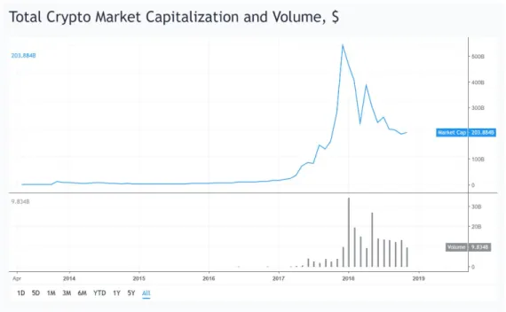
Since the Bitcoin Whitepaper was published it took nearly five years for Bitcoin to be launched as the first cryptocurrency. Today (Nov 2018) there are more than 2000 cryptocurrencies listed on CoinMarketCap2. In 2017 the number of cryptocurren-cies increased exponentially and so did the cryptocurrency market capitalization overall as figure1.1indicates3. In December 2017 the market reached its peak and thereafter fell back to less than half of the maximum market capitalization4.

The development of the cryptocurrency market suggests a comparison with the Gartner Hype Cycle although it is not safe to say whether the negative hype has already reached its minimum. It is likely that the slope of enlightment (Linden and Fenn,2003) will arrive eventually. For the market to mature the environment has to provide the necessary regulations to make it safe for entrepreneurs and investors to place their resources. As the technology is still new and constantly evolving regula-tors are taking various routes. Small countries such as Singapore and Gibraltar are at the forefront allowing blockchain companies to operate and issue licenses. Their main motivation is attracting new businesses and thereby tax income. In addition the volume of new companies registering is still manageable. Large countries are often more hesitant - not to say rigorous. China for instance banned all initial coin offerings (ICO) and cryptocurrency-to-fiat exchanges in September 20175. How-ever, China favours innovation and is at the same time experimenting with a state issued cryptocurrency in order to remain in control of funds flowing and in and out of the country. In England and South Africa regulators allow ”sandbox projects” to operate under supervision of regulatory authorities. Thereby regulators assure 2_{https://coinmarketcap.com/ CoinMarketCap is a website that tracks cryptocurrency data. Each} currency is listed with its real-time price (averaged across exchanges) and related data such as market capitalization and trading volumes.

3_{https://www.tradingview.com}

4_{The cryptocurrency market capitalization is calculated by multiplying the price by the number of} tokens in circulation. This calculation is controversial as the price decreases instantly with a decrease in demand.

(14)

1.2 International Token Classification Framework 4

Fig. 1.1:Total Cryptocurrency Market Capitalization and Volume in USD that new businesses operate within the countries laws and at the same time they learn to regulate companies with similar operations.

With the sheer volume of new companies entering the market since 2017, the need for measures to categorize and differentiate blockchain companies, to evaluate their risk and to define their legal status increases drastically together with the need to understand the market as a whole. As a starting point the Blockchain Center at the Frankfurt School of Management developed a cryptocurrency token classifica-tion framework. It is meant to serve as a foundaclassifica-tion for blockchain regulaclassifica-tion and taxation globally.

1.2 International Token Classification Framework

This section gives an overview of the token classification framework that has been developed by the Blockchain Center (BC) at the Frankfurt School of Management in Germany.

In the previous section we stated that a cryptocurrency is a privately issued cur-rency (Mougayar, 2016, chap. 1). In this paper cryptocurrencies will be widely referred to as tokens.

(15)

In 2017 the Frankfurt School of Finance & Management in Germany launched a think tank and research center for blockchain technologies and emerging busi-nesses. The Blockchain Center’s intention is to be a knowledge platform for indus-try experts, start-ups and corporates6. Since its initiation, the Blockchain Center published research papers on blockchain technology in various contexts such as chemical industry, mobility, internet of things, sharing economy and manufactur-ing. In addition, the team performes due diligence on existing blockchains such as Ethereum. Through their research, webinars and conferences, the Blockchain Cen-ter has become a widely renowned institution in Europe and works closely with the German Federal Financial Supervisory Authority (BaFin7).

The motivation behind the International Token Classification (ITC) Framework is to provide a ”tangible and holistic framework for the identification, classification and analysis of different token types”8. The framework is a starting point for regulators and tax authorities to consistently assess the legal and tax implications, associated risks and investment suitability of tokens9.

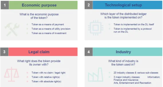
The proposed framework has been developed over the course of several months by continuously testing and extending the logic until the outcome was suitable to classify the 800 highest ranked tokens by market capitalization. The result is a multi-dimensional approach and consists of four levels: Economic Purpose, Tech-nological Setup, Legal Claim and Industry.

For a detailed description of the different layers of each category and their sub-categories appendixAoutlines all categories and definitions. The categorization caters for regulators, tax authorities, researchers and for investors who are seeking measures to evaluate risk and value of each token. Figure1.2indicates the basic sub-categories but the complete framework consists of a total of 70 categories and may be explored in more detail inA.1.

The economic purpose can be understood when considering certain examples. Bit-coin serves as an example for payment tokens as its primary use. Ethereum’s token Ether is used as a fee to use the Ethereum platform to build upon. Utility tokens are cryptocurrencies with a pre-defined use, in this case Ethereum owners can make use of the Ethereum infrastructure to deploy and execute smart contracts. The least

6_{https://www.frankfurt-school.de/home/research/centres/blockchain} 7_{Bundesanstalt f ¨ur Finanzdienstleistungsaufsicht}

8_{Frankfurt School Blockchain Center Newsletter November 2018} 9_{https://www.mme.ch}

(16)

Fig. 1.2:Dimensions of the International Token Categorization Framework frequent economic category is investment (or security) tokens. ICONOMI is a dig-ital asset management platform that tokenizes digdig-ital assets into so-called Digdig-ital Asset Arrays (DAAs)10. DAAs are in essence similar to investment funds or ETFs.

The differentiation of the technological setup is comparable with the definition from section 1.1. When the token is implemented on the distributed ledger (DL) itself it refers to the underlying technology or a ”system” and is considered to be the first layer. Any token that is not based on its own system but is implmented on top of another underlying technology is considered to be the second or third layer. The legal claim and the industry categories are easier to grasp. The legal category refers to the rights that holding a token entitles one to. The determination of the legal rights has been a complex task for entrepreneurs and their law firms as there is little precedent to rely on. Industry tokens are purely based on the business sector the token issuing entity operates in.

(17)

Chapter 2 Related Work

The following chapter outlines literature that has been published over the lifetime of cryptocurrencies. The first part elaborates on classification frameworks and has to rely on working publications as the concepts are still new - just like the cryp-tocurrency market itself. The second part describes papers that have used machine learning techniques to gain insights into cryptocurrency (mostly Bitcoin) price and market movements.

2.1 Classification Frameworks

This section provides an overview of token classification logics that have been pub-lished to date. The Blockchain Center has pubpub-lished the most indepth classification for the largest amount of tokens. This section begins by describing very basic classi-fications and ends by looking into frameworks that come close to the International Token Classification Framework.

Wuet al.(2018) distinguishes ”Coins” as cryptocurrencies that operate on their own independent network whilst ”Tokens” operate on top of such networks. The re-search shows the birthrate of coins has been relatively stable over the years. At the same time the number of tokens grew exponentially in 2017, together with the overall market capitalization of tokens (Wu et al.,2018, p. 3 and 6). The authors concluded that the market capitalizations of coins grew at double the growth rate of tokens whilst their volatilities remain similar (Wuet al.,2018, p. 6).

Swan(2015)’s book ”Blockchain” classifies blockchain applications into Blockchain 1.0, 2.0 and 3.0. The levels represent use cases for blockchain technology and is in line with the evolution of the technology to date. Blockchain 1.0 describes ”appli-cations related to cash, such as currency transfer, remittance, and digital payment systems”. Blockchain 2.0 includes applications beyond payments to legally

(18)

bind-2.1 Classification Frameworks 8

ing contracts related to value such as stocks, bonds, loans and property. Lastly, Blockchain 3.0 includes all applications that are beyond value transactions. The author considers governments, health, science, literacy as well as culture and art (Swan,2015).

Mougayar(2016, chap. 1) who describes Blockchain as a layer on top of the internet, takes a more technical approach. He distinguishes blockchain applications based on their implementation as a layer on top of the internet network. The applications can be seen as ”a trust layer, an exchange medium, a secure pipe [or] a set of de-centralized capabilities” (Mougayar,2016, chap. 1). As implementation layers he considers both private and public solutions for Blockchains as the first implemen-tation layer, Blockchain Native Applications and Hybrid Blockchain applications which partly build upon (private) web applications and partly upon a Blockchain (Mougayar, 2016, chap. 1). Moreover, the author breaks down blockchain capa-bilities into ten subcategories, namely: cryptocurrencies, computing infrastructure, transaction platforms, decentralized databases, distributed accounting ledgers, de-velopment platforms, open source software, financial service marketplaces, peer-to-peer networks and trust services.

Kazan et al. (2015) investigated how Bitcoin companies configure value through digital business models, namely through the value chain, shops and networks as the three main configurations. In more detail the team in Copenhagen identified producers, transitioners, service providers, infomediaries, brokerages and disinter-mediators. The key finding was that value chain and value network driven busi-nesses monetize their services for each transfer of a value unit, whereas value shop driven models commercialize through subsidized and revenue generating users (Kazan et al., 2015). The study was conducted very early in the cryptocurrency timeline and is limited to five Bitcoin use cases only.

In line with blockchain, one of the first and widely used token classification frame-works was developed by a distributed economy think tank called ”Untitled Inc”. The think tank is an organized network of members who consider themselves as experienced professionals and domain experts in the cryptocurrency space1. Ap-pendixA.2shows the framework which classifies tokens into five dimensions: tech-nical layer, (economic) purpose, underlying value, utility and legal status. Similarly to the ITC the collective at Untitled Inc developed their framework in order to make 1_{http://www.untitled-inc.com/ operating in Berlin, Frankfurt, Melbourne, Munich, Singapore,} San Francisco, Tokyo, Vienna and Zurich

(19)

2.2 Cryptocurrency Analysis 9

blockchain more accessible for regulators, politicians, investors and decision mak-ers in business2.

From a legal perspective, lawyers in Switzerland have published a widely used approach on categorizing tokens which is based on the Untitled Inc categorization and builds upon it. Moreover, it is an extension to the token categories3_published

by the FINMA4in early 2018. Whilst the FINMA used the econmic purpose as a pri-mary category, the team of lawyers based their categorization on legal implications and made the economic purpose secondary. The three primary categories resulted in: native utility tokens, counterparty tokens and ownership tokens (Mueller,2018). AppendixA.3allows for more detail on the subcategories.

This paragraph indicates that research into cryptocurrency token classification frame-works is still in its infancy. The ITC as well as all the other mentioned categoriza-tions have yet to prove their validity and applicability for regulators, investors and entrepreneurs.

2.2 Cryptocurrency Analysis

The following section dives into data analysis that has been conducted on cryp-tocurrencies with a focus on machine learning techniques. Due to the nature of machine learning a lot of the research focuses on predictions. We have structured the papers from broader research on various tokens to very specific research on in-dividual tokens.

ElBahrawyet al.(2017) published one of the few studies focusing on the entire mar-ket and included 1469 tokens in their analysis. The team used the neutral model of evolution which is typically used in population genetics and ecology and are con-sidering the view of a ”cryptocurrency ecology” (ElBahrawyet al.,2017). Although the market capitalization is increasing rapidly and tokens come and go, many prop-erties of the market have been stable for years (ElBahrawyet al.,2017). The analysis can be summarized in three major findings. Firstly, the market share distribution remains the same regardless of the total market capitalization. Secondly, the num-ber of tokens did not change significantly as the token birth and death rate were

2 http://www.untitled-inc.com/the-token-classification-framework-a-multi-dimensional-tool-for-understanding-and-classifying-crypto-tokens/

3_{https://www.finma.ch/en/news/2018/02/20180216-mm-ico-wegleitung/} 4_{Swiss Financial Market Supervisory Authority}

(20)

similar. Lastly, the time tokens remain in certain ranks5_{did not change. Bitcoin has}

always been number one and the lower the rank the shorter the time a token re-mains in the same position. However, the findings may not always hold true after the market grew exponentialy towards the end of 2017.

A study on factors influencing the price of five different cryptocurrencies was pub-lished bySovbetov(2018). Autoregressive Distributed Lag (ARDL), a time series model used to predict currenct and lagged values of an exploratory variable, was used to determine the factors. Trading volumes and volatility turn out to be signifi-cant price drivers. Besides supply and demand, the research revealed that the cryp-tomarket attractiveness, marcro-financial and political factors play an important role in cryptocurrency price predictions (Sovbetov, 2018). Similar findings were published byPoyser(2017).

Phillips and Gorse(2017) used Reddit6 data to predict cryptocurrency price bub-bles. A hidden Markov model was built to detect epidemic and non-epidemic states of social media usage and trading volumes for Bitcoin, Litecoin, Ethereum and Monero. The model performance was enhanced by using a moving window approach. As a result, they developed a trading algorithm that performed better than a buy and hold strategy which was a great achievement in late 2017 when the market skyrocketed.

Correlation analysis and multiple linear regression allowedAbrahamet al.(2018) to predict the direction of the price movements based on social media indicators. It turned out that twitter volumes and the google search volume index are more insightful than twitter sentiment which is overall neutral or positive.

Greaves and Au(2015) uses the ”Union Find Algorithm” to group cryptocurrency accounts beloning to the same individual in order to evaluate the power of single players in the market on the price. In particular, the research investigated the influ-ence of Mt. Gox on the price at the time. The two most informative variables were the net flow through Mt. Gox’s account and the number of new addresses within an hour.

Saad and Mohaisen(2018) uses correlation analysis, multiple regression as well as a neural network and conjugate gradient algorithm with linear search in order to

5_{based on Market Capitalization}

(21)

make Bitcoin price predictions. The the prediction accuracy of the regression model reaches 99.4%. The highly correlating features included the hash rate, the number of Bitcoins, the cost per transaction, the difficulty and the miner’s revenue (Saad and Mohaisen,2018).

More publications on bitcoin price behavior shall be mentioned for the sake of com-pleteness.Amjad and Shah(2017) uses nonparametric time series prediction algo-rithms. Jiang and Liang (2017) builds a trading robot using conventional neural networks (CNN). After considering research based on models such as generalized autoregressive conditional heteroskedasticity (GARCH), recurrent neural networks (RNNs), long short-term memory (LSTM) and autoregressive integrated moving average (ARIMA), Jang and Lee (2018) implemented Bayesian Neural Networks (BNNs).

(22)

Chapter 3 Analysis

As stated in chapter 2, the purpose of this work is not to predict cryptocurrency prices but to investigate the relationship between token categories and token met-rics such as price, velocity and trading volume. This chapter explains how the data points were collected, how and why additional metrics were computed and reveals the first insights of the exploratory data analysis (EDA).

3.1 Original Data

Initially the data was meant to be extracted solely from Santiment, a platform that makes cryptocurrency data accessible to traders and scientists. It turned out that the data was not yet fully available at the time of the research. Therefore, the re-search was conducted using data from CoinMarketCap paired with the ITC frame-work from the Blockchain Center in Frankfurt. To date (November 2018) 795 tokens have been classified. This section gives an overview of the original data.

The price, volume and market capitalization data was accessed through CoinMar-ketCap (CMC). The platform aggregates unconverted prices for each individual token-pair directly from the cryptocurrency exchanges. CoinMarketCap includes all exchanges that are: 1 operating for more than 60 days, 2 are accessible through an API and 3 provide a representative for any enquiries of CMC. Similar to stock data, prices are given as open, high, low and close prices. The metrics are converted to US dollars as a reference price based on current exchange rates. The volume is the total spot trading volume reported over the last 24 hours by all exchanges. The market capitalization is the price multiplied by the circulating supply of each cryptocurrency.1. Figure3.1shows one row of the CMC time series data. For the research we considered daily historical data from January 1, 2017 to November 16, 2018 which results in a maximum of 685 data points per token. All 795 tokens

(23)

3.1 Original Data 13

sified by the ITC were initially included in the analysis. Several data points turned out to be invalid due to a faulty conversion of negative exponential values and were excluded at a later stage.

Fig. 3.1: Exemplary time series element from CoinMarketCap

The classification logic of the ITC was described in chapter 1. Figure3.2shows the information contained for each token. Besides the classification itself, the data in-cludes helpful metrics such as URLs to Github, Twitter and Reddit, coin explorers as well as unique token names used to identify tokens on Santiment and CMC.

Fig. 3.2:Exemplary element of the token classification

For the analysis the ITC data was reduced to the token categories, the token name and the supply metrics. URLs and Ether addresses were excluded as they are not considered insightful features. Token categories serve as labels for the clustering in chapter 4 and are therefore renamed: once into the more general primary category and once into the secondary category which adds more detail to each class. For in-stance, a payment token (primary) can be an unpegged payment token or a stable coin (secondary).

The following sections describe the different steps taken to build a model. As Fayyad et al. (1996) and Wirth and Hipp (2000) stated, the data mining process is an iterative one. Nevertheless, the report shall follow a linear structure where possible. Iterations will be pointed out without significant changes to the structure.

(24)

3.2 Feature Engineering 14

Before exploring the data in more depth, additional features are computed in order to gain insights into the velocities and trends in the price data.

3.2 Feature Engineering

The planned machine learning models will be trained using a one dimensional dataframe of the 795 tokens classified by the Blockchain Center. The time series data consists of up to 685 data points per token. As a result, representative metrics to aggregate the time series data have to be identified. This section will describe some basic aggregation metrics, the conversion of binary metrics as well as some more complex financial indicators that were computed for the analysis.

3.2.1 Aggregated Metrics

Relative Volume: The relative volume puts the trading volume into perspective. Even though the trading volume of a token seems small in comparison with trad-ing volumes of Bitcoin and Ethereum, with regards to its own market capitalization it might have a higher turnover. Therefore, the relative volume is calculated as the volume per token per day divided by the market capitalization of that token on the same day.

Differences Open-Close and High-Low: The section above outlines that each day token prices are captured by an open, high, low and close price. The prices can provide first insights into the volatility of the token. The differences between the high and low as well as the open and close price for each token and day are stored to get an understanding of the tokens’ volatility.

Difference Maximal and Latest: Since the cryptocurrency market peaked in Jan-uary 2018, the downfall has not stopped. Calculating the difference since each to-kens’ peak and the latest price shall be an indicator on how stable the coin was during the downfall.

Averages: Aggregation metrics helped to assign each token a single value for each metric. Over the past two years price, volume and market capitalization were fluc-tuating around their averages. Although the metric might not take into consider-ation the overall volatility of the market, it gives a first indicconsider-ation. If the average difference between the high and the low price is larger for one token, it is more volatile than another. If the relative volumes are higher on average, the token is

(25)

generally used more than another.

Standard Deviations: Another simple indication of volatilities is given by the stan-dard deviations of the mean. The stanstan-dard deviation has been calculated for vol-umes, close prices and market capitalizations for all tokens.

The aim of computing and aggregating these metrics was to find indicators that give more indepth information about financial market movements. Based on Mur-phy(1999) andWilder(1978) indicators on trend and momentum are used in con-junction with volatility and volume movements.

3.2.2 Financial Indicators

Technical analysis of financial markets is a highly complex task. For the sake of interpretability, the guiding theme was to select simple metrics and complement them with more complex metrics where necessary. In our case we are adding more complex metrics to explain trends in the data as well as momentum. The TA-Lib2 Python package was used to compute financial metrics for technical analysis.

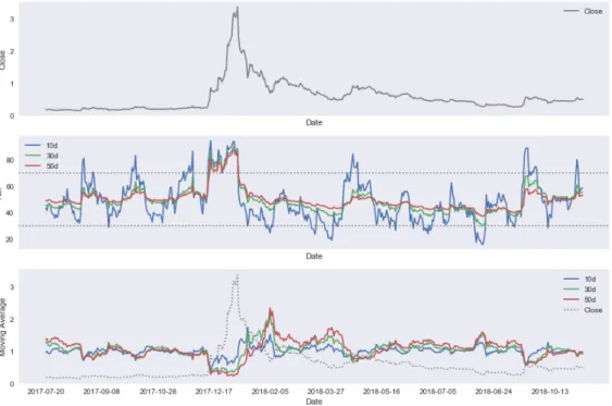
Trend: The moving average is widely used for trend-following systems (Murphy, 1999, chap. 9). The simple moving average which was applied to the price data was computed for a series of time intervals. Time intervals between ten and 200 days3 _{are commonly used. Because the cryptocurrency market is highly volatile,}

the analysis focused on shorter intervals, namely 10, 30 and 50 days. The 200 day interval was computed first but excluded at a later stage to assure more data points can be included.

Momentum:Wilder(1978) describes momentum as one of the most useful concepts but one of the hardest ones to understand. He suggests the Relative Strength Index (RSI) as a momentum oscillator. The RSI measures the magnitude and velocity of directional price movements. To keep the metrics aligned the daily intervals are chosen such that they mimic the moving averages.

Figure3.3visualizes the computed price metrics for the Ripple token as an exam-ple. Traders use the metrics as buy or sell signals. For example, when the shorter interval (e.g. 10 day) moving average falls below the larger interval (e.g. 50 day)

2_{https://mrjbq7.github.io/ta-lib/doc}

index.html

3 https://www.investopedia.com/ask/answers/122414/what-are-most-common-periods-used-creating-moving-average-ma-lines.asp

(26)

moving average, traders would see a sell signal. When the 10 day moving average crosses back above the 50 day moving average, traders would consequently see a buy signal (Murphy,1999, chap. 9 and 10). Wilder (1978) explains RSI thresholds as signals for a stock to be overbought or oversold. When the RSI hits the threshold 70, traders would sell. When it falls below 30 traders would buy. Trendline analysis would take the technical analysis a step further but this exercise was left to a future, more in-depth research into price movements.

Fig. 3.3:Ripple Time Series Decomposition

3.2.3 Factor Metrics

After computing metrics about market movements we are considering further classes in the ITC data. Some of the features such as Token Mining which can take the val-ues ”Mineable” and ”Not-Mineable”, can be insightful but is not yet included in the feature set. As the variable can only take two values we are converting it into a factor variable that can take zero or one as a value (Jameset al.,2013, chap. 3). Another similar variable is the ”Maximal Token Supply”. Some tokens have a max-imal supply whilst others have an infinite supply. Instead of excluding the feature as a whole, a conversion into a factor variable can make it an insightful predictor. If a token has a maximal supply the factor will take value ”1” and ”0” if the supply is infinite.

(27)

3.3 Exploratory Data Analysis 17

The feature engineering leaves us with a dataset of 34 numeric features to be used for further exploration. Due to irregularities in the data further preprocessing steps need to be included to investigate outliers and to bring the data to a workable scale.

3.3 Exploratory Data Analysis

For the exploratory data analysis (EDA) we include the full feature set of 46 vari-ables for 795 tokens. The data includes the numeric features, labels, token names and five day future close prices. The future close price metrics were included in case the data was used for predictions at some stage in the future. In this chapter the data will be preprocessed for model building. This includes identification of missing values, handling of outliers as well as data transformation. The data then undergoes a correlation analysis. The aim is to get an initial understanding for whether the feature space has redundancies. Lastly, the distribution of the token categorization labels will be quantified.

3.3.1 Preprocessing

Classification models are very sensitive to noise in the data. When classifiers are built from low quality data, the model will be less accurate (Teng,1999). To enhance model performance the data will be pre-processed in three steps: identification of missing values, outlier detection and data transformation.

Table3.1shows all missing values in the dataframe, before the ”Maximal Supply” variable was converted into a factor variable. The conversion was already the first step in handling missing values. For the financial metrics calculated the algorithm did not pick up on 165 tokens. This is because some tokens’ time series includes less than 200 days. This means that the token has not been born 200 days before the data was captured. Nevertheless, the metrics can be computed for the 10, 30 and 50-day time intervals. Table3.2 shows that nine tokens are still missing after the 200-day interval was excluded. This means that they have been in the market for less than 50 days. Those tokens will be excluded from the analysis so to keep the feature space broad enough. After the treatment and elimination of missing values, the dataset includes 786 tokens.

To gain a better understanding of the data and its features, pandas4 _and

(28)

3.3 Exploratory Data Analysis 18 Metric Missing SupplyMax 642 5dClosePct 165 5dFutureClose 165 5dCloseFuturePct 165 10dMovAv 165 10dRSI 165 30dMovAv 165 30dRSI 165 50dMovAv 165 50dRSI 165 200dMovAv 165 200dRSI 165

Tab. 3.1:Table of Metrics with Missing Values

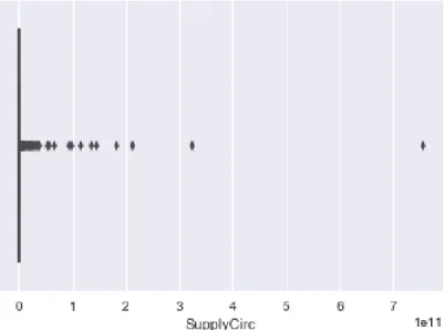
plot5for Python offer useful visualization tools. As a start the data is expressed as a boxplot. The graphs are included in appendixB. Except for the ”Average Rela-tive Volume” and the calculated RSI values, the boxplots basically consist of a flat line. Figure3.4shows the boxplot for the circulating token supply. AsKokoska and Zwillinger(1999, chap. 2) suggest the values outside the box are mild or extreme outliers. In this case most values are very close to zero and all values that are above zero could be considered outliers. Some tokens are trading at an enormous scale compared to others. For example, one Bitcoin would be worth several thousand Dollars whereas one Ripple would range around (and mostly below) one Dollar. Nevertheless, the extreme values must be investigated further. A first check is to see which values are equal or less than zero. In this case, values below zero only make sense for a few values such as the average differences between prices. In fact, there are several features that include values equal to zero. This might be caused by very small numbers that were not processed correctly when the data was extracted. More than 50 tokens have near zero and zero values. Due to their large number, the elimination of those tokens is not considered a valuable option. Next, the extreme values on the upper end need to be evaluated. As the boxplots are so distinct, a threshold of 20% is selected to check which variables cause the data to be imbal-anced. Some of the values are outliers such as the first top ten tokens by market capitalization such as Bitcoin, Ethereum and Ripple. Others such as the Russian

(29)

3.3 Exploratory Data Analysis 19 Metric Missing 5dClosePct 9 5dFutureClose 9 5dCloseFuturePct 9 10dMovAv 9 10dRSI 9 30dMovAv 9 30dRSI 9 50dMovAv 9 50dRSI 9 200dMovAv 163 200dRSI 163

Tab. 3.2:Table of Metrics with Missing Values

Mining Company token stands out due to high prices. Four other outlier tokens are eliminated as their outlier character was not explicable and faulty processing was suspected. Removing these outliers has not caused a significant improvement in the boxplot.

The boxplots also indicate that the data is highly skewed. Skewness can be caused by outliers. Brys et al. (2003) describe skewness as the asymmetry of univariate continuous distributions. This means that the data is not normally distributed. For model building the aim is to find regularities in the distribution of the features. Therefore, the data has to be further processed. AppendixB.2 shows that scaling did not add significant variety to the data, most features still look the same. As an alternative to scaling dataBenoit (2011) suggests a logarithmic transformation of variables using the natural logarithm. The logarithmic transformation is a useful tool to convert highly skewed variables into variables that are closer to a normal distribution (Benoit,2011).

The log-transformation has certain implications on the analysis. For example, log transformation can only be applied to non-zero positive data. Changyong et al. (2014) indicate that one could replace zero values by near zero varibales but this can have significant impact on the outcome. For this analysis, log transformation will only include variables that are non-zero and positive. Table3.3 displays the names of the log-transformed variables.

(30)

Fig. 3.4:Boxplot for Supply Circulation Feature Non-zero, positive features

SupplyCirc 10dMovAv SupplyTotal 30dMovAv AverageVolume 50dMovAv MaximalVolume AvMarketCap LatestVolume MarketCapStDev DifferenceLMVolume MaxMarketCap VolumeStdDev LatestMarketCap

Tab. 3.3: Non-zero, positive features for Log-Transformation

AppendixB.3displays the new boxplot with the transformed data. The logarith-mic transformation was effective and the transformed features suggest a normal distribution of the features. In the next step the data will undergo a correlation analysis.

3.3.2 Correlation Analysis

This subsection will elaborate on a multivariate correlation analysis of the numeric log-transformed dataset in order to detect relationships in the data. Yu and Liu (2004) describe the correlation analysis as a feature selection process. Features are investigated for relevance and redundancy. Furthermore, they describe correla-tions amongst features and a class (Yu and Liu,2004).

(31)

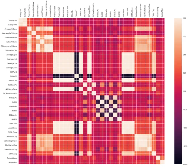
Raschka and Mirjalili (2017, chap. 10) and James et al. (2013, chap. 3) describe important tools for correlation analysis. The aim is to gain a quick overview of whether there are correlations in the data and if so, whether they are positive or negative. A correlation matrix provides insight to detect if there are strongly cor-relating pairs of variables. Figure3.5shows the correlation value between -1 and 1 on a colour scale where the brightest colour represents a stong positive correlation and the dark blue represents a strong negative correlation. Based onTaylor(1990) a strong correlation has a correlation coefficient between 0.68 and 1 and accordingly -0.68 and -1.

Fig. 3.5:Correlation Matrix Visualization for 34 Numeric Features

Strong positive correlations can be observed in certain variable groups. For exam-ple, the token supply circulation correlates with the total token supply. Similarly,

(32)

price and volume metrics are correlating positively. Regarding variables of differ-ent variable groups, the volume and the market capitalization are positively corre-lated. This relationship is not surprising because the more tokens are traded, the higher the price and the number of tokens released or mined.

The average relative volume sticks out from the volume metrics group. It is not correlated with the other volume features. This means that the relative propor-tion of the token volume traded does not increase and decrease with the overall trading volume. Even though the volume increased the proportion of the market capitalization did not change. This is a relevant insight when looking into token performance. Even though the volumes of Bitcoin are much higher as a number, the proportion traded in relation to its market capitalization is similar to many other tokens.

The average high, low, open and close price and the average standard deviation of the close price are positively correlated with the average difference between the maximal and the latest market capitalization. This is an unexpected relationship. We could think of it as the higher the rise the lower the fall. Highly volatile tokens whose average price has been high lost a large portion of their market capitaliza-tion over the past year. When considering the relacapitaliza-tionship in reverse, the tokens with a lower average price and standard deviation did not suffer as big a downfall. The moving averages of 10, 30 and 50 days show a positive correlation. At the same time the RSIs for 10, 30 and 50 days are negatively correlated with the moving av-erages. This originates in the nature of the metrics. Whereas the moving average takes the mean of the prices, the RSI is making an estimate whether a token is over-bought or oversold. A high RSI tells the trader to sell whereas a rising moving average (starting with the shortest interval) is a signal to buy. When analyzing the data, it is evident that the negative correlation of the 10-day Moving Average and the RSI is stronger than the 50-day Moving Average’s.

Another negative correlation is the difference between the average open and close price and the rest of the price metrics. One possible interpretation is that the open and close prices do not rely on the general trend of the data but on other factors such as the activity of traders at a certain time in the day.

High correlations indicate redundancy in the data. Feature selection and variable importance will be addressed in chapter 4. Generally, it is recommended not to

(33)

ex-3.3 Exploratory Data Analysis 23

clude features too early in the analysis because some machine learning algorithms have their own mechanisms to prioritize variables.

3.3.3 Exploration of Classification Labels

Before diving into token classification modelling, this subsection gives a brief overview on the distribution of the different token categories.

Fig. 3.6: Number of Tokens per Primary Label

Figure3.6 shows the number of tokens per category and label. All four primary classification dimensions (economic, tech, legal and industry) are heavily imbal-anced. L ´opez et al. (2012) describe class imbalance as one of the most persistent complications in supervised learning for real-world problems. Lessmann (2004) argues that support vector machines handle class imbalances well for business oriented classification problems andChen and Wasikowski(2008) suggests a new ROC-based feature selection metric. After computing these metrics we learned that other ones outperformed them.

AppendicesB.4andB.5 show the distribution of the secondary, more detailed la-bels. Again, the imbalance is clear.

(34)

Fig. 3.7: Number of Tokens per Primary Economic, Legal and Industry Label After understanding the distribution for each class individually, stacked bar plots help to understand how classes are related. Figure3.7shows the distribution of the legal rights primary label on the primary economic labels. One insight is that pay-ment tokens are not absolute right tokens and with a very high probability, they are no-claim tokens. Investment tokens are in the majority relative right tokens. However, there are some no-claim tokens which is surprising for investment to-kens. Investment tokens are securities by definition where the investor participates in returns and losses. Table3.4shows the six tokens which fall into that category. One reason could be that the companies issuing the tokens navigated through an uncertain legal environment and had to justify a different purpose than they orig-inally intended in order to be able to operate. Another reason could be that the purpose of the token changes over time, or the tokens were mis-classified.

SlugCMC EconomicLabel

c20 EP23M: Investment Token>Derivative Token diamond EP23Z: Investment Token>Other Investment Token karma EP23L: Investment Token>Debt Token

melon EP23P: Investment Token>Fund Token elixir EP23L: Investment Token>Debt Token

bullion EP23Z: Investment Token>Other Investment Token Tab. 3.4:No-claim Investment Tokens

On the right graph in Figure3.7the primary economic label is plotted in relation with the primary industry label. Nearly 100% of the investment and payment

(35)

to-3.3 Exploratory Data Analysis 25

kens are rightly classified into the finance and insurance category. Utility tokens serve multiple different industries.

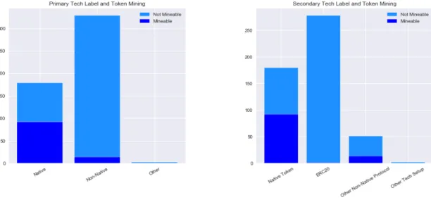
Fig. 3.8: Tech Labels in Relation to Token Mining

Fig. 3.9:Tech Labels in Relation to Maximum Supply

Appendices3.8and3.9investigate the relationship between the primary and sec-ondary technological label with the token mining and the maximum token supply. Mineable tokens are typically protocol tokens but can be both native or non-native protocol tokens. ERC20 tokens together with most non-native tokens are typically not mineable. Native tokens are roughly half mineable and half not-mineable.

(36)

Con-3.3 Exploratory Data Analysis 26

sidering the token supply, the majority of tokens have an infinite supply. Each technological category has a proportion of capped tokens. For native tokens this proportion is 39.1% whilst for non-native tokens only 27.8% have a limited supply.

(37)

Chapter 4 Token Classification Models

Chapter 3 gave a broad understanding of the data. Chapter 4 will provide the clas-sification analysis using machine learning techniques. The section includes variable importance and feature selection, supervised learning methods for classification of the categories as well as unsupervised learning techniques to look beyond that pre-defined classification of tokens.

4.1 Variable Importance and Feature Selection

In this section the feature set will be analysed. For this exercise various different techniques are used and compared. The evaluation of variable importances is done before starting the model building as it is often insightful on its own. Relationships between certain input variables and the desired output classes are found initially. Feature selection has various benefits for prediction models. Models can be signif-icantly faster and more cost-effective by reducing the feature space, for instance by removing redundant variables (Tuvet al., 2009; Guyon and Elisseeff,2003; Chan-drashekar and Sahin,2014). Feature selection can also be seen as an unsupervised learning exercise like in Hierarchical Clustering where the power of features is eval-uated independently from the output variable (Talavera,1999).

Jameset al.(2013, chap. 6) andFriedmanet al.(2001, chap. 10) elaborate on various different feature selection methods. Feature selection techniques can be classified in subset selection, shrinkage and dimension reduction. Table4.1 shows a selec-tion of different methods, most of which were applied to the data. The different techniques vary in performance and interpretability. AppendixC.1visualizes the scores from the chi-sqaured test on the best subset selection algorithm for the pri-mary economic category. The test resulted in high values for the factor variables. The rest of the features scored much lower and it is not obvious which features are

(38)

4.1 Variable Importance and Feature Selection 28

the best to use for the analysis besides the factor variables: token mining and max-imum token supply. I want to elaborate on two more techniques which are known to perform well feature selection.

Subset Selection Shrinkage Methods Dimension Reduction Methods Best Subset Selection

Stepwise Selection

Recursive Feature Elimination

Ridge Regression Lasso

Gradient Boosting

Principle Component Analysis Partial Least Squares

Tab. 4.1:Selected Feature Selection Techniques

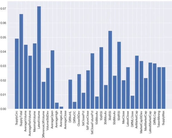
Chen and Guestrin(2016) introduces the XGBoost algorithm1, a tree-based model using boosting and the gradient descent algorithm to improve performance. Figure 4.1shows the feature importances of all the metrics. The XGBoost model accuracy reaches 79.08% when all 34 features are included. When including only 25 features, the performance increases to 81.70% and the model is computationally less expen-sive. The features with the least importance for the model are: the average close, high and low prices, the difference between the average open and close prices and the difference between the average maximal and lowest prices, the 10-day moving average, the 5-day close percentage, the 30-day moving average and the difference between the latest and maximal volume. According to the XGBoost model, not only are those features less relevant, they also add noise so the model performs worse when they are included. The features with the highest importance are the latest volume, the total token supply and the 30-day RSI which is known as the momentum indicator. Consindering the total token supply averages per economic category, payment tokens on average have the highest value ( 6.4bn). With approx-imately 3.9 billion, utility tokens have the second highest supply and investment tokens have the lowest average at about 0.7 billion. Even more significant is the same distribution in the latest volume metric. For payment tokens, the average lat-est volume is at roughly USD 73 billion tokens, for utility tokens USD 8.0 billion and for investment tokens at approximately USD 0.2 billion. Interestingly, the mo-mentum and velocity metric 30-day RSI differs only slightly amongst the economic categories. Per definition, one would suspect that utility and payment tokens have a significantly higher 30-day RSI than investment tokens. In reality, the metric val-ues 47.5 for payment tokens, 45.5 for utility tokens and 46.2 for investment tokens. FiguresC.2to C.4in appendixCshow the XGBoost feature importance plots for the primary labels tech, legal and industry. Table4.2summarizes the maximal

(39)

Fig. 4.1: Shrinkage Method XGBoost

curacies as well as the optimal number of features per prediction model. Whilst the economic and technological categories can be predicted with an accuracy of over 80%, the legal and industry labels are less predictable based on the available data.

Label Maximal Accuracy Number of Variables

Economic 81.70% 25

Tech 86.27% 21

Legal 65.36% 16

Industry 47.71% 19

Tab. 4.2:XGBoost Maximal Accuracies and Optimal Number of Features for Pri-mary Labels

The XGBoost variable importance for the primary tech label in figureC.2 shows that slightly different variables are the most important in this prediction. Although the latest volume is the second most important again, this time the latest market

(40)

capitalization and the 50-day RSI also come into play. Native tokens have signif-icantly higher recent exchange trading volumes (about USD 51 billion) and their average latest market capitalization remains at USD 788 million, whilst non-native tokens were at USD 28 million. This together with the USD 9.5 billions in recent trading volumes for non-native tokens is in line with whatWu et al.(2018) found when analyzing the difference between native tokens (coins) and non-native to-kens. They considered tokens to be an ”explosive immature ecosystem”. The im-portance of the latest market capitalizations and volumes show that the static re-sults during the downward trend in the market distinguishes the tokens from each other. This could mean that native tokens that remain at a higher level are more stable than non-native tokens. One potential reason is considered to be the un-sustainable exponential growth in Initial Coin Offerings (ICOs). ICOs were often carried out without having Minimal Viable Products (MVPs) in place to prove the applications’ value and viability (Wu et al.,2018). When investors lost trust in the market, recently born tokens were more likely to be sold quickly whilst people who invested in the most popular tokens such as Bitcoin and Ethereum held.

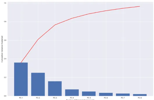
Lastly for this section a principal component analysis (PCA) as indroduced byWold et al.(1987) is used. This technique is a form of dimensionality reduction. The aim is to compute features that are representative of a combination of original features. The advantage is that large feature sets can often be reduced into a two or three dimensional feature space. FigureC.6in the appendix shows a representation of the first two principal components computed for the token data. One dimension (x-axis) is representative of the two factor variables maximal token supply and mineability. The length of the arrow indicates the loading, i.e. how much of the information contained in the feature is included in the principal component. The second component is dominated by the average volume variables, followed by the market capitalization variables and by the supply metrics.

Figure4.2 shows how much of the variance is explained by each principal com-ponent (blue bars) and the cumulatived variance explained (red line). One draw-back of PCA is that beyond two components the interpretability of the data de-creases. Eight principal components explain just over 95% of the variance of the whole dataset of 34 features. In order to maintain better interpretability, we plot the data points into the two-dimensional principal component space and colour the values based on their labels. Figure4.3 shows the two dimensional principal component space for the technological labels. AppendicesC.6to C.8display the same plot but colour coded based on the economic, legal and industry labels. The

(41)

Fig. 4.2:Cumulative Variance Explained for First Five Components

plots show data in three different clusters but none of the labels mimics the clusters exactly. As the clusters are clearly separable based on their x-values one can con-firm that the clusters are based on different combinations of maximal token supply and whether the tokens are mineable or not. There is no such categorization in the ITC, yet. In chapter 5 the possibility of introducing new categories is discussed.

(42)

4.2 Supervised Clustering 32

In the following section on supervised clustering results of different models based on different feature selection methods will be compared. It is found that both the principal components and XGBoost feature variable importance can lead to better results.

4.2 Supervised Clustering

This section describes supervised learning techniques used to predict the economic, technological, legal and industry classes of each token. The aim of supervised learning techniques is to build classifiers based on a set of training data where the outcome class is known (Kotsiantiset al., 2007). The classifiers are then used to predict the class of a test set. The outcome classes in the test set are first hidden and are then used to compare the predicted labels with the actual labels. There are a number of supervised learning classification models whichKotsiantiset al.(2007) evaluated and compared. The results of their work are summarized in tableD.1 in the appendix. The following models are selected: K-Nearest Neighbors (KNN), Neural Networks, Support Vector Machines and tree-based models such as Deci-sion Trees, Bagging, Random Forests and Gradient Boosting. Models like Support Vector Machines and Neural Networks are known for their high prediction accu-racies, especially for large feature spaces. KNN and Decision trees are suitable for smaller feature spaces and are often used for better interpretability. The used fea-ture set is small and therefore good performances for tree-based models and KNN are expected.

Before building each model the data is split into a training and a test set.Fanet al. (2008) developed a well-known package for classification problems suggesting an 80/20 split as in 80% for the training data and 20% for testing. As the data is imbal-anced, the splitting was done in a stratified manner. This means that the proportion of classes was taken into account when splitting it into the test and training set. For KNN and the Neural Network, the target labels were encoded into numeric vari-ables. For the economic label ”0” represents the investment token category, ”1” for payment tokens and ”2” for utility tokens. In the following paragraphs, each model will be briefly described by the example of the economic label using the three dif-ferent feature sets. Each model is built on parameters that were specifically chosen to improve the accuracies. The results are summarized in table4.3.

K-Nearest Neigbors is widely used in classification problems. It is a simpler and therefore a more understandable algorithm but computationally expensive (James

(43)

et al.,2013). The classification algorithm stores all different outcome categories and classifies each data point by a majority vote of its k neighbors (Cover and Hart, 1967). The category that appears most in one group of neighbors gets assigned to all data points in the group. The KNN algorithm can be modified by choosing the dis-tance function that is applied to measure the disdis-tances between the data points and by choosing k, the number of neighbors. The KNNClassifier function allows for Manhatten, Euclidean and Minkowski distance. Amongst the suggested distances Walters-Williams and Li(2010) consider Euclidean as the most popular one and it will be used for the analysis. In order to define the optimal number of neighbors the accuracy for k=1 to k=50 was calculated. Figure4.4shows that the accuracy has two peaks (marked in red) at 26 and 28 neighbors. K=26 neighbors were chosen in order to achieve a test set accuracy of 81.7% when including all features and when using the XGBoost feature selection of 25 variables. For the principal component features the highest accuracy was achieved at 81.0% with k=24 neighbors. Figure 4.5shows the resulting confusion matrix for the XGBoost features. It becomes clear that the algorithm is not picking up on the investment category although it is rep-resented in the test and training set. Again, the reason is the imbalanced data. In the training data 32 data points are labeled investment tokens and 8 in the test set. Nevertheless, the algorithm does not manage to correctly classify the investment tokens.

Fig. 4.4:KNN-Accuracy for XGBoost Feature Selection based on Number of Neigh-bors

(44)

Fig. 4.5:KNN-Confusion Matrix for XGBoost Feature Selection Test Set Tree-based models include Decision Trees, Bagging, Random Forests and the used Gradient Boosting method XGBoost. The Decision Tree builds on the basis of the other three models. The algorithm splits the data into different groups based on the most significant features. This step is repeated until the data is partitioned into a sufficient number of subgroups (Breiman,2017). The splits are estimated through techniques such as the Gini Index which measures the pureness of each group or the Entropy which defines the degree of disorganization in a system (Friedman et al.,2001, chap. 9). The test set accuracy using Entropy to estimate the split out-performs the Gini Index by 0.6%. The accuracy of 79.7% is achieved for all three feature sets using a maximum depth of two for the principal component features and of four for the XGBoost feature selection and all features.

The Bagging algorithm improves the performance of the Decision Tree. The aim is to reduce the variance of the predicted values. This is achieved by combining several tree classifiers modeled on randomly chosen subsets of the training data (Breiman,1996, 1999). The most important modification in the Bagging model is the number of base estimators, in this case the number of trees to be combined. The Bagging algorithm improved all decision tree results. The PCA feature set was improved by 0.7% (n = 6) whilst the XGBoost feature set improved by 1.3% (n = 37) and the original feature set by 2.0% (n = 10) in their accuracies.

Lastly,Breiman(2001) introduced the Random Forests algorithm which is consid-ered to be apanaceafor data science problems. This algorithm is used for predic-tions for both classification and regression problems, for dimension reduction, for treatment of missing values and outlier detection. Instead of building one tree, the