Abstract—The mixed pixel problem is common in remote
sensing. A soft classification can generate land cover class fraction images that illustrate the areal proportions of the various land cover classes within pixels. The spatial distribution of land cover classes within each mixed pixel is, however, not represented. Super-resolution land cover mapping (SRM) is a technique to predict the spatial distribution of land cover classes within the mixed pixel using fraction images as input. Spatial-temporal SRM (STSRM) extends the basic SRM to include a temporal dimension by using a finer-spatial resolution land cover map that pre- or post-dates the image acquisition time as ancillary data. Traditional STSRM methods often use one land cover map as the constraint, but neglect the majority of available land cover maps acquired at different dates and of the same scene in reconstructing a full state trajectory of land cover changes when applying STSRM to time series data. In addition, the STSRM methods define the temporal dependence globally, and neglect the spatial variation of land cover temporal dependence intensity within images. A novel local STSRM (LSTSRM) is proposed in this paper. LSTSRM incorporates more than one available land cover map to constrain the solution, and develops a local temporal dependence model, in which the temporal dependence intensity may vary spatially. The results show that LSTSRM can eliminate speckle-like artifacts and reconstruct the spatial patterns of land cover patches in the resulting maps, and increase the overall accuracy compared with other STSRM methods.
Index Terms—Super-resolution mapping, image series, spatial
dependence, temporal dependence
This work was supported in part by the Strategic Priority Research Program of Chinese Academy of Sciences (Grant No. XDA 2003030201), in part by the Youth Innovation Promotion Association CAS (Grant No. 2017384), in part by the Natural Science Foundation of China (Grant No. 61671425 and 51809250), in part by the Hubei Province Natural Science Fund for Distinguished Young Scholars (Grant No. 2018CFA062), and in part by the British Academy’s Visiting Fellowships Programme under the UK Government's Rutherford Fund to Xiaodong Li to undertake research at the University of Nottingham.
(Corresponding author: Feng Ling, email: [email protected])
X. Li, F. Ling, Y. Zhang, L. Wang, L. Shi, X. Li and Y. Du are with the Key laboratory of Monitoring and Estimate for Environment and Disaster of Hubei province, Institute of Geodesy and Geophysics, Chinese Academy of Sciences, Wuhan 430077, PR China, and with the Sino-Africa Joint Research Centre, Chinese Academy of Sciences, Wuhan 430074, China. X. Li (the first author) is also with School of Geography, University of Nottingham, University Park, Nottingham NG7 2RD, U.K.
G. M. Foody is with School of Geography, University of Nottingham, University Park, Nottingham NG7 2RD, U.K.
Y. Ge is with State Key Laboratory of Resources and Environmental Information System, Institute of Geographic Sciences & Natural Resources Research, Chinese Academy of Sciences, Beijing 100101, China.
I. INTRODUCTION
AND cover and its dynamic play a major role in global change. Understanding the distribution and dynamics of land cover is essential to better understand the Earth’s processes. Remotely sensed images are the main data source in mapping land cover and monitoring land cover changes at different spatial resolutions. However, land parcels managed at a local scale are often smaller than the resolution of satellite data, in which one pixel often represents composite spectral responses from multiple land cover types. Hard classification methods cannot accurately map the mixed pixels, because they assign a mixed pixel to a single land cover class. Soft classification can generate land cover class fraction images that represent the areal proportions of different land cover classes within a pixel. The output of a soft classification is a number of fraction images equal to the number of land cover classes. However, the spatial distribution of land cover classes within the mixed pixel is still unknown. By dividing the pixel into numerous sub-pixels and assuming the sub-pixels are pure, super-resolution mapping (SRM) can assign the class fractions spatially to sub-pixels [1]. SRM can be viewed as the post processing of soft classification that predicts the spatial distribution of land cover classes at the sub-pixel scale. The fraction images output from a soft classification are inputted to an SRM to produce a land cover map with a finer spatial resolution than the original remotely sensed image.
In general, SRM is an ill-posed problem and the result unavoidable contains uncertainty. In order to decrease the uncertainty, various ancillary data such as panchromatic band image [2], vector boundaries [3] and LIDAR [4] have been used in the SRM models to provide more information. However, these SRM methods require that the acquisition dates of these remotely sensed image and ancillary data should be the same or closer, which restricts the use of these data in SRM. Besides the aforementioned ancillary data, land cover maps with finer spatial resolution than the remotely sensed images obtained at different dates are an alternative ancillary data for SRM. The land cover maps can be generated from remotely sensed images obtained from various platforms. Given that land cover map and remotely sensed images can be acquired at different times and considering that a great number of historical land cover maps which cover almost the entire earth may be available, SRM using these land cover maps is very promising.
Spatial-temporal Super-resolution Land
Cover Mapping with a Local Spatial-temporal
Dependence Model
Xiaodong Li, Feng Ling, Giles M. Foody,
Fellow, IEEE
, Yong Ge,
Member, IEEE,Yihang Zhang,
Lihui Wang, Lingfei Shi, Xinyan Li, Yun Du
The spatial-temporal super-resolution mapping (STSRM) first proposed by Ling et al. [5] is an approach that incorporates a finer-spatial resolution land cover map that pre- or post-dates the remotely sensed image acquisition time as ancillary data. Hereafter, we refer the input remotely sensed image has a coarse spatial resolution or coarse resolution, and the input and output land cover maps have fine spatial resolution or fine resolution in STSRM. Note that the terms ‘coarse’ and ‘fine’ do not mean the absolution spatial resolution of the data, but the relative spatial resolution of the image and the land cover map. STSRM is suited to monitor land cover change [6], and has been applied in many fields such as forest mapping [7], change detection [8], and land cover map updating [9].
Various STSRM models have been proposed and can be generally categorized into two groups. The first group of STSRM models are based on the change detection analysis (CDA_STSRM). In CDA_STSRM models, the remotely sensed image pixels are unmixed to coarse resolution land cover fraction images from soft classification, and the fine resolution land cover map is spatially degraded to coarse resolution land cover fraction images. By comparison of these two kinds of fraction images, if the land cover fraction of a class is unchanged in a coarse resolution pixel, the fine resolution pixels that belong to that class in the coarse resolution pixel are assumed to have unchanged class label. Otherwise, the fine resolution pixels that belong to that class in the coarse resolution pixel are assumed to have changed class label, and the label can be determined using various algorithms such as the pixel-swapping algorithm [5], the Hopfield neural network [10], the maximum a posteriori method [9, 11], the learning based model [12], the interpolation based model [13], the swarm intelligence theory [14], the adaptive cellular automata [15], and the artificial neural network [16]. Since error in fraction images is usually unavoidable, a threshold used to distinguish unchanged and changed fractions in each coarse resolution pixel is necessary to be incorporated in CDA_STSRM, and the results depend greatly on the fraction change detection threshold value used. However, the fraction error is usually spatially variable in different pixels and for different classes. The accurately estimation of the threshold in CDA_STSRM is very difficult [10, 11].
The second group of STSRM models are based on spatial-temporal dependence (STD_STSRM). STD_STSRM assumes that fine resolution pixels are spatially dependent with their spatially closest fine resolution pixels, and are temporally dependent with the corresponding fine resolution pixels in images that pre- or post-date the image under analysis. Xu and Huang [17] proposed the spatial-temporal pixel swapping algorithm (STPSA) model that is applied to bi-temporal data, and Wang et al. [18] extended STPSA to multi-temporal data. Li et al. [7] proposed a Markov Random Field based model to map forest cover from Moderate Resolution Imaging Spectroradiometer (MODIS), and Zhang et al. [19] extended this model by using both the 240 m and 480 m spatial resolution MODIS bands. Generally, STD_STSRM predicts all fine pixel labels based on the spatial-temporal dependence model, and removes the need for a change detection threshold.
Considering this advantage, this paper is focused on STD_STSRM.
All STD_STSRM methods predict the fine resolution land cover map based on the a-priori spatial distribution and temporal transition information about land covers. The a-priori information in STD_STSRM includes the a-priori spatial information that is used to predict the land cover spatial patterns at the fine resolution pixel scale and a-priori temporal information that is used to model the temporal transitions between the class labels in the predicted and the input pre- or post-dated land cover maps. The a-priori spatial models have been studied in SRM researches including the spatial dependent model [20-23], the direct mapping model [24], the geostatistical model [25, 26], the multi-point simulation based model [27], the learning based model [28, 29], the adaptive model [30], and the linear spatial distribution model [31, 32]. In these models, [20-24] are suitable for predicting spatial patterns of patches that are larger than the coarse resolution pixel, [25-27] are suitable for predicting spatial patterns of patches that are smaller than the coarse resolution pixel, [31, 32] are suitable for linear patch, and [28-30] are suitable for patches with different spatial patterns, respectively. These a-priori spatial models used in SRM can be directly applied in STD_STSRM. In contrast, the study on the a-priori temporal information in STD_STSRM is very rare. Challenges in STD_STSRM remain, especially if seeking to use a time series of images.
First, in many cases, more than one land cover map of the same scene is available in the area of interest. Since these land cover maps may record the land covers at different dates, incorporating as much fine resolution land cover maps as possible is very useful in accurately mapping land cover trajectories with STSRM. There are three scenarios for the acquisition time of the fine resolution maps and coarse resolution image in STSRM. The first case is that fine resolution maps which pre- and post-date the coarse resolution image are available, the second case is that only a fine resolution map which pre-dates the coarse resolution image is available, and the third case is that only a fine resolution map which post-dates the coarse resolution image is available. For the first case, two available fine resolution maps can be used as the a-priori temporal information to constrain STSRM. By contrast, for the second and third cases, only one fine resolution map is available as the a-priori temporal information. Existing STSRM methods, including both STD_STSRM and CDA_STSRM models, are focused on the second and third cases in which only one fine resolution map is available [5, 9-18, 33-35], but fail to explore the first case. A thorough study on the three cases should be developed in order that the entire land cover change trajectory from remotely sensed image series can be extracted.
Second, the nature of the temporal dependence is often spatially variable. In STD_STSRM models, the temporal dependence is used to link the fine resolution pixels in different date. All existing STD_STSRM models consider the temporal dependence globally, and the intensity of the temporal dependence is, therefore fixed across the entire image. The
global temporal dependence model is used for its simplicity but may not be sufficient to model the spatial and temporal variation that may exist [7]. Generally, the land cover temporal dependence is related to the land cover transition probability. For instance, in the case of forest change, the transition probability from forest to nonforest is usually spatially variable depending on many physical and economic factors such as accessibility and land value [36]. Assuming the transition probability from forest to nonforest is invariant in the area covered by the entire image using the global temporal dependence model is not plausible. It is desirable to change the global temporal dependence to the local scale and to accommodate the spatial variation of its intensity.
Third, land cover fraction errors caused by the soft classification procedure have to be handled in STD_STSRM. In general, the land cover fraction images that are spectrally unmixed from remotely sensed images are inputted in STD_STSRM. As soft classification continues to be an open problem, fraction images errors are often unavoidable in practice. The errors might lead a decrease in the accuracy for existing STSRM methods which constrain the result land cover map in a way that the class fractions within each coarse resolution pixel should be unchanged between the input coarse resolution fraction images and the output fine resolution land cover maps [10]. STD_STSRM should be developed not to strictly preserve the class fractions from the input coarse resolution class fraction images into the result fine resolution land cover map and act to eliminate fraction errors caused by soft classification.
In this paper, a novel Local STD_STSRM (LSTSRM) model is proposed to generate fine resolution land cover maps from a series of coarse resolution class fraction images and a few fine resolution land cover maps. Unlike traditional STSRM models that consider only one fine resolution land cover map, LSTSRM can use both fine resolution maps that pre- and post-date the coarse resolution image to fully explore information in all available datasets and constrain the STSRM problem. In the proposed model, the temporal dependence intensity may vary from pixel to pixel at the fine resolution
scale. In addition, the proposed model is developed not to strictly preserve the class fractions from the input class fraction images into the result land cover map, in order to eliminate fraction errors caused by the soft classification procedure. The remainder of this paper is organized as follows. Section II introduces the LSTSRM method. Section III examines the performance of LSTSRM using synthetic data experiment, real Sentinel-2 images experiment and real MODIS images experiment. Section IV discusses the influencing factors of the proposed method. Section V concludes this paper.
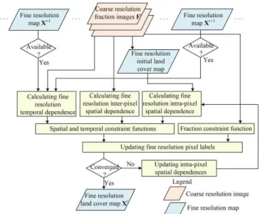
II. METHOD A. The LSTSRM framework
LSTSRM inputs coarse resolution class fraction images Ft at the observation time t (t=1,2,…,T), as well as the fine resolution land cover maps Xt-1 and/or Xt+1 that covers the same
geographical region but obtained at times that pre- and/or post-date Ft, as input, and outputs the fine resolution land cover map Xt, at time of t. The coarse resolution fraction images Ft can be produced from remotely sensed image using various soft classification procedures. The fine resolution maps Xt-1and
Xt+1 can often be produced from fine resolution remotely
sensed image by, for example, classification or manual digitization. Although a series of fine resolution land cover maps may be available and can be incorporated in LSTSRM, only those which are acquired temporally closest to and pre- or post-date Yt are selected as X t-1 and/or Xt+1. This is because the
land cover datasets are temporally more dependent if they are obtained at temporally closer time [6, 18]. Ft contains I × J × C pixels (I × J is the number of coarse resolution pixels and C is the number of land cover classes). Xt, Xt-1 and Xt+1 each
contains I × s × J × s pixels, where s is the scale factor and each coarse resolution pixel contains s × s fine resolution pixels. Each pixel in Xt, Xt-1and Xt+1 has a land cover class label in C.
In LSTSRM, the three scenarios, that is, both Xt-1and Xt+1are
available (case 1), only Xt-1is available (case 2), and only Xt+1 is available (case 3), are considered (Fig. 1).
Based on Bayesian theory, the optimal Xt can be expressed as:
Fig. 1. The spatial and temporal neighborhoods for a fine resolution pixel. Case 1: Both Xt-1and Xt+1 are available. Case 2: Xt+1is available. Case 3: Xt+1 is available. The fine resolution pixel highlighted in black in Xt is the target pixel. The fine resolution pixels highlighted in blue and the coarse resolution pixels highlighted in
1 +1
arg max , , t t t t t P X X F X X (1) where P(Xt|Ft,Xt-1,Xt+1) is the posterior probability of Xt, givenFt, Xt-1 and/or Xt+1. The Markov random field can model
contextual information by characterizing the local statistical dependence among pixels in terms of conditional prior distribution [37]. The Markov random field can simplify the global model in (1) to a model of the local image properties, and largely reduces the model complexity to make the maximum a posteriori (MAP) model solvable. The optimal Xt, given Ft, Xt-1and/or Xt+1, can be formulated by applying the
MAP rule, i.e., by solving the maximization problem:
1 +1 1 +1 arg max , , 1arg max exp , ,
t t t t t t t t t P U Z X X F X X X F X X (2)
where U(Xt|Ft,Xt-1,Xt+1) is the posterior energy function of Xt and Z is a normalizing constant. Based on the Markov random field approach, the searching of the optimal Xt is equivalent to minimization the posterior energy function, which can be specified to model the spatial and temporal dependencies of pixel on its spatial and temporal neighborhoods. U(Xt|Ft,Xt-1,Xt+1) is calculated as:
-1 +1
-1 +1 ( ) ( ) ( ) , , , t t t t t t t t t T t S F U U U X F X X X X X X U F X (3) where US(Xt) and UT(Xt|Xt-1,Xt+1) are the spatial and temporal constraint functions, and UF(Ft|Xt) is class fraction constraint function that represents the inconsistency between Ft and Xt.B. The Spatial and Temporal Constraint Functions
The LSTSRM spatial and temporal constraint functions are used to incorporate land cover a-priori spatial and temporal dependence model according to the spatial-temporal neighborhood system (Fig. 1). Each fine resolution pixel in Xt highlighted in black is spatially dependent on its spatial neighborhood fine resolution pixels marked in blue and spatial neighborhood coarse resolution pixels highlighted in yellow in Xt, and is temporally dependent on its temporal neighborhood fine resolution pixels highlighted in red in Xt-1and Xt+1.
1) Spatial Constraint Function
The LSTSRM spatial constraint function is based on the spatial dependence principle which is the tendency of spatially proximate observations of a given property to be more similar than distant observations. It assumes that a fine resolution pixel and its neighboring fine resolution pixels have high probabilities to be labeled with the same class. At present, there are two methods to describe the spatial dependence of pixels, namely intra-pixel spatial dependence and inter-pixel spatial dependence, which are used to represent the spatial dependence within and between image pixels, respectively [20, 38-40]. Assume pt
ijk is the kth (k=1,…,s2) fine resolution pixel in coarse
resolution pixel (i,j) (i=1,…,I, j=1,…,J) in Xt. DS intra(c(p
t ijk)=c) is
the intra-pixel spatial dependence of fine resolution pixel pt ijk
when it has a label of c (c=1,…,C), and DS inter(c(p t
ijk)=c) is the
inter-pixel spatial dependence of fine resolution pixel pt ijk when
it has a label of c. The spatial energy function US(Xt) can be written as:
2 1 2 1 1 1 1 ( ) 1 I J s C S t S tS intra ijk inter i k
i j k c t j U D c p c D c p c
X (4) where α1andα2 define the weight of the intra- and inter-pixelspatial dependence values. In Eq. (4), -1 is multiplied because the LSTSRM seeks the minimum value as the optimal solution. The determination of intra-pixel spatial dependence and inter-pixel spatial dependence is explained as follows. 1.1)Intra-pixel Spatial Dependence:
The intra-pixel spatial dependence is computed at the sub-pixel/sub-pixel (fine resolution pixel/fine resolution pixel) scale, meaning the spatial dependence of a sub-pixel (highlighted in black in Fig. 1) is determined by its neighborhood same-class sub-pixels (highlighted in blue in Fig. 1). The intra-pixel spatial dependence DS
intra(c(p t
ijk)=c) is
determined by the pixel labels of its neighboring eight fine resolution pixels in the neighborhood system:
( ) ( ), 8 t ijk S t t intra ijk l l p D c p c c p c
N (5) where N(ptijk) is the fine resolution spatial neighborhood, and p t l
is a neighborhood fine resolution pixel in N(pt ijk). c(p
t
ijk) and
c(pt
l) are the land cover class labels for fine resolution pixels p t ijk and pt l. δ(c(p t l),c) equals 1 if c(p t
l) and c are the same and 0
otherwise.
1.2) Inter-pixel Spatial Dependence:
The inter-pixel spatial dependence is calculated at the sub-pixel/pixel scale, meaning that the inter-pixel spatial TABLEI
LIST OF THE IMPORTANT VARIABLES
Variable name Definition
Ft The input coarse resolution class fraction images at
time of t;
Xt The predicted fine resolution land cover map at time
of t;
Xt-1 The input fine resolution land cover map at time of
t-1; Xt-1 pre-dates Xt;
Xt+1 The input fine resolution land cover map at time of
t+1; Xt+1 post-dates Xt; pt
ijk
The kth fine resolution pixel in coarse resolution pixel (i,j) in Xt;
DS intra(c(p
t ijk)=c)
The intra-pixel spatial dependence of fine resolution pixel pt
ijk when it has a label of c (c=1,…,C, and C is
the total number of classes in the image).
DS inter(c(p
t ijk)=c)
The inter-pixel spatial dependence of fine resolution pixel pt
ijk when it has a label of c (c=1,…,C) ;
DT G(c(p
t ijk)=c)
The global temporal dependence intensity of fine resolution pixel pt
ijk if p t
ijk belongs to the cth class;
DT L(c(p
t ijk)=c)
The local adjust factor of fine resolution pixel pt ijk if p
t ijk
belongs to the cth class;
MTSRM Mono-temporal super-resolution mapping; STSRM Spatial-temporal super-resolution mapping; LSTSRM Local temporal dependence model based STSRM; GSTSRM Global temporal dependence model based STSRM.
dependence of a sub-pixel (highlighted in black in Fig. 1) is determined by the same-class fine resolution pixels in the neighboring coarse resolution pixel (highlighted in yellow in Fig. 1) [39]. Spatial interpolation algorithms such as inverse distance weighted function or Kriging can be used to represent the relationship between sub-pixel and pixels [39, 41]. By spatially interpolating the neighborhood coarse pixel class fractions of each class to the sub-pixel scale, the inter-pixel spatial dependence DS
inter(c(p t
ijk)=c) is defined as:
( )S t t
inter ijk c ijk
D c p c f p (6) where fc(pt ijk) is the spatially interpolated fractions of the cth class
at sub-pixel pt
ijk. The value of fc(pt ijk) is related to the cth class
fractions in the neighborhood coarse pixels, the distance between pt
ijk and the neighborhood coarse pixels, and the
spatially interpolation method being used [42]. 2) The Spatial and Temporal Constraint Functions
The LSTSRM fine pixel temporal dependence intensity is defined according to DT G(c(p t ijk)=c) and D T L (c(p t ijk)=c),where DT G(c(p t
ijk)=c) is the global temporal dependence intensity of fine
resolution pixel pt ijk if p
t
ijk belongs to the cth class, and D T L(c(p
t ijk)=c)
is the local adjust factor of fine resolution pixel pt ijk if p t ijk belongs to the cth class:
2 1 -1 +1 1 1 1 1 , ( ) T I J s C T t T t G ijk i t t L jk i j k t c U D c p c D c p c
X X X . (7) where β is the temporal constraint function weight parameter. The global temporal dependence intensity DTG (c(p
t
ijk)=c) is
assigned to 1 if the kth fine resolution pixel in coarse resolution
pixel (i,j) belongs to the cth class in Xt-1or Xt+1, and is assigned
to 0 otherwise. Therefore, the fine resolution pixels in Xt and
Xt-1(or Xt+1) are temporally dependent if they have the same
class label, and are temporally independent if they have different class labels. The local adjust factor DT
L (c(p
t ijk)=c)
depends not only on the fine resolution class labels in Xt-1
and/or Xt+1, but also on the coarse resolution class fractions at
times of t-1, t and t+1. The calculation of the local adjust factor DT
L(c(p t
ijk)=c) according to different input data are explained as
follows.
2.1) Both Xt-1and Xt+1are Available:
Before the calculation of the local adjust factor DT L(c(p
t ijk)=c),
the fine resolution pixels in coarse pixel (i,j) in Xt are grouped into different sets according to the spatial distribution of fine resolutions of the cth class in Xt-1and Xt+1, assuming different
set of fine pixels may have different temporal dependence and different local adjust factors. An example on grouping different fine resolution pixel sets is shown in Fig. 2. Fig. 2 (a) and (c) shows fine pixels that belong or not belong to cth class in the
coarse pixel (i,j) in Xt-1 and Xt+1. By comparing Fig. 2 (a) and
(c), four sets of fine resolution pixels in coarse resolution pixel (i,j), which are pt-1&t+1
ij,c , p t-1 ij,c, p t+1 ij,c and p non
ij,c, are defined in Fig. 2(b).
The detailed definitions are given in Fig. 2. Let f(pt
ij,c) be the fractions of the cth class in coarse resolution
pixel (i,j) in Ft that is unmixed using soft classification. Let
f(pt-ij,c1&t+1), f(p t-1
ij,c) and f(p t+1
ij,c) be the fractions of the cth class in
coarse resolution pixel (i,j), which are calculated by dividing the number of pixels in pt-1&t+1
ij,c , p
t-1
ij,c and p t+1
ij,c in coarse resolution
pixel (i,j) by s2 (s is the scale factor). The local adjust factor is
quantified by comparing f(pt ij,c) with f(p t-1&t+1 ij,c ), f(p t-1 ij,c) and f(p t+1 ij,c).
In LSTSRM, a simple rule is used in which a fine pixel that belongs to the cth class is more probably to be in the set pt-1&t+1
ij,c
than in the sets pt-1
ij,c and p
t+1
ij,c. In addition, a fine resolution pixel is
not likely to belong to the cth class if this pixel does not belong
to the cth class in Xt-1and Xt+1, and the local adjust factor for
fine resolution pixels in pnon
ij,c is set to 0. Based on this rule, the
local adjust factor according to the following cases is calculated. If f(pt ij,c)≥ f(p t-1&t+1 ij,c )+f(p t-1 ij,c)+f(p t+1
ij,c ), then the fine resolution
pixels in the sets pt-1&t+1
ij,c , p
t-1
ij,c, p t+1
ij,c are all temporally dependent.
The fine resolution pixels in pt-1&t+1
ij,c , p
t-1
ij,c and p t+1
ij,c should all
belong to the cth class in Xt, and the corresponding local adjust Fig. 2. An illustration of building the local adjust factor for the temporal dependence according to the fine resolution pixels labels of the cth class in pixel (i,j). (a) One coarse resolution pixel in Xt+1. (b) One coarse resolution pixel in Xt. (c) One coarse resolution pixel in Xt+1. Each coarse resolution pixel contains 10×10 fine resolution pixels.
factor equals to 1, which is the maximal local adjust factor value.
If f(pt
ij,c) is lower than f(p t-1&t+1
ij,c )+f(p
t-1
ij,c)+f(p t+1
ij,c) but higher than
f(pt-1&t+1
ij,c ), the fine resolution pixels in p t-1&t+1
ij,c should belong to the
cth class and the corresponding local adjust factor remains to be
1, whereas the fine resolution pixels in pt-1
ij,c and p t+1
ij,c are not
definitely to belong to the cth class and the corresponding local
adjust factor is lower than 1. More specifically, the probability of fine resolution pixels in pt-1
ij,c and p t+1
ij,c belonging to the cth class
is proportional to the difference between f(pt
ij,c) and f(p t-1&t+1
ij,c ) in
Eqs (8-9). In addition, the probability of fine resolution pixels in pt-1
ij,c and p t+1
ij,c belonging to the cth class decreases with the time
interval between Xt and Xt-1 or between Xt and Xt+1, assuming
the temporal dependence decreases with the time interval between images. Let Δt(Xt-1, Xt) and Δt(Xt, Xt+1) be the time
interval from the acquisition time from Xt-1to Xt and from the acquisition time from Xt to Xt+1, respectively. The local adjust
factor for the sets pt-1
ij,c and p t+1
ij,c are calculated as
1& 1
-1 , , -1 +1 1 1 , , ( , ) 1 ( , ) ( , ) t t t t t ij c ij c T t L ijk t t t t t t ij c ij c f p f p t D c p c t t f p f p X X X X X X (8) if pt ijk belongs to p t-1 ij,cand as
1& 1
+1 , , -1 +1 1 1 , , ( , ) 1 ( , ) ( , ) t t t t t ij c ij c T t L ijk t t t t t t ij c ij c f p f p t D c p c t t f p f p X X X X X X (9) if pt ijk belongs to p t+1 ij,c.If f(pt ij,c) is lower than f(p t-1&t+1
ij,c ), the fine resolution pixels in
the set pt-1&t+1
ij,c are temporally dependent with the corresponding
fine pixels in Xt-1 and Xt+1, and the probability that fine
resolution pixels in pt-1&t+1
ij,c belongs to the cth class is proportional
to the value of f(pt ij,c):
,
1& 1 , t ij c T t L ijk t t ij c f p D c p c f p . (10) In contrast, the fine resolution pixels in the sets pt-1ij,c and p
t+1
ij,c are
temporally independent, and the corresponding local adjust factorequals to 0.
2.2) Only Xt-1is Available:
Only the number of fine resolution pixels of pt-1
ij,c in Xt-1 is
considered. If f(pt ij,c)> f(p
t-1
ij,c), the local adjust factorequals to 1 if
pt
ijk belongs to p t-1
ij,c and 0 otherwise. If f(p t ij,c)≤ f(p
t-1
ij,c), the local
adjust factoris calculated as:
, 1 , t ij c T t L ijk t ij c f p D c p c f p (11) if pt ijk belongs to p t-1ij,cand 0 otherwise.
2.3) Only Xt+1is Available:
Only the number of fine resolution pixels of pt+1
ij,c in Xt+1is
considered. If f(pt ij,c)> f(p
t+1
ij,c), the local adjust factorequals to 1 if
pt
ijk belongs to p t+1
ij,c and 0 otherwise. If f(p t ij,c)≤ f(p
t+1
ij,c), the local
adjust factoris calculated as:
, 1 , t ij c T t L ijk t ij c f p D c p c f p (12) if pt ijk belongs to p t+1ij,c and 0 otherwise.
Although only Xt-1or Xt+1is considered in cases (2) and (3),
the LSTSRM temporal dependence model is different from those in [7, 11, 17, 18, 43], because the local information is considered in LSTSRM but not in the previous studies. C. Fraction Constraint Function
The land cover fraction constraint function represents the difference between the class fractions in the input fraction images Ft and the final fine resolution map Xt:
, , F 2 1 1 ( ) t t I t t t t ij i ij J j U
F X F X f f (13)where ftij,Ft is a C × 1 vector of different class fraction values in
the coarse resolution pixel (i,j) in Ft. ft
ij,Xt is a C × 1 vector of
different class fraction values in the coarse resolution pixel (i,j) in Xt calculated by dividing the number of fine resolution pixels of different classes in coarse resolution pixel (i,j) by s2 in Xt.
2
indicates the L2 norm.
D. Fine Resolution Map Initialization and Updating
The flowchart of LSTSRM is shown in Fig. 3. An initial fine resolution land cover map is used as input to LSTSRM at the outset. The initial map is produced according to the land cover class fraction images. The fine resolution pixels are allocated class labels randomly in a manner that maintains the class proportional information conveyed by fraction values [44]. The class labels in the initial fine resolution land cover map are then updated iteratively. The iterative conditional mode, a simple gradient-based optimization algorithm, was applied for updating the fine resolution pixel class labels.
III. EXPERIMENT AND RESULTS
The proposed LSTSRM model was assessed in three experiments. The first used the National Land Cover Database (NLCD) of U.S.A. [45], the second used Sentinel-2 and Google Earth images, and the third used MODIS and Landsat images. In each experiment, in order to explore the influence of input fine resolution map on the proposed method, LSTSRM using
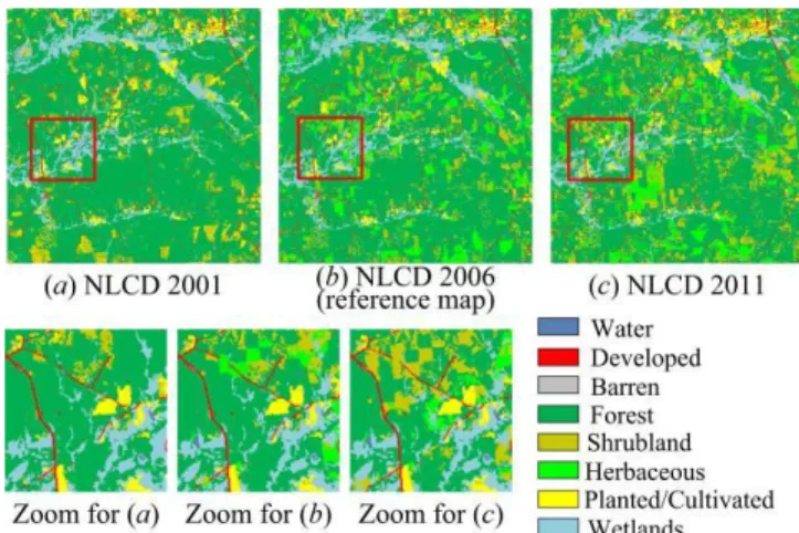
Fig. 4. The reference maps and change maps of the NLCD data.
two fine resolution maps (i.e., LSTSRMt-1&t+1, the superscripts
‘t-1’ and ‘t+1’ indicate the fine resolution land cover maps that
pre- and post-dates the prediction map) was compared with LSTSRM using only one fine resolution map (i.e., LSTSRMt-1
and LSTSRMt+1). In addition, the proposed method using two
fine resolution maps but using global land cover temporal dependence model (i.e., GSTSRMt-1&t+1) was also compared. In
GSTSRMt-1&t+1, the local adjust factor, which may vary for
different fine pixels and for different classes in LSTSRM, is set to 1 for all fine resolution pixels and for different classes in the entire image in Eq. (7).
Several popular SRM algorithms were used for comparison including the pixel swapping algorithm based SRM (PSA) [20], the Kriging interpolation based SRM (KI) [41, 46, 47], the Hopfield neural network based SRM (HNN) [25], the spatial-temporal pixel swapping algorithm (STPSA) [17], the subpixel land cover change mapping algorithm (SLCCM) [5], and the SRM based on spatial–temporal dependence from a former map (SRM_STD) [34]. Among different methods, PSA, KI and HNN are applied to mono-temporal coarse resolution land cover fraction images, which are referred as mono-temporal SRM (MTSRM) methods, and STPSA, SLCCM and SRM_STD are applied to coarse resolution land cover fraction images and a fine resolution land cover map, which are referred as spatial-temporal SRM (STSRM) methods. The LSTSRM weight parameters in all experiments were set through trial and error.
A. Simulated NLCD Experiment 1) Data Preparation
The 30 m resolution NLCD maps were adopted in this experiment. NLCD is a land cover classification scheme of Albers Equal Area projection, which has been applied consistently at a spatial resolution of 30 m across the conterminous USA primarily on the basis of Landsat satellite data. The study area is located in Charlotte (33º7'00"N and 81º3'00"W), U.S.A. The NLCD maps acquired in 2001, 2006 and 2011, each contains 800 × 800 pixels in size, were used as the fine resolution land cover maps (Fig. 4(a-c)). The original NLCD maps contain sixteen classes according to the NLCD classification system modified from the Anderson Land Cover Classification System [45]. The original sixteen classes were reclassified to eight classes, namely water, developed, barren, forest, shrubland, herbaceous, planted/cultivated, and wetlands in this experiment.
This experiment was intended to predict the NLCD 2006 map, using coarse resolution fractions images in 2006 and fine resolution NLCD maps in 2001 and 2011.The coarse resolution fraction images in 2006 were simulated based on NLCD 2006. The coarse resolution fraction image of each class in the year 2006 was produced by dividing the number of fine resolution pixels that belong to that class in each coarse resolution pixel in NLCD 2006 according to the scale factor s, which was set s=10. This approach can produce error-free fraction images compared with those produced by soft classification [20, 24].
The input of different methods was set. For all methods, the coarse resolution class fraction images in the year 2006 were inputted. For SRM methods, STPSA, SLCCM and SRM_STD
and LSTSRM using fraction images in the year 2006 and NLCD 2001 map (i.e., STPSAt-1, SLCCMt-1, SRM_STDt-1, and
LSTSRMt-1) and using fraction images in the year 2006 and
NLCD 2011 map (i.e., STPSAt+1, SLCCMt+1, SRM_STDt+1 and
LSTSRMt+1) were tested. LSTSRMt-1&t+1 and GSTSRMt-1&t+1
using both the 2001 and 2011 NLCD maps were compared. The accuracies of different methods were assessed using the NLCD 2006 (Fig. 4 (b)).
2) Results
The resulting maps in the zoomed area from different methods are shown in Fig. 5. The KI map contained unsmoothed boundaries because it discarded the intra-pixel spatial dependence which can help to generate locally smoothed boundaries in the result (Fig. 5(b)). The PSA map failed to reconstruct the holistic land cover spatial patterns because it discarded the land cover inter-pixel spatial dependence (Fig. 5(c)). The PSA map contained many land cover patches with small size represented as speckle-like artifacts. In contrast, the HNN map eliminated the speckle-like artifacts (Fig. 5(d)). This difference lays in the fact that KI and PSA must preserve class fractions in the resulting map, and the land covers with small area proportion or fraction in a coarse resolution pixel would be aggregated to small land cover patches represented as speckle-like artifacts. In contrast, HNN does not strictly preserve the class fractions from the input class fraction images into the result land cover map, and would eliminate the speckle-like artifacts due to spatial smoothing effect [20, 25]. However, since KI, PSA and HNN only considers the land cover spatial information but neglect land cover temporal information in the land cover map that pre- and/or post-dates the prediction date, the spatial details were not represented in the result maps.
The STSRM methods, including STPSA, SLCCM, SRM_STD and LSTSRM, preserved the spatial details of land cover classes in Fig. 5 (Fig. 5(e-n)). All these maps were very similar to the reference NLCD 2006 map. The linear developed class was connected in these maps, and the shapes of objects such as herbaceous, planted/cultivated, and water were reconstructed.
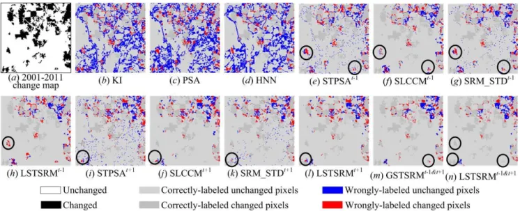
Fig. 6 shows the error maps from different methods. The MTSRM algorithms of KI, PSA and HNN generated more error pixels (highlighted in red and blue in Fig. 6(b-d)) compared with those STSRM methods in Fig. 6(e-n). In addition, the MTSRM generated more wrongly-labeled unchanged pixels highlighted in blue than wrongly-labeled changed pixels highlighted in red in Fig. 6(b-d)), whereas STSRM eliminated most wrongly-labeled unchanged pixels highlighted in blue in Fig. 6(e-n), showing that incorporating temporal dependence in SRM can reduce the commission error especially for unchanged pixels. Among all the result maps, the LSTSRMt-1&t+1 contained the least wrongly-labeled fine pixels
in Fig. 6(n), and the wrongly-labeled fine pixels highlighted in the circles in other STSRM maps (Fig. 6(e-l)) were eliminated in the LSTSRMt-1&t+1 map. This result not only shows that the
proposed LSTSRMt-1&t+1 increased the accuracy than the
existing STSRM algorithms of STPSA, SLCCM and SRM_STD, but also shows that the proposed STSRM using two fine maps is superior to that using only one fine map, and the proposed STSRM using local temporal dependence model is superior to that using global temporal dependence model.
The overall accuracies of different methods are shown in Table II. The overall accuracies of MTSRM methods were lower than 81%, whereas those of STSRM methods were Fig. 5. The result maps in the zoomed area from different methods. The superscripts ‘t-1’ and ‘t+1’ indicate NLCD 2001 and 2011 maps used in the methods.
Fig. 6. The error maps in the zoomed area from different methods. The superscripts ‘t-1’ and ‘t+1’ indicate NLCD 2001 and 2011 maps used in the methods. TABLEII
THE OVERALL ACCURACIES (%)OF DIFFERENT METHODS IN THE NLCD EXPERIMENT.
KI PSA HNN STPSAt-1 STPSAt+1 SLCCMt-1 SLCCMt+1 SRM_STDt-1 SRM_STDt+1 LSTSRMt-1 LSTSRMt+1 GSTSRMt-1&t+1 LSTSRMt-1&t+1
higher than 89%. The accuracies of STPSAt-1, SLCCMt-1 and
SRM_STDt-1 were similar, and the accuracies of STPSAt+1,
SLCCMt+1 and SRM_STDt+1 were similar, showing that the
input fine resolution map plays a key role for STPSA, SLCCM and SRM_STD. In addition, the overall accuracy for LSTSRMt-1 was higher than those of STPSAt-1, SLCCMt-1 and
SRM_STDt-1, and the overall accuracy for LSTSRMt+1 was
higher than those of STPSAt+1, SLCCMt+1 and SRM_STDt+1. It
shows that LSTSRM improves the accuracy compared with STPSA, SLCCM and SRM_STD when only one fine map is used in STSRM. LSTSRMt-1&t+1 generated the highest overall
accuracy among all methods, showing the advantage of the proposed method.
B. Sentinel-2 Experiment 1) Data Preparation
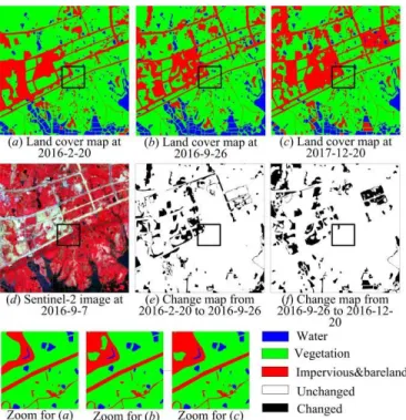
The LSTSRM was tested using real Sentinel-2 remotely sensed images in this experiment. Sentinel-2 was launched by the European Space Agency in 2015, and can provide global acquisitions of fine resolution multi-spectral images with a fine revisit frequency. The Sentinel-2 image is useful in land cover mapping due to its appealing properties (10 days at the equator with one satellite, and 5 days with 2 satellites which result in 2-3 days at mid-latitudes) and the free access. In this experiment, Sentinel-2 image was utilized to map land covers in an urban area located in Wuhan (30°27′30″N and 114°32′30″E), Hubei province, China. The Sentinel-2 image acquired on September 7 2016 with four 10 m spatial resolution Sentinel-2 bands (blue, green, red and infrared bands) was used to generate land cover map in the study area (Fig. 7(d)). A Google Earth image acquired on September 26 2016 was digitized to a 2 m spatial resolution land cover map for accuracy assessment (Fig. 7(b)). Two fine resolution Google Earth
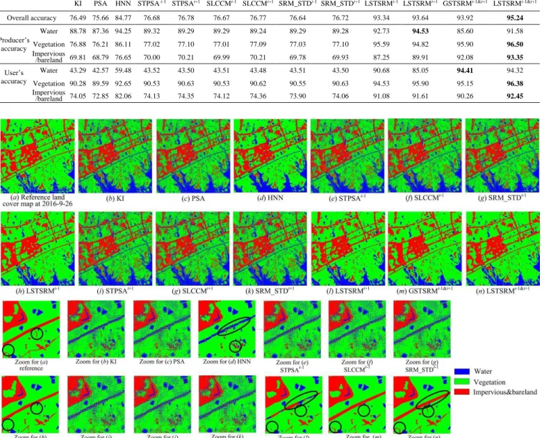
images that acquired on February 20 2016 and December 20 2017, respectively, were digitized to 2 m spatial resolution land cover maps as the STSRM input (Fig. 7(a),(c)). The study area covers 400 × 400 Sentinel-2 pixels, which correspond to 2000 × 2000 fine resolution pixels in the input and reference maps, with a scale factor s = 5. There are three land cover types, which are water, vegetation and impervious/bareland, contained in the input and reference land cover maps.
The proposed LSTSRM using both fine maps and using local temporal dependence model, i.e., LSTSRMt-1&t+1, was
compared with the same methods used in the first experiments, including MTSRM of KI, PSA and HNN, as well as the STSRM methods of STPSAt-1, STPSAt+1, SLCCMt-1,
SLCCMt+1, SRM_STDt-1, SRM_STDt+1, LSTSRMt-1,
LSTSRMt+1 and GSTSRMt-1&t+1 (the superscripts ‘t-1’ and ‘t+1’
indicate the Google Earth 2016 and 2017 maps, respectively). For the MTSRM and STSRM methods, the multiple endmember spectral mixture analysis was applied to generate land cover class fraction images [48].
2) Results
Fig. 8 shows the result maps and zoomed images from different methods. Different to the NLCD experiment which used error-free coarse spatial resolution land cover fraction images, this experiment used fraction images that were unmixed from the Sentinel-2 image which inevitably contained errors in Fig. 8. The zoomed image for KI (b) and PSA (c) contained many speckle-like artifacts which were resulted from soft classification error. For instance, if a coarse pixel does not contain pixels of water class and the unmixed water fraction is 12% in this coarse pixel, then a total number of 52×12% =3 (5 is
the scale factor) fine pixels are labeled as water class within this coarse pixel, which may be represented as speckle-like artifacts since these methods must preserve class fractions in the resulting map. KI and PSA preserved class fractions in the resulting map, resulting in speckle-like artifacts due to soft classification errors in the class fraction images. HNN eliminated the speckle-like artifacts because it had the spatial smoothing effect and did not strictly preserve the class fractions from the input class fraction images into the result land cover map. However, the impervious&bareland patch highlighted by the ellipse in the zoomed area in Fig. 8(d) was wrongly labeled as water, and the detailed spatial pattern of the linear impervious&bareland patch highlighted by the circle was not reconstructed.
Among the STSRM results in Fig. 8, the STPSA, SLCCM and SRM_STD (Fig. 8(e-g),(i-k)) contained a large number of speckle-like artifacts due to soft classification error, whereas LSTSRM (Fig. 8(h),(l),(n)) and GSTSRM (Fig. 8(m)) eliminated these errors due to spatial smoothing effect. Similar to HNN, LSTSRM and GSTSRM eliminated the speckle-like artifacts because they have the spatial smoothing effect and do not to strictly preserve the class fractions from the input class fraction images in the result land cover map. The LSTSRM and GSTSRM maps in Fig. 8 (h) and (l-n) were much similar to the reference map than the HNN map in Fig. 8(d). This is because LSTSRM and GSTSRM incorporated land cover temporal information from the input land cover map whereas HNN did not. As soft classification error is usually unavoidable in real applications, LSTSRM and GSTSRM would be more suitable Fig.7. The reference fine resolution maps, Sentinel-2 images and change maps.
for land cover mapping of image series compared with STPSA, SLCCM and SRM_STD in practice.
In the zoomed images, LSTSRMt-1, LSTSRMt+1 and
GSTSRMt-1&t+1 failed to reconstruct the linear
impervious&bareland patch highlighted by the circles in Fig. 8(h),(l) and (m). LSTSRMt+1 erroneously labeled a part of
impervious&bareland as water highlighted by the ellipse in the zoomed image for Fig. 8(l). LSTSRMt-1 and GSTSRMt-1&t+1
erroneously labeled a part of impervious&bareland as vegetation highlighted by the circle in the zoomed image for Fig. 8 (h), (m). LSTSRMt-1&t+1 correctly labeled the
impervious&bareland patch highlighted by the ellipse and reconstructed most parts of the linear impervious&bareland patch highlighted by the circles in the zoomed image for (n), and was similar to the reference image.
The overall accuracy, producer’s and user’s accuracies of different methods are presented in table III. The overall accuracies for KI, PSA, STPSA, SLCCM and SRM_STD, which strictly preserve the class fractions from the input class fraction images in the result land cover map, were lower than 80%, showing that the soft classification error strongly affects these MTSRM and STSRM methods. HNN had an overall accuracy of about 85%, and LSTSRM and GSTSRM increased the overall accuracy to higher than 93%. Among LSTSRM and GSTSRM, for the water class, LSTSRMt+1 has the highest
producer’s accuracy but the lowest user’s accuracy served as a high commission error of water. This is shown in the zoomed image of (l) in which some impervious&bareland pixels were wrongly labeled as water highlighted by the ellipse in LSTSRMt+1. In addition, among LSTSRM and GSTSRM and
TABLEIII
THE ACCURACIES (%)OF DIFFERENT METHODS IN THE SENTINEL-2IMAGE EXPERIMENT.
KI PSA HNN STPSA t-1 STPSAt+1 SLCCMt-1 SLCCMt+1 SRM_STDt-1 SRM_STDt+1 LSTSRMt-1 LSTSRMt+1 GSTSRMt-1&t+1 LSTSRMt-1&t+1
Overall accuracy 76.49 75.66 84.77 76.68 76.78 76.67 76.77 76.64 76.72 93.34 93.64 93.92 95.24 Producer’s accuracy Water 88.78 87.36 94.25 89.32 89.29 89.29 89.24 89.29 89.28 92.73 94.53 85.60 91.58 Vegetation 76.88 76.21 86.11 77.02 77.10 77.01 77.09 77.03 77.10 95.59 94.82 95.90 96.50 Impervious /bareland 69.81 68.79 76.65 70.00 70.21 69.99 70.21 69.78 69.93 87.25 89.91 92.08 93.35 User’s accuracy Water 43.29 42.57 59.48 43.52 43.50 43.51 43.48 43.51 43.50 90.68 85.05 94.41 94.32 Vegetation 90.28 89.59 92.65 90.53 90.63 90.53 90.62 90.55 90.63 94.53 95.90 95.15 96.38 Impervious /bareland 74.05 72.85 82.06 74.13 74.35 74.12 74.36 73.90 74.06 91.08 91.61 90.26 92.45
Fig. 8. The result maps in the zoomed area from different methods in the Sentinel-2 image experiment. The superscripts ‘t-1’ and ‘t+1’ indicate Google Earth 2016 and 2017 maps used in the methods.
for the water class, GSTSRMt-1&t+1 has the highest user’s
accuracy, but the lowest producer’s accuracy served as a high omission error of water. For the vegetation to impervious&bareland class which have a large degree of land cover change in Fig. 7(e-f), LSTSRMt-1&t+1 has the highest
producer’s and user’s accuracies served as the lowest omission and commission errors for these two classes. LSTSRMt-1&t+1
has the highest overall accuracy, showing the advantages of the proposed method.
C. MODIS Experiment 1) Data Preparation
The LSTSRM was tested using real MODIS image in this experiment. The study area is located near Sorriso (12º33'00"S and 55º42'00"W) in Mato Grosso State, Brazil. This area was mostly covered by tropical forests but has suffered from deforestation in recent years [8]. Three Landsat TM images (path 226, row 069) acquired on July 12 2002, July 23 2003 and June 23 2004 were downloaded from the USGS website. Data in six bands (the 120 m thermal infrared band was excluded) at the 30 m spatial resolution with the Universal Transverse Mercator projection were used. The three Landsat images were classified at a 30 m spatial resolution (Fig. 9 (a-c)). Two land cover classes, forest and nonforest, were considered in this experiment. The endmembers of each class were manually selected from each Landsat image, and the maximum likelihood classifier was applied to generate the fine resolution forest/nonforest maps each year.
A 8-day surface reflectance MODIS product (MOD09A1) datasets comprising seven spectral bands (620 nm - 2055 nm) with a spatial resolution of 463 m acquired in July 2003 was used (Fig. 9(d)). The MODIS image was re-projected to the UTM coordinate system and resampled to a spatial resolution of 450 m using the nearest neighbor interpolation which may not over-smooth the resized image. The study area covers 300 × 300 MODIS pixels, which correspond to 4500 × 4500 Landsat pixels, with a scale factor s=15.
The same MTSRM and STSRM methods that used in the NLCD and Sentinel-2 experiments were used in this experiment. The multiple endmember spectral mixture analysis was applied to the MODIS image to generate coarse resolution land cover fraction images. STSRM incorporated the 2002 and/or 2004 land cover maps in Fig. 9(a), (c) as ancillary data. The accuracies of different methods were assessed using the 30 m resolution 2003 land cover maps (Fig. 9(b)).
2) Results
The zoomed areas of the result maps from different methods were shown in Fig. 10. Similar to the Sentinel-2 experiments, the KI, PSA STPSA, SLCCM and SRM_STD maps contained speckle-like artifacts due to soft classification errors in the class fraction images in Fig. 10. The HNN maps eliminated speckle-like artifacts due to spatial smoothing effect. However, HNN generated disconnected forest patches highlighted by the circle in Fig. 10(d), and the shape of the forest patch was smoothed and dissimilar to that in the reference map. By contrast, the LSTSRM and GSTSRM maps were similar to the reference map than those generated from other methods. The shape of the forest patch was mostly reconstructed by LSTSRM and GSTSRM. Both LSTSRMt-1 and LSTSRMt+1 generated
disconnected forest patch that were highlighted by the circle in Fig. 10 (h) and (l), whereas GSTSRMt-1&t+1 and LSTSRMt-1&t+1
generated more connected forest patches in Fig. 10 (m-n), showing incorporating two fine maps that pre- and post-dates the predicting time usually increase the accuracy than those using only one fine image. In addition, the LSTSRMt-1&t+1 was
more similar to the reference image than GSTSRMt-1&t+1 such
as those highlighted by the ellipse and circle.
The accuracies of different methods are shown in table IV. The overall accuracies of KI, PSA, STPSA, SLCCM and SRM_STD were lower than 90%, whereas that of HNN, LSTSRM and GSTSRM were higher than 90%. It shows that the soft classification error has a strong effect on these MTSRM and STSRM methods. The overall accuracies of LSTSRM and GSTSRM were all higher than 95%. Among LSTSRM and GSTSRM, for the forest class, GSTSRMt-1&t+1 has the highest
producer’s accuracy and the second lowest user’s accuracy served as commission errors of forest. Among LSTSRM and GSTSRM and for the nonforest class, LSTSRMt+1 has the
highest producer’s accuracy but the lowest user’s accuracy served as the highest commission error of nonforest. For instance, the forest patch was erroneously labeled as nonforest highlighted by the ellipse in Fig. 10(l), resulting in a higher commission error of nonforest for LSTSRMt+1. In contrast, the
small forest patch which was erroneously labeled as nonforest highlighted by the ellipse in LSTSRMt+1 was correctly
predicted in LSTSRMt-1&t+1 in Fig. 10(n). LSTSRMt-1&t+1 has
relatively high producer’s and user’s accuracies for both forest and nonforest, and the highest overall accuracy among all methods.
IV. DISCUSSION
In this section, the similarity and difference between STSRM and two popular image fusion methods, which are Fig.9. The reference fine resolution maps, MODIS images and change maps in the MODIS image experiment. The MODIS images use SWIR-NIR-red as RGB.