
USING MULTI-TEMPORAL SENTINEL-2 DATA: A CASE
STUDY OF TERAI DISTRICTS OF NEPAL
RICE CROP CLASSIFICATION AND YIELD ESTIMATION
USING MULTI-TEMPORAL SENTINEL-2 DATA: A CASE
STUDY OF TERAI DISTRICTS OF NEPAL
Dissertation supervised by: Filiberto Pla Bañón, PhD
Professor, Institute of New Imaging Technologies (INIT), Universitat Jaume I (UJI),
Castellon de la Plana, Spain
Co-supervised by:
Rubén Fernández Beltrán, PhD
Institute of New Imaging Technologies (INIT), Universitat Jaume I (UJI),
Castellon de la Plana, Spain
Co-supervised by:
Mário Silvio Rochinha de Andrade Caetano, PhD Associate Professor, Nova Information Management School,
Universidade Nova de Lisboa (UNL), Lisbon, Portugal
I would like to express my sincere gratitude to my supervisor,Prof. Dr. Filiberto Pla Bañónfor his persistent support and supervision, for providing full support including well-equipped room and access to the server and for treating me more like a staff of the department. I am also equally thankful to my co-supervisor,Dr. Rubén Fernández Beltránfor his continuous guidance, technical and moral support throughout and for cheering me up whenever needed. I consider myself lucky to get this opportunity to have worked with them. Likewise, I am thankful to my co-supervisor,Prof. Dr. Mário Sil-vio Rochinha de Andrade Caetanofor his constructive feedback on the thesis dissertation.
I am grateful toHari Krishna Dhonjufor helping me with the thesis concept at the start and providing me valuable suggestions thereafter. I would also like to thankSanjeevan Shresthafor always being there and for his support and encouragement not only during this thesis period but throughout the course. I am also grateful toJeevan Shresthaand Bishruti Sikufor their productive comments and suggestions and for being there always when in need as a family. Thank you,Ganesh Prasad Sigdel, for providing last-minute support in the compilation of this document.
Finally, I would like to thankmy parents and familyin Nepal for all their unconditional support and love, andmy GeoTech familyhere who has become a beautiful part of this journey. I express my due regards to theErasmus Mundus Programfor granting me the financial support to pursue this excellent master’s course. I dedicate this work tomy mom and dad. Thank you for having faith in me.
RICE CROP CLASSIFICATION AND YIELD ESTIMATION
USING MULTI-TEMPORAL SENTINEL-2 DATA: A CASE
STUDY OF TERAI DISTRICTS OF NEPAL
ABSTRACT
Crop monitoring, especially in developing countries, can improve food production, address food security issues, and support sustainable development goals. Crop type mapping and yield estimation are the two major aspects of crop monitoring that re-main challenging due to the problem of timely and adequate data availability. Existing approaches rely on ground-surveys and traditional means which are time-consuming and costly. In this context, we introduce the use of freely available Sentinel-2 (S2) im-agery with high spatial, spectral and temporal resolution to classify crop and estimate its yield through a deep learning approach. In particular, this study uses patch-based 2D and 3D Convolutional Neural Network (CNN) algorithms to map rice crop and predict its yield in the Terai districts of Nepal. Firstly, the study reviews the existing state-of-art technologies in this field and selects suitable CNN architectures. Secondly, the selected architectures are implemented and trained using S2 imagery, ground-truth and auxiliary data in addition for yield estimation. We also introduce a variation in the chosen 3D CNN architecture to enhance its performance in estimating rice yield. The performance of the models is validated and then evaluated using perfor-mance metrics namely overall accuracy and F1-score for classification and Root Mean Squared Error (RMSE) for yield estimation. In consistency with the existing works, the results demonstrate recommendable performance of the models with remarkable accuracy, indicating the suitability of S2 data for crop mapping and yield estimation in developing countries.
Reproducibility self-assessment (https://osf.io/j97zp/): 2, 2, 2, 1, 2 (input data, pre-processing, methods, computational environment, results).
Sentinel-2 (S2) data
Rice Crop Classification
Yield Estimation
Deep Learning
ACRONYMS
Adam Adaptive Moment Estimation.
ANN Artificial Neural Network.
BOA Bottom-of-Atmosphere.
CNN Convolutional Neural Network.
Conv1D One-dimensional CNN.
Conv3D Three-dimensional CNN.
CSM Crop Simulation Model.
DEM Digital Elevation Model.
DL Deep Learning.
DNN Deep Neural Network.
DTL Decision Trees.
ELU Exponential Linear Unit.
EVI Enhanced Vegetation Index.
FAO Food and Agriculture Organization.
FC Fully Connected.
FCN Fully Convolutional Network.
FN False Negative.
FP False Positive.
GDP Gross Domestic Product.
L1C Level-1C.
L2A Level-2A.
LSTM Long Short Term Memory.
LSWI Land Surface Water Index.
ME Mean Error.
ML Machine Learning.
MLP Multilayer Perceptrons.
MODIS Moderate Resolution Imaging Spectroradiometer.
MSI Multi-Spectral Instrument.
NDVI Normalized Difference Vegetation Index.
NIR Near Infrared.
OLS Ordinary Least Squares.
R&D Research and Development.
RBF Radial Basis Function.
ReLU Rectified Linear Unit.
RF Random Forest.
RGB Red, Blue, Green.
ACRONYMS
RNN Recurrent Neural network.
S2 Sentinel-2.
SAFE Standard Archive Format for Europe Format.
SAR Synthetic aperture radar.
SDH Scientific Data Hub.
SGD Stochastic Gradient Descent.
SVM Support Vector Machine.
SVR Support Vector Regression.
SWIR Shortwave Infrared.
TN True Negative.
TOA Top-of-Atmosphere.
TP True Positive.
UAV Unmanned Aerial Vehicle.
ACKNOWLEDGMENTS iii
ABSTRACT iv
KEYWORDS vi
ACRONYMS viii
INDEX OF TABLES xi
INDEX OF FIGURES xii
1 INTRODUCTION 1
1.1 Contextual Background . . . 1
1.2 Problem Statement and Motivation . . . 2
1.3 Research Aims and Objectives. . . 3
1.4 Methodology . . . 3
1.5 Contribution . . . 5
1.6 Thesis Organization. . . 5
2 LITERATURE REVIEW 6 2.1 Crop Classification . . . 6
2.1.1 Traditional Approaches for Crop Classification . . . 6
2.1.2 Deep Learning Algorithms for Crop Classification . . . 7
2.1.3 Choice of Network Architecture and Baseline . . . 8
2.2 Crop Yield Estimation . . . 9
2.2.1 Traditional Approaches for Crop Yield Estimation . . . 9
2.2.2 Deep learning in Crop Yield Estimation . . . 10
2.2.3 Choice of Network Architecture and Baseline . . . 11
3 THEORETICAL BACKGROUND 12 3.1 Classical Machine Learning Approach . . . 12
3.1.1 Support Vector Machine . . . 12
3.1.2 Support Vector Regression. . . 13
3.2 Artificial Neural Networks and Deep Learning . . . 13
INDEX OF THE TEXT
3.2.2 3D Convolutional Neural Network. . . 20
4 STUDY AREA AND DATASETS USED 21 4.1 Study Area . . . 21
4.2 Datasets used . . . 22
4.2.1 S2 Level-1C products . . . 22
4.2.2 Ground-Truth Data: Rice Mask . . . 24
4.2.3 Rice Crop Yield data . . . 25
4.2.4 Auxiliary data . . . 25 5 METHODOLOGICAL DESCRIPTION 27 5.1 Classification. . . 27 5.1.1 Classification Models. . . 27 5.1.2 Network Training . . . 30 5.1.3 Experimental Settings . . . 31 5.1.4 Performance Evaluation . . . 33 5.2 Yield Estimation . . . 35 5.2.1 Network Architecture . . . 35 5.2.2 Network Training . . . 37 5.2.3 Experimental Settings . . . 38 5.2.4 Performance Evaluation . . . 39
6 RESULTS AND DISCUSSION 41 6.1 Classification. . . 41
6.1.1 CNN Hyperparameter Sensitivity Analysis . . . 41
6.1.2 Significance of Multi-temporal Inputs . . . 43
6.1.3 Performance Evaluation of Classifiers . . . 44
6.1.4 Comparison with the existing works . . . 46
6.1.5 Comparison of Classification Maps . . . 47
6.2 Yield Estimation . . . 49
6.2.1 Experiment 1 . . . 49
6.2.2 Experiment 2 . . . 51
6.2.3 Performance Evaluation of CNN-based Regression Models. . . 53
6.2.4 Comparison with the existing works . . . 54
6.2.5 Comparison of Regression Maps . . . 54
7 CONCLUSION AND FUTURE WORKS 56 7.1 Conclusion . . . 56
7.2 Future Works . . . 58
2.1 List of chosen patch-based CNN architectures and baseline algorithm . . . 9
4.1 S2 spectral bands definition, Source: [60] . . . 22
4.2 Climate data used for yield estimation purpose . . . 25
5.1 Hyperparameters values for CNN models . . . 32
5.2 CNN sensitivity experiments on hyperparameters (Patch size, Learning rate, and Mini-batch size) . . . 32
5.3 Confusion matrix (Description of TP, FP, TN, and FN) . . . 34
5.4 Layers architecture of the 3D CNN . . . 36
6.1 Classification results in terms of precision, recall, F1-score, and overall accuracy for years 2016-2018 . . . 45
6.2 Average classification results in terms of precision, recall, F1-score, and overall accuracy . . . 46
6.3 Comparison of classification accuracy with existing works . . . 47
INDEX OF FIGURES
1.1 Overall methodology of the thesis . . . 4
4.1 Study area with elevation profile and sentinel tiles . . . 21
4.2 S2 L2A data processing chain in SNAP Graph Builder . . . 24
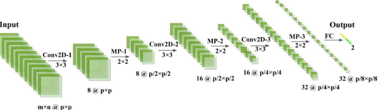
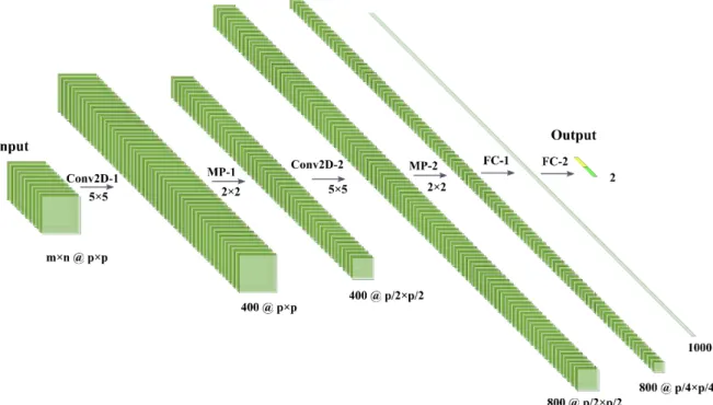
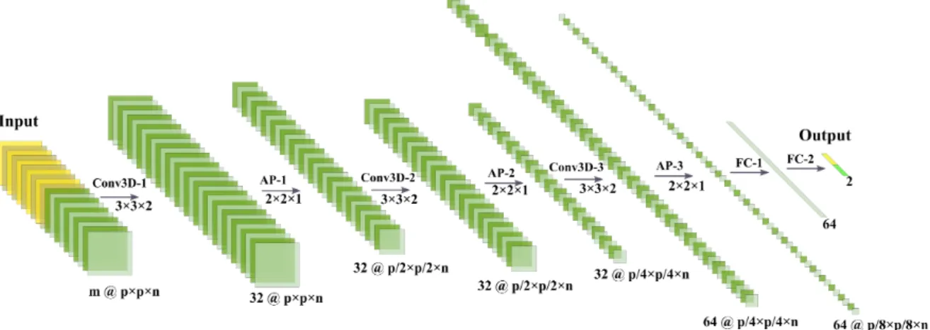
5.1 Architecture of ConvNet 2D-1 (Conv2D: 2D convolution, MP: Max-pooling, FC: Fully connected, m: number of channels, n: temporal depth, p: patch size) 28 5.2 Architecture of ConvNet 2D-2 (Conv2D: 2D convolution, MP: Max-pooling, FC: Fully connected, m: number of channels, n: temporal depth, p: patch size) 29 5.3 Architecture of ConvNet 2D-3 (Conv2D: 2D convolution, AP: Average-pooling, FC: Fully connected, m: number of channels, n: temporal depth, p: patch size) 29 5.4 Architecture of ConvNet 3D (Conv3D: 3D convolution, AP: Average-pooling, FC: Fully connected, m: number of channels, n: temporal depth, p: patch size) 30 5.5 General procedure of training classification networks (modified after [30]) . . 31
5.6 Architecture of 3D CNN. The detail architecture of each layer is listed in Table 5.4 36 5.7 General procedure of training yield estimation networks (modified after [31]) 37 6.1 Effect of varying input patch size . . . 41
6.2 Effect of the varying learning rate . . . 42
6.3 Effect of varying mini-batch size . . . 43
6.4 Significance of multi-temporal inputs . . . 43
6.5 (a) Ground truth-map of T45RUK tile in 2016; Rice maps generated by (b) SVM, (c) ConvNet 2D-1, (d) ConvNet 2D-2, (e) ConvNet 2D-3, and (f) ConvNet 3D (Blue and red circle represent exemplary areas used for discussing visual difference in model performance) . . . 48
6.6 Effect of variation in the ground-truth labels (model validation) . . . 49
6.7 Effect of dimensionality reduction (model evaluation) . . . 50
6.8 Variation in 3D CNN architecture by removing dimensionality reduction module 50 6.9 Contribution of auxiliary data in yield estimation (model validation) . . . 51
6.10 Effect of variation in the ground-truth labels (model evaluation) . . . 52
6.11 Effect of dimensionality reduction (model evaluation) . . . 52
6.12 Contribution of auxiliary data in yield estimation (model evaluation) . . . 53
6.13 (a) Ground-truth map of T45RUK tile; Maps showing estimated yields, gener-ated by (b) SVR, (c) 2D CNN, and (d) 3D CNN . . . 55
1.1
Contextual Background
Increasing population and climate change have imposed challenges in agriculture sector in terms of productivity, food security and sustainability [1]. The 2030 Agenda for Sustainable Development of the United Nations has explicitly defined that improving food security and ending hunger is one of their primary goals [2]. Timely and efficient agricultural monitoring is key to achieve this goal. In this context, remote sensing-based techniques are proven to be an effective technique to detect the regions with inadequate and poor crop growing conditions, to determine food-insecure areas and populations, and to monitor the development of crops [3]. Crop type mapping and yield estimation are essential for monitoring and decision-making process such as crop insurance, financial market fore-casting, and addressing food security issues. Multi-temporal and multispectral satellite images can be used to identify various types of crops and monitor their growth stages. Freely available multispectral satellite sensor imagery with coarse-to-medium spatial resolution such as Moderate Resolution Imaging Spectroradiometer (MODIS) and Landsat are the most frequently used data source in optical remote sensing [4][5][6]. However, the moderate spatial resolution of MODIS and lower temporal resolution of Landsat limits the accuracy in determining a detail crop extent. In this regard, the free availability of S2 imagery with high spatial and temporal resolution has unlocked extensive opportunities for agricultural applications that include crop mapping and monitoring as well.
As a part of the Copernicus European Earth Observation program, the S2 mission offers global coverage of terrestrial surfaces by means of high-resolution multi-spectral data [7]. In particular, the S2 mission includes two identical satellites (S2A launched on 23 June 2015 and S2B followed on 7 March 2017) that incorporate the Multi-Spectral Instrument (MSI). The S2 mission offers global coverage of land surfaces with innovative wide-swath of 290km, high spatial resolution ranging from 10m to 60m, high spectral resolution with 13 bands in the visible, near infra-red and shortwave infrared of the electromagnetic spectrum and high temporal resolution with 5 days revisit frequency. With these features, S2 imagery has potential to overcome the issues with coarse satellite imagery and costly data sources. Especially in developing countries, where crop monitoring process is very important but challenging at the same time due to the major problem of data availability, the S2 mission has an extensive scope to address these challenges and gaps. [8] also indi-cated that high-resolution crop type maps are not available globally and S2 imagery has
CHAPTER 1. INTRODUCTION
high potential to fill this breach of data availability and contribute to timely and accurate crop type maps.
In addition to high-quality remote sensing data, advanced and intelligent algorithms are essential for obtaining high accuracy in classification and yield estimation. Recently, deep learning algorithms such as CNN, Deep Neural Network (DNN) and Recurrent Neural network (RNN) have shown great potential in remote sensing applications such as land cover mapping, crop mapping tree species mapping and crop yield estimation. Traditional approaches for classification and regression tasks require feature engineering and field knowledge to extract features from images. While with deep learning algorithms, they have the ability to learn from multiple levels of representation [9]. These algorithms are proven to have outperformed the classical machine learning approaches In summary, the state-of-the-art on crop type classification and yield estimation has shifted from conven-tional machine learning algorithms to highly advanced deep learning classifiers, and from depending on only spectral features of single image to using both spectral and temporal information together for better accuracy [9].
1.2
Problem Statement and Motivation
Undoubtedly, a number of programs like Food and Agriculture Organization (FAO), Famine Early Warning System (FEWS), etc. exist that use satellite observations for crop monitoring on a regional to a global scale. Despite all these efforts, when it comes to a national or local scale actions, these monitoring systems do not effectively fulfill the need for crop monitoring and management [10]. Additionally, the use of traditional approaches for image classification is a time-consuming process that needs to be altered with the change in datasets and this hinders the timely availability of information, crucial for monitoring and decision-making process. Existing approaches for crop mapping and crop yield estimation mostly rely on survey data and other variables related to crop growth such as weather, precipitation and soil properties. These approaches are very successful in developed countries like in the United States, where adequate data with high quality are freely available [11]. However, in developing countries such as Nepal, complete and timely updated data are typically not available where the prediction of yields is most needed.
In Nepal, the national economy is dominated by agriculture. In a country where major part of the population is directly engaged in farming for their living, a high degree of spatial and temporal variability, traditional agricultural practices, climate change, and its vulnerability have imposed a serious challenge in effective and sustainable agriculture production [10]. In these circumstances, freely available S2 imagery motivates to conduct research and development in this field to address such challenges and make an effort
towards sustainable solutions. The fact that Deep Learning (DL) in agriculture has outper-formed the existing approaches and is growing popularity with its modern and promising technique, [12] also adds motivation to conduct this study.
1.3
Research Aims and Objectives
This work aims to support the crop monitoring process by investigating the viability of S2 data for rice crop classification and crop yield estimation in the Terai region of Nepal using a deep learning approach. To fulfill this aim, the following are the specific objectives:
• To review existing state-of-art deep learning algorithms for rice crop classification and yield estimation and select suitable architectures.
• To implement and optimize the performance of the chosen architectures.
• To evaluate the performance of classification and yield estimation models using performance metrics and validate their performance with reference to the existing works.
1.4
Methodology
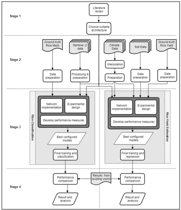
The structure of this thesis can be broadly organized into four stages namely; i) review and choice of network architecture; ii) dataset download/collection and preparation; iii) design, implementation, and analysis of network architectures, and iv) performance com-parison. The detailed structure of the overall methodology is shown in1.1.
In the first stage, a number of existing deep learning approaches used for crop classifica-tion and crop yield estimaclassifica-tion were reviewed. Considering the availability of the dataset and performance of deep learning algorithms, DNN was chosen as the core algorithm for addressing both the problems of classification and yield estimation. Besides this, Support Vector Machine (SVM) and Support Vector Regression (SVR), the mostly used classical machine learning algorithms for classification and regression problems, were used as baseline algorithms to compare the results of chosen CNN architectures against them.
Secondly, considering the rice crop phenology in the study area i.e., the Terai region of Nepal, S2 Level-1C (L1C) MSI images were downloaded for the years 2016-2018. These images were converted to atmospherically corrected S2 products, resampled to 20 m and further processed to feed the images to the CNN architecture for rice crop classification. In addition to these processed S2 images, ground truth-rice yield data, soil and climate data were collected and processed to 20 m in order to implement CNN architecture for yield estimation.
CHAPTER 1. INTRODUCTION
Figure 1.1: Overall methodology of the thesis
The third stage deals with the design, implementation, and analysis of the chosen CNN architectures. For classification purpose, three variations of 2D CNN and one 3D CNN architectures were implemented to inspect how the performance of the classifiers vary with the variations in the network architecture. For the second case which is the yield esti-mation process, two CNN architectures (2D and 3D CNN) were designed and employed. Several experimental designs were conducted so as to select the optimal values of the hyperparameters.
Finally, in the last phase, the performance of all the models using quantitative and qualita-tive approaches was evaluated. For a quantitaqualita-tive approach, two metrics namely overall accuracy and F1-score were used as measures to evaluate the performance of each classifi-cation approach. Similarly, RMSE was used for the performance evaluation of architectures
used for yield estimation. Additionally, visual inspection of classification and yield es-timation maps were used as a means for qualitative evaluation. Lastly, the optimized performance of the chosen architectures was validated with reference to the corresponding works from which these architectures were adopted to verify the usability of S2 data and the approach in developing countries like Nepal.
1.5
Contribution
In a broader picture, this study is one of the first studies (as per the author’s knowledge) that has introduced the use of S2 data for rice yield estimation including its classification by using a deep learning approach in developing countries with a case study in Nepal. The main contributions of this thesis consist of:
• Exploring the feasibility of using Sentinel 2-MSI data for crop classification and yield estimation in developing countries.
• Validating the suitability of S2 data combined with a deep learning approach for accurate rice crop management and sustainability with a case study of Nepal.
• Comparison of chosen CNN architectures and finding the best performing model in the study area.
• Introducing a variation in existing 3D CNN architecture [13] by removing the channel compression module to optimize its performance.
1.6
Thesis Organization
This thesis is divided into seven chapters. Chapter1introduces the contextual background of the thesis, states the problem and motivation behind the work, aims and objectives and highlights the contribution of the work. Chapter2reviews the related works on the existing methods for crop classification and yield estimation using remote sensing imagery and emphasizes on the state-of-art technologies with special focus on rice crop. Also, this chapter deals with the selected CNN architectures to be implemented to fulfill the objective of the study. Chapter3provides the theoretical background of the convolutional neural network architecture along with the baseline algorithms. Chapter4 familiarizes with the study area and presents the datasets used as input for CNN architectures. Chapter5
presents the methodological description of implementation, training, experimental settings and performance evaluation of chosen CNN-based classifiers for classification and yield estimation purposes. In Chapter6, the results of the experiments are shown, interpreted and discussed. Finally, the thesis ends with the conclusion and future directions of the work in Chapter7.
2
LITERATURE REVIEW
This chapter provides a comprehensive review of the existing state-of-art on crop clas-sification and yield estimation using remote sensing technology combined with deep learning techniques. The chapter is divided into two sections. The section2.1.1represents the traditional approaches used for crop mapping, especially rice crops. Thereafter, it deals with the deep learning approaches used in classification and finally explains the choice of network architectures and baseline. Similarly, the section2.2.1explains the traditional approaches used, deep learning algorithms, and choice of architecture and baseline for (rice) crop yield estimation.
2.1
Crop Classification
2.1.1 Traditional Approaches for Crop Classification
Remote sensing-based techniques are proven to be an effective technique for crop classi-fication and crop area estimation compared to traditional ground-based surveys which consume a lot of money and time. Time-series observations are essential to monitor the crop growth and multi-temporal remote sensing is an efficient source for this. Its classi-fication accuracy is higher than using mono-temporal images because it considers the crop information in different growth stages [4][14]. In multi-temporal remote sensing, various classification approaches and data sources have been used in past studies for crop mapping, especially rice crop. In terms of approaches for rice crop classification, they can be grouped into two types in general which are supervised and unsupervised classification [15]. Under supervised classification, knowledge-based [16] and phenology-based [17][18] approaches are the typical methods used.
In terms of data source, both optical and micro-wave based remote sensing have been used. In optical remote sensing, vegetation indices derived from images are used as a basis for rice crop classification. The commonly used indices are Normalized Difference Vegetation Index (NDVI), Enhanced Vegetation Index (EVI), and Land Surface Water Index (LSWI) [9][19]. Direct use of time series vegetation indices is effective for the crops that show distinct temporal characteristics [4][16]. A widely used approach of process-ing multi-temporal data is extractprocess-ing the phenological metrics which may improve the classification accuracy than using the original vegetation indices values. Freely available
multispectral satellite sensor imagery with a coarse-to-medium spatial resolution like MODIS and Landsat are the most frequently used data source in optical remote sensing [4][5][6][10]. However, the moderate spatial resolution of MODIS limits the accuracy in determining a crop extent and lower temporal resolution of Landsat images limits the usage of phenology-based crop classification and monitoring. A major limitation found in optical remote sensing is the influence of cloud and cloud shadows during the rice grow-ing season. Considergrow-ing this aspect, microwave-based remote sensgrow-ing has an advantage that it can work in all weather conditions. However, low temporal resolution and data cost have limited agricultural applications of Synthetic aperture radar (SAR) images.
Recently, the free availability of Sentinel imagery with the high spatial and temporal resolution has opened a broad opportunity for a wide range of pre-operational and oper-ational applications in the agricultural domain [20] resolving the issues with the coarse resolution of optical imagery and SAR. [21] has demonstrated Sentinel -1A and 2A’s remarkable potential for crop classification and suggested the integration of Sentinel-1A and 2A for high accuracy crop classification. However, with only Sentinel-1, [19] showed that high heterogeneity in pixel values of SAR image (Sentinel-S1) lowered the accuracy of land cover classification. It also concluded that although combining both sentinel-1 and sentinel-2 resulted in the highest accuracy, when multi-temporal data is available, it is not necessary to combine images from different sensors to obtain high accuracy results.
The use of traditional approaches for image classification is a time-consuming process that needs to be altered with the change in data sets and this hinders the timely avail-ability of information, crucial for monitoring and decision-making process. In addition to high-quality remote sensing data, advanced and intelligent classification algorithms are essential for obtaining high accuracy n classification provided that there are enough training data. Conventional classification methods such as SVM [22] Random Forest (RF) [23], and Decision Trees (DTL) [17][21][24][25][26] have been successfully applied in crop classification. While significant effort has been done to classify crops with these approaches, these algorithms require careful feature engineering and considerable domain knowledge to extract features from raw data [9][20].
2.1.2 Deep Learning Algorithms for Crop Classification
Recent developments in neural network methods through more layers and back-propagation optimization (deep neural network) have significantly increased the use of neural net-works that have been developed several years ago. DL in agriculture is new and gaining momentum recently. Based on the study of 40 recent (past four years) research papers that used DL in agriculture, [12] have concluded that DL has outperformed traditional approaches for image classification. DL is a deeper neural network that provides a hier-archical representation of the data which allows better learning capabilities in terms of capturing the full complexity of problems to be addressed. In this section, promising DL
CHAPTER 2. LITERATURE REVIEW
approaches used for crop classification are discussed.
One of the first works on crop classification using CNN classifiers to source multi-temporal satellite imagery was published by [20]. The study introduced one 2D CNN for spatial feature learning and one 1D CNN for spectral feature learning for crop classification which outperformed Multilayer Perceptrons (MLP) and RF classifier with overall classifi-cation accuracy of 94.6% achieved by 2D CNN. [27] employed a patch-based deep-learning CNN algorithm to extract rice crop using multi-temporal Landsat-like data, phenology data, and land-surface temperature. With multitemporal spectral bands as input, the 2D CNN achieved the overall classification accuracy of 91.23% demonstrating its better per-formance as compared to traditional machine learning classifiers, support vector machine and random forest. However, the paper did not consider the spatial pattern of the study area.
Authors in [27] highlighted that with a 2D CNN classifier, the extracted features in the third dimension (spectral or temporal) are averaged or collapsed to a scalar which results in inaccurate extraction of third-dimensional features. To overcome this problem of 2D CNN, the study proposed a 3D CNN with an active learning strategy for crop classifi-cation including rice using multi-temporal satellite data. When compared to a 2D CNN that shared the same architecture of 3D CNN except for the learned representation, 1.2% increase in overall accuracy was seen concluding that 3D CNN could be a better feature extractor for spatio-temporal remote sensing data. [28] used two deep neural networks: one-dimensional CNN (Conv1D) and Long Short Term Memory (LSTM) based RNN for multi-temporal crop classification using Landsat EVI time series. Three widely used non-deep-learning classifiers namely XGBoost, RF, and Support Vector Machine (SVM) were tested for comparison. The study demonstrated the lowest accuracy of LSTM with an overall accuracy of 82.41% among all classifiers and One-dimensional CNN (Conv1D) achieved the highest accuracy of 85.54% . The paper also attempted Three-dimensional CNN (Conv3D), which had the highest accuracy among all since it utilized pattern in both spatial and temporal dimensions, providing more scope of classification with 3D CNN for higher accuracy.
2.1.3 Choice of Network Architecture and Baseline
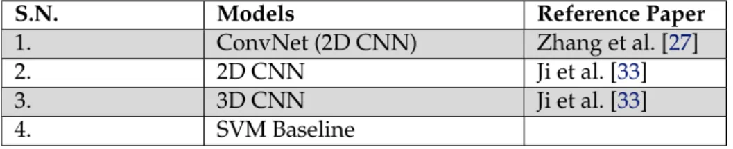
As this study focuses on assessing the performance of existing deep learning classifiers with S2 imagery in the study area, the choice of network architecture is based on the review of previous works as discussed in2.1.2. Exploring the trend of deep learning in rice crop classification, it is confirmed that CNN can perform better than other algorithms including LSTM for rice crop classification. Therefore, CNN is chosen as a core algorithm for rice crop mapping. [27] employed a simple patch-based ConvNet network with reference to the network architecture used by [29] for rice crop mapping and demonstrated its highest accuracy than the two full CNNs, a patch-based VGG-16 network [30] and a pixel-based
S.N. Models Reference Paper 1. ConvNet (2D CNN) Zhang et al. [27]
2. 2D CNN Ji et al. [33]
3. 3D CNN Ji et al. [33]
4. SVM Baseline
Table 2.1: List of chosen patch-based CNN architectures and baseline algorithm
Fully Convolutional Network (FCN) [31]. In the same year, [27] proposed a 3D CNN approach for rice crop classification which was based on widely used neural network architecture, VGGnet [32] where all 2D convolutions are replaced by 3D convolutions. The same architecture was employed to develop 2D CNN architecture and the performance evaluation of these two models demonstrated the higher classification accuracy of 3D CNN. Considering the higher accuracy of patch-based CNN than pixel-based, both the above-mentioned architectures were employed with an objective of evaluating and comparing the classification accuracy of the selected CNN architectures with S2 data in the study area.
An SVM classifier, well-known for high performance among the non-deep learning classi-fiers [27] and often established as a baseline model in the classification tasks is used as a baseline model in this study. In general, SVM with Radial Basis Function (RBF) kernel is considered to be a reasonable first choice to handle the case where the relationship between class labels and attributes is nonlinear. Having said that, [29] demonstrated higher accuracy of linear SVM in comparison to SVM with RBF kernel when the input dataset is huge. Therefore, taking this into, a linear SVM has been employed as a baseline model for comparing classification results. The network architectures and baseline algorithm chosen for rice classification purpose are summarized in Table2.1.
2.2
Crop Yield Estimation
2.2.1 Traditional Approaches for Crop Yield Estimation
Establishing models for estimating crop yield is very important but challenging at the same time in the remote sensing field. The classical approaches to predict or estimate crop yield include the use of manual surveys, Crop Simulation Model (CSM) or remote sensing data. Manual surveys require in-situ crop information, which are costly and difficult to scale to other regions. CSMs simulate the crop development, growth and yield through statistical, mechanistic or functional models as functions of soil, weather and management practices [34]. However, these models require large datasets for model calibration and therefore may not be applicable for developing countries where data is scarce and sparse. Many studies have shown the use of remote sensing technology to estimate the crop production by employing statistical methods such as regression model. [35] employed a piecewise linear regression method with a breakpoint to predict corn and soybean yields using NDVI, surface temperature, precipitation, and soil moisture. [36] used a
CHAPTER 2. LITERATURE REVIEW
stepwise regression method for estimating winter wheat yields using MODIS NDVI data. [37] estimated crop yields with the prediction error of about 10% in the US Midwest by employing Ordinary Least Squares (OLS) regression model using time-series MODIS products and climate dataset. In summary, the classical approach for crop yield estimation is mostly based on the multivariate regression analysis using the relationship between crop yields and agro-environmental variables like vegetation indices, climatic variables, and soil moisture. These approaches have compactly summarized the information related to vegetation growth with the use of vegetation indices which depend on a smaller number of available bands, usually two. But the bands which are ignored with this approach could have additional important information to predict the yield with more accuracy.
With advances in Machine Learning (ML), researchers have applied machine learning algorithms to remote sensing imagery for crop yield prediction. [38] introduced the use of Artificial Neural Network (ANN) through a back-propagation algorithm in forecasting winter wheat crop yield using remote sensing data to overcome the problem that existed in using traditional statistical algorithms (especially regression models) due to nonlinear character of agricultural ecosystems. The study demonstrated high accuracy of ANN compared to results from a multi-regression linear model (MR model). The commonly used machine learning techniques include SVM, DT, and MLP [39]. These techniques have contributed to improving the accuracy of crop prediction. However, these approaches require feature engineering. On the other hand, with deep learning algorithms, they auto-matically learn the relevant features from the raw data effectively.
2.2.2 Deep learning in Crop Yield Estimation
One of the first works on employing a deep learning approach for crop yield estimation was done by [40]. The study employed a Caffe-based deep learning regression model with satellite, climate and environmental data to estimate corn crop yield at county-level in the United States. The proposed architecture achieved an RMSE of 6.298 outperforming the performance of SVR. [11] introduced a new dimensionality reduction technique i.e. treating raw images as histogram of pixel counts under the assumption of permutation variance and trained deep learning architectures CNN and LSTM on these histograms to predict county-level soybean yields in U.S. To address spatial and temporal dependencies across data points, the paper proposed the use of linear Gaussian Process layer on the top of these neural network architectures. To compare with prior works, the inputs datasets used for this study are long-term (2003-2015) MODIS satellite-based surface reflectance, LST and land cover data. The baseline methods used to compare the results were ridge regression, decision trees, and a DNN with 3 hidden layers. The results demonstrated that CNN and LSTM approaches outperformed the other competing techniques used as baselines. Also, prediction was improved by addition of linear GP resulting in 30% reduction of RMSE from baselines.
The location invariant assumption by [11] discards the spatial information of satellite imagery which can also be crucial information for crop yield estimation. To overcome this, [13] introduced a 3D CNN approach that considers both spatial and temporal features for yield prediction. Firstly, the paper replicated the Histogram CNN approach of [11] with the same input dataset and set this as a baseline for their novel approach, 3D CNN. Considering the computational cost, a channel compression model was applied to lessen the channel dimension from 10 to 3. Thereafter a 3D CNN was stacked to the model. The proposed 3D CNN architecture outperformed the replicated Histogram CNN and non-deep learning classifiers used as baselines [11] with an average RMSE of 5.27 bushels per acre (around 355 kg/ha). Continuing to the same data, [41] proposed a novel approach of deep CNN-LSTM model for end-of-season and in-season soybean yield prediction. The proposed network consisted of 2D CNN followed by LSTM where CNN learns the spatial features and LSTM is used to learn the temporal features extracted by CNN. The proposed model achieved reduced RMSE of average 329.53 kg/ha which was better than CNN and LSTM models.
Recently, [42] applied a CNN model to predict crop yield using NDVI and Red, Blue, Green (RGB) images acquired from Unmanned Aerial Vehicle (UAV). The result showed the better performance of CNN architecture with RGB data. [43] proposed a novel CNN architecture which used two separate branches to process RGB and multispectral images from UAV to predict rice yield in Southern China. The resulting accuracy outperformed the traditional vegetation index-based regression model. The study also highlighted that unlike the vegetation index-based regression model, the performance of CNN for yield estimation at the maturing stage is much better and more robust.
2.2.3 Choice of Network Architecture and Baseline
Based on the related literature discussed in section2.2.2, CNN and LSTM are mostly used deep learning algorithms to address the problem for crop yield prediction with high accu-racy. On the one hand, when these algorithms were used separately, [11] demonstrated that CNN achieved higher accuracy than LSTM. On the other hand, the combined model, CNN-LST performed relatively better [41]. However, these experiments were conducted using a long-term dataset with a high temporal dimension. The limited temporal dimen-sion of the dataset in this study limits the use of the LSTM model. Therefore, for rice crop yield estimation also, CNN is chosen as a core algorithm. Exploring the performance of various architectures of CNN in the previous studies,3DCNNproposed by[13]achieved the highest accuracy to date and is therefore chosen as the base architecture for this study. Similar to SVM,SVRis commonly used to perform yield prediction and will be used as a baseline to compare the performance of 3D CNN against it.
3
THEORETICAL BACKGROUND
This chapter is meant to serve as the theoretical foundation of the concepts used in the thesis. The first section presents a brief explanation about the classical machine learning approaches which have been selected as baselines for the crop classification and yield estimation tasks. The second section starts with some limelight on deep learning and neural networks which is followed by background concepts of CNN in detail.3.1
Classical Machine Learning Approach
This section gives a brief theoretical overview of the classical machine learning algo-rithms namely SVM and SVR used as baselines for comparing the performance of CNN algorithms used for rice crop classification and yield estimation respectively.
3.1.1 Support Vector Machine
SVM, as proposed in statistical learning theory [44], is known to be an effective kernel-based classification algorithm that is kernel-based on statistical learning theorem. The main objective of SVM is to find the optimal linearly separating hyperplane which maximizes the margin. The key idea behind kernel tricks is to map data in to a higher-dimensional space so that different groups or classes can be linearly separable [45]. Mathematically, the optimization problem for support vector machine can be formulated as,
min w,b 1 2kwk 2 s.t. yi wTxi+b ≥1 ,i=1, ...,m (3.1)
where(w,b)defines a hyperplane that separates all the training data into the two labeled classes,xiare the input data andyi are labels. This is a quadratic optimization problem subject to linear constraints. The objective is a convex function with a unique minimum. For linearly non-separable classes, non-linear decision boundaries can be constructed using for instance, a radial basis function (RBF) [16][46].
3.1.2 Support Vector Regression
A regression model estimates a continuous-valued multivariate function. SVR is an ex-tension of SVM algorithm which was introduced for regression scenarios to predict the numerical property values [47]. In case of SVM an optimal hyperplane is generated for class label prediction, on the other hand in SVR, a different function is derived based on training data to predict numerical values. SVR has proven to be an effective tool for estimating the real-value function.
3.2
Artificial Neural Networks and Deep Learning
ANN and DL are state-of-art technology that is providing the best solution to existing machine learning algorithms. ANN is a type of machine learning and is inspired by the biological nervous system and consists of interconnected neurons that work in a distributed fashion to learn from input in order to optimize its final output [48]. DL also belongs to a broader family of machine learning and is inspired by ANN. Although DL is similar to ANN, it constitutes a deeper neural network that allows better learning capabilities to capture the full complexity of the considered data or phenomenon [49]. Deep learning architectures such as deep neural networks, unsupervised pre-trained networks, recurrent neural networks, recursive neural networks and CNN have been successfully applied to diverse fields including computer vision, speech recognition, audio recognition, natural language processing, medical image analysis, and so on with high accuracy and have proven to be superior than the classical machine learning algorithms. Since we have chosen CNN as a core algorithm for this study, the following subsections deal with the detailed architecture of CNN.
3.2.1 Convolutional Neural Networks
CNNs are biologically inspired feed-forward neural networks that extend the classical artificial neural network approach by adding multiple convolutional layers and filters that allow representing the input data in a hierarchical way [50]. CNN exhibits high performance in image processing tasks, thereby positioning itself as the current state-of-the-art of image classification methods. Traditional neural networks (deep or shallow ones) which are characterized by 1D architectures are composed of (Fully Connected (FC)) layers. Whereas in CNN, hidden activation is calculated by multiplying small local inputs against weights and exploits spatially local association by applying a local pattern of connectivity between adjacent layer neurons. The weights are then shared across the entire input space. The output volume of CNN is composed of feature maps which are then used as input to the next layer. The basic concepts employed in CNN are explained in the following subsections:
CHAPTER 3. THEORETICAL BACKGROUND
3.2.1.1 Basic Architecture
The basic architecture of CNN consists of alternatively stacked convolutions blocks and pooling layers followed by one or more fully connected layers. The convolutional blocks are usually composed of convolutional layers followed by batch normalization layers and nonlinear activation functions. The convolution and pooling layers act as feature extractors from the input images. At last, the fully connected layer, after a series of convolution and pooling, gives the class score of each pixel through the network in a feed-forward manner. A detailed explanation is presented here.
Convolutional layer
The convolutional layer is the core building block of the convolutional network that consists of filters (also termed as kernels) which are applied over the image to extract different features learned by the network. Convolution layer computes the output of neurons that are connected to the local regions in the input by conducting dot product between their weights and biases and a specific region to which they are related in the input range [48]. Mathematically,
xl+1 = f(Wlxl+bl), (3.2)
wherexl+1is the output with n feature maps of thelth convolution layer,Wl is weight matrix defined by the filter bank with kernel sizeN×Nandbl is the bias of thelth convo-lution layer, and f()being the nonlinear activation function.
In this study, the input is taken from multispectral-temporal images. The basic way is to treat each channel independently and generate a uniform-sized image patch around the same images. Let us suppose a multispectral image X ∈ R(M×D×H) where M, D, H are the spectral bands, width, and height respectively. The pixel x(i,j)of X (with i = 1, 2, . . . ,Dand j = 1, 2, . . . ,H) can be defined as the spectral vector x(i,j) ∈ RM =
[x1(i,j),x2(i,j), ...,xM(i,j)]. Let us define a neighboring region (image patch)q(i,j)∈ R(p×p) around x(i,j), composed of pixels from ((i−(p2),j−(p2)), ((i+ (p2),j−(p2)),((i− (p2),j+ (p2)),((i+ (p2),j+ (p2)). With q taking account of spectral information, it can be redefined asq(i,j)∈R(M×p×p). The convolution layer takes ap×pimage patch withM channels centered at a pixel x(i,j)and two-dimensional filter kernelN×Nwithknumber of filter. Letyk(i,j)be pixel value at output feature map andwk(r,s)be weight value at
(r,s)atkthfilter. Then mathematically, the convolution process is defined as [33],
yk(i,j) = M
∑
m=0 ( N−1∑
r=0 N−1∑
s=0 wk(r,s)xm(i,j) (i+r,j+s) ) +bk, (3.3)The convolution operation in a normal image down-samples the output image size by an amount that depends on the filter size. To avoid this,paddingis used which essentially preserves the original input image size. Padding is simply a process of adding layers of
zeroes to the input images. There are two types of padding namelyvalidpadding which implies no padding at all andsamepadding which means the output feature map has the same dimension as the input image.
Batch normalization is a process to reduce the co-variance shift by normalizing the layer’s inputs over a mini-batch. It enables independent learning process in each layer and regularizes and accelerates the training process. Mathematically, it is defined as:
BN(x) =px−E(x)
Var(x) +ε
γ+β, (3.4)
where E is expectation operator,γandβare learn-able parameter vectors, respectively,
andεis a parameter for numerical stability. This layer makes the hyperparameter search
much easier and make the neural network more robust and enable easier training of the deep network.
Activation functions are used to embed non-linearity into the neural network thereby enabling the neural network to learn nonlinear representations. Activation function can be expressed as: Z(yk(i,j)) = f K
∑
k=1 xk(i,j)wk+bk ! , (3.5)where f()is a non- linear function. There are varieties of activation functions such as sigmoid function, Tanh, Rectified Linear Unit (ReLU) [51] and Exponential Linear Unit (ELU). Sigmoid and Tanh tend to saturate when initialized weights are too high and give rise to a problem of vanishing gradient if gradient tends to zero. ReLU solves this problem by thresholding the negative inputs to zero and passing the positive inputs unchanged [52]. ReLU is proven to be computationally efficient and effective for convergence and is defined as
A(yk(i,j)) =max(0,Z(yk(i,j))), (3.6)
Pooling layer
The pooling layer is a sub-sampling operation along the spatial dimensions of feature maps, typically applied after a convolution layer, which does some spatial invariance [48]. Usually, in pooling, some predefined functions (e.g. maximum, average, etc.) are applied to summarize the signal and spatially preserving discriminant information.Max-pooling is a non-linear sub-sampling operation whereasaverage pooling, on the other hand, can be thought of as a low-pass (averaging) filter followed by sub-sampling. The pooling region can be overlapped or non-overlapped and in the latter case, the more information is lost. The output of max pooling for a local region of dimensionk×kcan be mathematically defined simply as,
CHAPTER 3. THEORETICAL BACKGROUND
yk ip,jp= max
0≤ip≤np−1,0≤jp≤np−1
A(yk(i,j)), (3.7)
The parameters to be defined by the user are the size of the window and stride (number of steps between the consecutive convolutions). After pooling layer the output is a 3D cube composed of one 2D map per filter with a reduced spatial dimension.
Fully Connected Layer
In a typical CNN architecture, the FC layer is usually placed at the end of the network after several convolutions and pooling layers. FC layer takes the output of the previous layers, flattens them and turns them inton (number of classes)dimensional vector that can be input to the next stage. Each number in thisn-dimensional vector represents the probability that a certain feature belongs to one of the predefined classes. If there are multiple FC layers, the initial layers take the outputs from previous layers and apply weight to predict the correct label and the last FC layer gives the final probabilities for each label. In a FC layer, neurons have connections to all the activations in the preceding layers which is analogous to the output layer of MLP [48].
Classification layer
The output from the fully connected layer is fed to the classifier layer to calculate the probabilistic output of each class. The classification layer calculates the cross-entropy loss for multi-class classification problems with mutually exclusive classes. The most common classifier for multi-class classification is softmax [53] and for a binary classification prob-lem, it reduces to be a logistic regression. A Softmax function limits the output into the range of [0 1] which allows being interpreted as a probability.
Let us assumenk×nk×Uis the form of the output of the CNN, where U is the number of channels of output image patch m.X = [x1,x2, ... ,xu]T represent the pixel value in the output of fully connected layer and softmax function is used to generate a vector K = [k1,k2, ...ku]T of real values in the range of [0,1] which represents a categorical distribution . The equation 3.8 shows how softmax function predicts the probabilities of jth class given the sample vectorX.
Kw,b= exp xwj ∑U u=1exp(xwu) , (3.8) Regression Layer
For regression problems, the classification layer of CNN is replaced by the regression layer. A regression layer returns the regression output of the neural network and computes the half-mean-squared-loss for regression problems. Mathematically,
loss = 1
2 nknkU
wherenk×nk×Uis the dimension of final output of the CNN;yibeing target output and xibeing network prediction for responsei.
Regularization
Over-fitting is a serious problem in the deep learning networks where networks are powerful enough to fit itself to the training data resulting in large gap between the training and test errors. Regularization techniques are used to prevent overfitting the data (to reduce high variance) in the network and reduce its generalization error. There are several regularization techniques such as L2 and L1 regularization, dropout, and early stopping. L1 regularization makes the model sparse and that only contributes to regularize the model to less extent and therefore is not used often. L2 regularization (also known as weight decay) is one of the most commonly used regularization techniques. It basically minimizes the sum of the square of the differences (S)between the target valueyi,j and the estimated values f xi,j
: S= N
∑
i=1 N∑
j=1 yi,j− f xi,j 2 , (3.10)Dropout is another powerful regularization technique that randomly knocks out units in the network resulting in a smaller network. The smaller network seems to have a regularization effect. Early stopping is a simple yet effective regularization technique while training the neural networks. It is used to stop the training of the neural network (with training dataset) at a point when the performance on a validation dataset starts to degrade.
3.2.1.2 Training
The training process of CNN can be divided into three major steps: forward computation, loss optimization, and back-propagation and parameter updating.
Forward Computation
Firstly, the input is fed through the neural network architecture consisting of a series of convolution, pooling and fully connected layers as explained in the previous subsec-tion. The network outputs the predicted labels or values depending upon the network architecture (classification or regression).
Loss Optimization
Secondly, the output of the network needs to be optimized by adjusting the values of parameters such as weights and bias, that are being learned by the network. The optimiza-tion problem defines the uncertainty in determining the optimal set of parameters which is quantified by the loss function. In the case of softmax classifier, the cross-entropy loss
CHAPTER 3. THEORETICAL BACKGROUND
for each vector is computed as negative log-likelihood of the training dataset N under the model. L(W,b) =−1 N N
∑
i=1 yilogKw,bxi, (3.11)whereyirepresents a possible class andxiis the data ofiinstance,W is the weights, and Nrepresents a total number of instances.
Back Propagation
Finally, training of the network must be done for extracting the parameters that minimize the loss. The network tries to reduce this error by changing the weights of neurons in every iteration through the backpropagation mechanism. Several optimization algorithms exist to make the training process faster such as Stochastic Gradient Descent (SGD) with momentum, Adaptive Gradient (AdaGrad), Root Mean Square Propagation (RMSProp), and Adaptive Moment Estimation (Adam) among which we will discuss in brief about two algorithms which have been used for this study namely SGD with momentum and Adam.
Stochastic Gradient Descent with Momentum:
SGD with momentum basically calculates the exponentially weighted average of the gradients and consider that gradient to update the weights. It is used for faster convergence of the loss function.α(learning rate) andβ(momentum) are the two hyperparameters
which control the exponentially weighted average. In practice, the most common value ofβis 0.9. Mathematically, the SGD method with momentum can be described by the
following:
W(n+1)=W(n)−∆W(n+1), (3.12) whereW(n)andW(n+1)denote the old parameters and new parameters respectively and ∆W(n+1)represents the increment in the current iteration which is the combination of old parameter, gradient and historical increment:
∆W(n+1)= α dwW(n)+ ∂L(Wb) ∂W(n) +β∆W(n), (3.13)
where L(W,b) is the loss function,αis the learning rate for step length control anddwand
βdenote the weight decay and momentum
respectively-Adam optimization algorithm:
Adaptive Moment Estimation (Adam), introduced by [54], is also based on mini-batch gra-dient descent and computes adaptive learning rates for each parameter. It is an extension to stochastic gradient descent which basically takes momentum and RMSprop and puts them together. The algorithm specifically calculates an exponential moving average of the
gradient and the square gradient, and theβ1andβ2parameters control the decay rates of these moving averages.
mt = β1mt−1+ (1−β1)g1, (3.14)
ϑt = β2ϑt−1+ (1−β2)g2t, (3.15) wheremt andϑtare estimates of the first moment and second moment of the gradient respectively. In practice, the default value forβ1andβ2, 0.9 and 0.999 are most commonly in use. The bias corrected first, and second moment estimates are then computed as:
c
mt = mt
1−βt1 , (3.16)
ϑt =β2ϑt−1+ (1−β2)g2t , (3.17) Finally, these biased corrected moment estimates are used to update parameters using adam update rule:
θt+1 =θt− α q b ϑt+e c mt, (3.18)
3.2.1.3 Parameters and Hyperparameters
Parameters are the variables that model updates during the back-propagation phase. Weights and biases are the core parameters of deep neural networks. Whereas, hyperpa-rameters are the specific “higher-level” properties of the models which should be fixed prior to the training process. The value of these parameters cannot be directly learned from the regular training process of the model. Hyperparameters need to be tuned for each problem because the best model hyperparameters for one dataset will not be best for all datasets. The process of finding the combination of hyperparameter values for a model that performs the best as measured on a validation dataset is termed as hyperparameter tuning (also known as hyperparameter optimization). Hyperparameters can be divided into two types: hyperparameters that determine the network structure such as kernel size, stride, padding hidden layers, and activation function and hyperparameters that determined the network training process such as learning rate, batch size, number of epochs, regularization techniques and so on. Here, we will focus on the second type and a brief explanation of some influential hyperparameters is presented in the following subsection:
Learning Rate:
Learning rate simply means how fast a network learns. It quantifies the learning process of a model that can be used to optimize its capacity. Choosing a learning rate is challenging as a value too small causes the model to take much time to converge, whereas a value too
CHAPTER 3. THEORETICAL BACKGROUND
large cause model to diverge and loss might fluctuate indefinitely [55]. A general approach used by many of the previous works was to start out with a high learning rate and lower it as the training goes on. One point to note is that the learning rate is very dependent on the network architecture. The updating of the learning rate can be formulated as:
αt=α0∀t <τ (3.19)
αt =α0tdt, (3.20)
whereα0andαtare initial learning rate and learning rate at iteration t; d is decay parameter.
τandαare set up to adapt depending upon the present thresholds of the loss function.
Mini-batch size:
When the mini-batch size is equal the size of the input, then it is known as batch gradient descent (too long per iteration) and when the mini-batch size is equal to the one (noisy and doesn’t converge), then it is known as Stochastic gradient descent. In practice, the mini-batch size of an appropriate value between 1 and the max value (not so big or small) is chosen which gives the fastest learning.
Number of epochs:
It is a hyperparameter that controls the number of complete passes through the training dataset. The weights are updated after each epoch and hence produce better results. However, using many epochs might over fit the training process and this is when early stopping can be used which prevents the overfitting of the model.
3.2.2 3D Convolutional Neural Network
In 2D CNN, all the spatio-temporal images are stacked together as the input and after the first convolution, the temporal information is collapsed completely [33]. To prevent this, 3D CNN uses 3D convolutions that apply 3-dimensional filters to the dataset resulting in a 3-dimensional volume space. In 3D CNN, the 3D convolution pooling operations are performed spatio-temporally which shows its ability to model the temporal information better than 2D CNN [56]. 3D CNN is not only limited to event detection in videos or 3D medical imaging but also applied to 2D input space such as images.
The convolution in equation3.3for 2D convolution can be modified to extract and reserve the dynamic features through consecutive periods and can be written as:
yk(i,j,h) = M
∑
n=0 ( N−1∑
r=0 N−1∑
s=0 N−1∑
t=0 wk(r,s,t)xm(i,j,h) (i+r,j+s,h+t) ) +bk, (3.21)wherexm(i,j,h)is input pixel at input image or feature map andym(i,j,h) are input and output pixel value at output feature map,wk(r,s,t)be weight value at(r,s,t)atkth filter andbis the bias.
USED
This chapter introduces the study area in the first part and provides the background information behind the motivation of conducting the study in this area. The second part of this chapter is focused on explaining the datasets that have been considered for the implementation of the designed algorithms.
4.1
Study Area
Figure 4.1: Study area with elevation profile and sentinel tiles
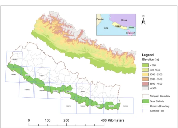
This study is based on 20 districts of the Terai region of Nepal that comprise a lowland in southern Nepal (Figure4.1). Nepal is a small landlocked country with an area of 147,181 km2 stretching from 26◦ 22’ to 30◦ 27’ N and from 80◦ 04’ to 88◦ 12’ E. The principal
CHAPTER 4. STUDY AREA AND DATASETS USED
economic activity of Nepal is agriculture, which constitutes about one-third of the Gross Domestic Product (GDP) and employs nearly three-fourth of the labor force [57]. Of the total basic crop production, paddy production is the highest in the country sharing 20.75% of the total GDP from agriculture [58]. Even though the Terai region covers just 23.1% of the total area of the country, it comprises 49% of the total agricultural land. The rice production is mainly located on the Terai districts which contributes about 70% of the total rice production of the country. As a result, the domestic food security of Nepal is critically reliant on the sustainability of the cereal production system of this region. According to CBS (2011), 84% of the farm households in the Terai region are actively engaged in rice production. However, the growth rate of the agricultural sector of Nepal is too low to meet the growing food demand of the increasing population, indicating that public and private investments in the agricultural Research and Development (R&D) sector would increase cereal productivity in Nepal [59].
4.2
Datasets used
4.2.1 S2 Level-1C products S2
Bands
Band Names Central Wave-length (nm)
Bandwidth (nm)
Spatial Reso-lution (m)
Band 1 Coastal Aerosol 443 20 60
Band 2 Blue 490 65 10
Band 3 Green 560 35 10
Band 4 Red 665 30 10
Band 5 Vegetation Red Edge
705 15 20
Band 6 Vegetation Red Edge
740 15 20
Band 7 Vegetation Red Edge
783 20 20
Band 8a Near-Infrared 842 115 10
Band 8b Vegetation Red Edge
865 20 20
Band 9 Water Vapour 945 20 60
Band 10 SWIR-Cirrus 1375 30 60
Band 11 SWIR 1610 90 20
Band12 SWIR 2190 180 20
Table 4.1: S2 spectral bands definition, Source: [60]
The key phases of the rice crop cycle, i.e. start of the season, the peak of season and end of the season, in the Terai region of Nepal correspond to July, September, and mid-November respectively [10]. Therefore, the L1C products during these key periods were downloaded for the years 2016-2018. In case of missing or corrupted images, products within a week before or after the mid-month were downloaded. 14 sentinel tiles (zone
44 and 45) in total covered the study area as shown in (Figure4.1. Therefore, a total of 126 L1C products were downloaded. The S2 L1C products are provided free from ESA’s Scientific Data Hub (SDH) in Standard Archive Format for Europe Format (SAFE) files. S2 sensor provides a total of 13 spectral bands with a high spatial resolution ranging from 10m to 60m (Table4.1). Among these spectral bands, the classical RGB and Near Infrared (NIR) bands with 10m spatial resolution are dedicated to land applications. The 20m bands which 4 narrow bands in the vegetation red edge spectral domain and 2 Shortwave Infrared (SWIR) large bands, which are used for snow/ice/cloud detection and moisture stress assessment. The remaining bands at 60m are dedicated to atmospheric correction and cirrus detection.
Both satellites have a wide-swath of 290 km and fly in the same orbit phased at 180◦ providing a high temporal resolution with a revisit frequency of 5 days for S2 operational data products [61]. S2 L1C and Level-2A (L2A) products are provided in tiles, also called granules, which consist of 100×100 km2ortho-images in UTM/WGS84 projection. The Universal Transverse Mercator (UTM)system divides the Earth’s surface into 60 zones. Each UTM has a vertical width of 6◦of longitude and a horizontal width of 8◦of latitude. On the one hand, L1C products are top-of-atmosphere Top-of-Atmosphere (TOA) radiance images which are radiometrically and geometrically corrected as well as orthorectified using the global Digital Elevation Model (DEM). On the other hand, L2A products provide Bottom-of-Atmosphere (BOA) reflectance images derived from the corresponding L1C products. For this study, L1C products are considered since L2A products are only available from the end of 2018 for regions outside Europe.
Sentinel Data Processing
A total of 126 S2 L1C products were converted to atmospherically corrected L2A products using the Sen2Cor processor which is based on algorithms proposed in the Atmospheric/-Topographic Correction for Satellite Imagery (ATCOR) [62]. Sen2Cor is supported by ESA as a third-party plugin for the S2 toolbox (standalone version). It runs in the ESA Sentinel Application Platform (SNAP) or from the command line. Additionally, topographic cor-rection with a 90m digital elevation database from CGIAR-CSI (http://www.cgiar-csi.org) and cirrus corrections were applied [63]. Topographic correction here is purely radiometric and does not change the image geometry. However, the resulting products showed that cirrus correction with Sen2Cor was not effective. Moreover, the products had significant cloud and cloud shadows. So, to deal with these problems, cloud mask data available with L1C products that specifies the percentage of cloudy pixels and cirrus pixels, was considered during the post processing of L2A products. The whole process was performed in batch processing from the command prompt. The whole process was performed in batch processing from the command prompt.
CHAPTER 4. STUDY AREA AND DATASETS USED
Figure 4.2: S2 L2A data processing chain in SNAP Graph Builder
After generating L2C products, the next step was to calculate the NDVI. This process involves a chain of data processing tools as shown in Figure4.2. Taking into account the total size of the considered products (over 100 GB) and the high computational cost of managing such data volume, we decided to store the final products in 20 m instead of 10 m. Therefore, the resulting L2A products were all resampled to 20 m. Thereafter, a spatial subset was applied to clip the images to the extent of the study area. Among the 13 spectral bands of S2, the three bands with 60 m resolution (B01, B09, and B10) are dedicated to atmospheric correction and cirrus detection. These bands are typically not considered in crop classification tasks [7] so, they were excluded from the output data. As a result, 4 bands resampled to 20 m (B02-B04 and B8a) and 6 bands with a nominal spatial resolution of 20 m (B05-B07, B8b, B11, and B12) were concatenated for the considered data processing chain. Bands B04 and B8a bands represent the red and NIR channels respectively (see Table4.1) and were used to calculate the NDVI using BandMaths tool as follows:
NDV I = (ρnir−ρred)
(ρnir+ρred), (4.1)
where ρnir represents the reflectance of the near-infrared band and ρred represents the reflectance of the red band. NDVI is the most commonly used indicator to monitor vegetation health and classifies vegetation extent. As a result, the resulting NDVI product was also merged as an additional band to the final product in the GeoTIFF file format. Considering the presence of significant cloud coverage in the images, cloud mask data available with L1C products was also concatenated with the bands. An option is to use these cloud masks to filter the images when training the corresponding crop classification models. Due to the high cloud cover in June (heavy monsoon period), only the images of September and November have been considered for the classification and yield estimation experiments reported in this work.
4.2.2 Ground-Truth Data: Rice Mask
Considering the major limitation on the availability of a real high-resolution ground-truth map of rice crops in the study area, the rice mapping approach adopted by [10] was utilized in the long-term period 2006-2014 to generate the final ground-truth rice map considered in this work. Specifically, this procedure considers the most optimistic rice map based on the classification conducted using MODIS data. The resulting rice map has also been filtered by using the land cover mask produced by [22] in order to ensure that the ground-truth maps do not include non-agricultural areas if any. Finally, the output
![Table 4.1: S2 spectral bands definition, Source: [60]](https://thumb-us.123doks.com/thumbv2/123dok_us/9951714.2487841/34.892.167.768.588.984/table-s-spectral-bands-definition-source.webp)


![Figure 5.5: General procedure of training classification networks (modified after [30])](https://thumb-us.123doks.com/thumbv2/123dok_us/9951714.2487841/43.892.151.800.511.736/figure-general-procedure-training-classification-networks-modified.webp)
