Multilabel Structured Output Learning with Random
Spanning Trees of Max-Margin Markov Networks
Mario Marchand
D´epartement d’informatique et g´enie logiciel Universit´e Laval
Qu´ebec (QC), Canada
Hongyu Su
Helsinki Institute for Information Technology Dept of Information and Computer Science
Aalto University, Finland [email protected]
Emilie Morvant∗ LaHC, UMR CNRS 5516 Univ. of St-Etienne, France
Juho Rousu
Helsinki Institute for Information Technology Dept of Information and Computer Science
Aalto University, Finland [email protected]
John Shawe-Taylor Department of Computer Science
University College London London, UK
Abstract
We show that the usual score function for conditional Markov networks can be written as the expectation over the scores of their spanning trees. We also show that a small random sample of these output trees can attain a significant fraction of the margin obtained by the complete graph and we provide conditions under which we can perform tractable inference. The experimental results confirm that practical learning is scalable to realistic datasets using this approach.
1
Introduction
Finding an hyperplane that minimizes the number of misclassifications isN P-hard. But the support vector machine (SVM) substitutes the hinge for the discrete loss and, modulo a margin assumption, can nonetheless efficiently find a hyperplane with a guarantee of good generalization. This paper investigates whether the problem of inference over a complete graph in structured output prediction can be avoided in an analogous way based on a margin assumption.
We first show that the score function for the complete output graph can be expressed as the expec-tation over the scores of random spanning trees. A sampling result then shows that a small random sample of these output trees can attain a significant fraction of the margin obtained by the complete graph. Together with a generalization bound for the sample of trees, this shows that we can obtain good generalization using the average scores of a sample of trees in place of the complete graph. We have thus reduced the intractable inference problem to a convex optimization not dissimilar to a SVM. The key inference problem to enable learning with this ensemble now becomes finding the maximum violator for the (finite sample) average tree score. We then provide the conditions under which the inference problem is tractable. Experimental results confirm this prediction and show that
∗
practical learning is scalable to realistic datasets using this approach with the resulting classification accuracy enhanced over more naive ways of training the individual tree score functions.
The paper aims at exploring the potential ramifications of the random spanning tree observation both theoretically and practically. As such, we think that we have laid the foundations for a fruitful approach to tackle the intractability of inference in a number of scenarios. Other attractive features are that we do not require knowledge of the output graph’s structure, that the optimization is convex, and that the accuracy of the optimization can be traded against computation. Our approach is firmly rooted in the maximum margin Markov network analysis [1]. Other ways to address the intractability of loopy graph inference have included using approximate MAP inference with tree-based and LP relaxations [2], semi-definite programming convex relaxations [3], special cases of graph classes for which inference is efficient [4], use of random tree score functions in heuristic combinations [5]. Our work is not based on any of these approaches, despite superficial resemblances to, e.g., the trees in tree-based relaxations and the use of random trees in [5]. We believe it represents a distinct approach to a fundamental problem of learning and, as such, is worthy of further investigation.
2
Definitions and Assumptions
We consider supervised learning problems where the input spaceXis arbitrary and the output space Y consists of the set of all`-dimensional multilabel vectors(y1, . . . , y`)
def
= ywhere each yi ∈
{1, . . . , ri}for some finite positive integerri. Each example(x,y)∈ X ×Yis mapped to a joint
feature vectorφφφ(x,y). Given a weight vectorwin the space of joint feature vectors, the predicted outputyw(x)at inputx∈ X, is given by the outputymaximizing thescoreF(w, x,y),i.e.,
yw(x)
def
= argmax
y∈Y
F(w, x,y) ; where F(w, x,y) def= hw, φφφ(x,y)i, (1) and whereh·,·idenotes the inner product in the joint feature space. Hence,yw(x)is obtained by
solving the so-calledinferenceproblem, which is known to beN P-hard for many output feature maps [6, 7]. Consequently, we aim at using an output feature map for which the inference prob-lem can be solved by a polynomial time algorithm such as dynamic programming. Themargin
Γ(w, x,y)achieved by predictorwat example(x,y)is defined as,
Γ(w, x,y) def= min
y06=y[F(w, x,y)−F(w, x,y
0)].
We consider the case where the feature mapφφφis a potential function for a Markov network defined by a complete graphGwith`nodes and`(`−1)/2undirected edges. Each nodeiofGrepresents an output variableyiand there exists an edge(i, j)ofGfor each pair(yi, yj)of output variables.
For any example(x,y)∈ X × Y, its joint feature vector is given by
φφφ(x,y) = φφφi,j(x, yi, yj)(i,j)∈G= ϕϕϕ(x)⊗ψψψi,j(yi, yj)(i,j)∈G ,
where⊗is the Kronecker product. Hence, any predictorw can be written asw = (wi,j)(i,j)∈G
wherewi,jisw’s weight onφφφi,j(x, yi, yj). Therefore, for anywand any(x,y), we have F(w, x,y) =hw, φφφ(x,y)i= X (i,j)∈G hwi,j, φφφi,j(x, yi, yj)i = X (i,j)∈G Fi,j(wi,j, x, yi, yj),
where we denote byFi,j(wi,j, x, yi, yj) =hwi,j, φφφi,j(x, yi, yj)the score of labeling the edge(i, j)
by(yi, yj)given inputx.
For any vectora, letkakdenote itsL2norm. Throughout the paper, we make the assumption that we have a normalized joint feature space such that kφφφ(x,y)k = 1for all (x,y) ∈ X × Y and kφφφi,j(x, yi, yj)kis the same for all(i, j)∈G. Since the complete graphGhas `2
edges, it follows thatkφφφi,j(x, yi, yj)k2= `2
−1
for all(i, j)∈G.
We also have a training setS def= {(x1,y1), . . . ,(xm,ym)} where each example is generated
in-dependently according to some unknown distributionD. Mathematically, we do not assume the existence of a predictorwachieving some positive marginΓ(w, x,y)on each(x,y)∈S. Indeed,
for someS, there might not exist anywwhereΓ(w, x,y) > 0for all(x,y) ∈ S. However, the generalization guarantee will be best whenwachieves a large margin on most training points. Given anyγ >0, and any(x,y)∈ X × Y, thehinge loss(at scaleγ) incurred on(x,y)by a unitL2 norm predictorwthat achieves a (possibly negative) marginΓ(w, x,y)is given byLγ(Γ(w, x,y)),
where the so-calledhinge loss functionLγ is defined asLγ(s)def
= max (0,1−s/γ) ∀s ∈R.We
will also make use of theramp loss functionAγ defined byAγ(s)def
= min(1,Lγ(s))∀s∈
R.
The proofs of all the rigorous results of this paper are provided in the supplementary material.
3
Superposition of Random Spanning Trees
Given a complete graphGof`nodes (representing the Markov network), letS(G)denote the set of all``−2spanning trees ofG. Recall that each spanning tree ofGhas`−1edges. Hence, for any edge(i, j)∈G, the number of trees inS(G)covering that edge(i, j)is given by``−2(`−1)/ `
2
= (2/`)``−2. Therefore, for any functionfof the edges ofGwe have
X T∈S(G) X (i,j)∈T f((i, j)) =``−22 ` X (i,j)∈G f((i, j)).
Given any spanning treeTofGand given any predictorw, letwTdenote the projection ofwon the
edges ofT. Namely,(wT)i,j =wi,jif(i, j)∈T, and(wT)i,j = 0otherwise. Let us also denote
byφφφT(x,y), the projection ofφφφ(x,y)on the edges ofT. Namely,(φφφT(x,y))i,j =φφφi,j(x, yi, yj)
if(i, j)∈T, and(φφφT(x,y))i,j = 0otherwise. Recall thatkφφφi,j(x, yi, yj)k2= `2
−1
∀(i, j)∈G. Thus, for all(x,y)∈ X × Y and for allT ∈S(G), we have
kφφφT(x,y)k2= X (i,j)∈T kφφφi,j(x, yi, yj)k2= `−1 ` 2 = 2 `.
We now establish howF(w, x,y)can be written as an expectation over all the spanning trees ofG. Lemma 1. LetwˆT
def
=wT/kwTk,φφφˆT
def
=φφφT/kφφφTk. LetU(G)denote the uniform distribution on
S(G). Then, we have F(w, x,y) = E T∼U(G)aThwˆT, ˆ φ φφT(x,y)i, where aT def = r ` 2 kwTk.
Moreover, for anywsuch thatkwk= 1, we have: E
T∼U(G)
a2T = 1,and E
T∼U(G)
aT ≤ 1.
LetT def={T1, . . . , Tn}be a sample ofnspanning trees ofGwhere eachTiis sampled independently
according toU(G). Given any unitL2norm predictorwon the complete graphG, our task is to investigate how the marginsΓ(w, x,y), for each(x,y)∈ X ×Y, will be modified if we approximate the (true) expectation over all spanning trees by an average over the sampleT.
For this task, we consider any (x,y) and anyw of unit L2 norm. LetFT(w, x,y)denote the estimation ofF(w, x,y)on the tree sampleT,
FT(w, x,y) def = 1 n n X i=1 aTihwˆTi,φφφˆTi(x,y)i,
and letΓT(w, x,y)denote the estimation ofΓ(w, x,y)on the tree sampleT,
ΓT(w, x,y) def
= min
y06=y[FT(w, x,y)−FT(w, x,y
0)]. The following lemma states howΓT relates toΓ.
Lemma 2. Consider any unitL2norm predictorwon the complete graphGthat achieves a margin
of Γ(w, x,y)for each(x,y)∈ X × Y, then we have
ΓT(w, x,y) ≥ Γ(w, x,y)−2 ∀(x,y)∈ X × Y,
Lemma 2 has important consequences whenever|FT(w, x,y)−F(w, x,y)| ≤ for all(x,y)∈ X × Y. Indeed, ifwachieves a hard marginΓ(w, x,y)≥γ >0for all(x,y)∈S, then we have thatwalso achieves a hard margin ofΓT(w, x,y)≥γ−2on each(x,y)∈Swhen using the tree sampleT instead of the full graphG. More generally, ifwachieves a ramp loss ofAγ(Γ(w, x,y))
for each(x,y)∈ X × Y, thenwachieves a ramp loss ofAγ(Γ
T(w, x,y))≤ Aγ(Γ(w, x,y)−2) for all(x,y)∈ X × Ywhen using the tree sampleT instead of the full graphG. This last property follows directly from the fact thatAγ(s)is a non-increasing function ofs.
The next lemma tells us that, apart from a slowln2(√n)dependence, a sample ofn ∈ Θ(`2/2)
spanning trees is sufficient to assure that the condition of Lemma 2 holds with high probability for all
(x,y)∈ X × Y. Such a fast convergence rate was made possible by using PAC-Bayesian methods which, in our case, prevented us of using the union bound over all possibley∈ Y.
Lemma 3. Consider any >0and any unitL2norm predictorwfor the complete graphGacting
on a normalized joint feature space. For anyδ∈(0,1), let
n ≥ ` 2 2 1 16+ 1 2ln 8√n δ 2 . (2)
Then with probability of at least1−δ/2 over all samplesT generated according toU(G)n, we have, simultaneously for all(x,y)∈ X × Y, that|FT(w, x,y)−F(w, x,y)| ≤.
Given a sampleT ofnspanning trees ofG, we now consider an arbitrary setW=def{wˆT1, . . . ,wˆTn} of unitL2norm weight vectors where eachwˆTioperates on a unitL2norm feature vectorφφˆφTi(x,y). For anyT and any such setW, we consider an arbitrary unitL2norm conical combination of each weight inWrealized by an-dimensional weight vectorqdef= (q1, . . . , qn), whereP
n i=1q
2
i = 1and
eachqi ≥0. Given any(x,y)and anyT, we define the scoreFT(W,q, x,y)achieved on(x,y) by the conical combination(W,q)onT as
FT(W,q, x,y) def = √1 n n X i=1 qihwˆTi,φφφˆTi(x,y)i, (3) where the√ndenominator ensures that we always haveFT(W,q, x,y) ≤ 1in view of the fact thatPn
i=1qican be as large as
√
n. Note also thatFT(W,q, x,y)is the score of the feature vector obtained by the concatenation of all the weight vectors inW(and weighted byq) acting on a feature vector obtained by concatenating eachφφˆφTi multiplied by 1/√n. Hence, given T, we define the marginΓT(W,q, x,y)achieved on(x,y)by the conical combination(W,q)onT as
ΓT(W,q, x,y) def
= min
y06=y[FT(W,q, x,y)−FT(W,q, x,y
0)]. (4) For any unitL2norm predictorwthat achieves a margin ofΓ(w, x,y)for all(x,y)∈ X × Y, we now show that there exists, with high probability, a unitL2norm conical combination(W,q)onT achieving margins that are not much smaller thanΓ(w, x,y).
Theorem 4. Consider any unitL2norm predictorwfor the complete graphG, acting on a
normal-ized joint feature space, achieving a margin of Γ(w, x,y)for each(x,y)∈ X × Y. Then for any
>0, and anynsatisfying Lemma 3, for anyδ∈(0,1], with probability of at least1−δover all samplesT generated according toU(G)n, there exists a unitL
2norm conical combination(W,q)
onT such that, simultaneously for all(x,y)∈ X × Y, we have
ΓT(W,q, x,y) ≥
1
√
1 +[Γ(w, x,y)−2].
From Theorem 4, and sinceAγ(s)is a non-increasing function ofs, it follows that, with
proba-bility at least1−δover the random draws ofT ∼ U(G)n, there exists(W,q)onT such that,
simultaneously for all∀(x,y)∈ X × Y, for anynsatisfying Lemma 3 we have Aγ(Γ
T(W,q, x,y)) ≤ Aγ
[Γ(w, x,y)−2] (1 +)−1/2.
Hence, instead of searching for a predictorwfor the complete graphGthat achieves a small ex-pected ramp lossE(x,y)∼DAγ(Γ(w, x,y), Theorem 4 tells us that we can settle the search for a
unitL2norm conical combination(W,q)on a sampleT of randomly-generated spanning trees of
Gthat achieves smallE(x,y)∼DAγ(ΓT(W,q, x,y)). But recall thatΓT(W,q, x,y))is the margin of a weight vector obtained by the concatenation of all the weight vectors inW(weighted byq) on a feature vector obtained by the concatenation of thenfeature vectors(1/√n)ˆφφφTi. It thus follows that any standard risk bound for the SVM applies directly toE(x,y)∼DAγ(ΓT(W,q, x,y)). Hence, by adapting the SVM risk bound of [8], we have the following result.
Theorem 5. Consider any sampleT ofnspanning trees of the complete graphG. For anyγ >0
and any 0 < δ ≤ 1, with probability of at least 1 −δ over the random draws of S ∼ Dm,
simultaneously for all unitL2norm conical combinations(W,q)onT, we have
E (x,y)∼DA γ(Γ T(W,q, x,y)) ≤ 1 m m X i=1 Aγ(Γ T(W,q, xi,yi)) + 2 γ√m+ 3 r ln(2/δ) 2m .
Hence, according to this theorem, the conical combination(W,q)having the best generalization guarantee is the one which minimizes the sum of the first two terms on the right hand side of the inequality. Note that the theorem is still valid if we replace, in the empirical risk term, the non-convex ramp lossAγ by the convex hinge lossLγ. This provides the theoretical basis of the
proposed optimization problem for learning(W,q)on the sampleT.
4
A
L
2-Norm Random Spanning Tree Approximation Approach
If we introduce the usual slack variablesξk def
=γ· Lγ(Γ
T(W,q, xk,yk), Theorem 5 suggests that
we should minimize γ1Pm
k=1ξk for some fixed margin valueγ >0. Rather than performing this
task for several values ofγ, we show in the supplementary material that we can, equivalently, solve the following optimization problem for several values ofC >0.
Definition 6. PrimalL2-norm Random Tree Approximation.
min wTi,ξk 1 2 n X i=1 ||wTi|| 2 2+C m X k=1 ξk s.t. n X i=1 hwTi,φφˆφTi(xk,yk)i −maxy 6=yk n X i=1 hwTi,φφφˆTi(xk,y)i ≥1−ξk, ξk ≥0,∀k∈ {1, . . . , m},
where{wTi|Ti ∈ T }are the feature weights to be learned on each tree, ξk is the margin slack
allocated for eachxk, andCis the slack parameter that controls the amount of regularization.
This primal form has the interpretation of maximizing the joint margins from individual trees be-tween (correct) training examples and all the other (incorrect) examples.
The key for the efficient optimization is solving the ’argmax’ problem efficiently. In particular, we note that the space of all multilabels is exponential in size, thus forbidding exhaustive enumeration over it. In the following, we show how exact inference over a collectionT of trees can be imple-mented inΘ(Kn`)time per data point, whereKis the smallest number such that the average score of the K’th best multilabel for each tree of T is at mostFT(x,y)
def
= n1Pn
i=1hwTi,
ˆ
φφφTi(x,y)i. WheneverKis polynomial in the number of labels, this gives us exact polynomial-time inference over the ensemble of trees.
4.1 Fast inference over a collection of trees
It is well known that the exact solution to the inference problem
ˆ yTi(x) = argmax y∈Y FwTi(x,y) def = argmax y∈Y hwTi,φφφˆTi(x,y)i, (5) on an individual treeTican be obtained inΘ(`)time by dynamic programming. However, there is
can differ for each spanning treeTi ∈ T. Hence, instead of using only the best scoring
multil-abelyˆTi from each individualTi ∈ T, we consider the set of theK highest scoring multilabels YTi,K={yˆTi,1,· · ·,yˆTi,K}ofFwTi(x,y). In the supplementary material we describe a dynamic programming to find theKhighest multilabels inΘ(K`)time. Running this algorithm for all of the trees gives us a candidate set ofΘ(Kn)multilabelsYT,K=YT1,K∪ · · · ∪ YTn,K. We now state a key lemma that will enable us to verify if the candidate set contains the maximizer ofFT.
Lemma 7. Lety?
K = argmax
y∈YT,K
FT(x,y)be the highest scoring multilabel inYT,K. Suppose that
FT(x,y?K)≥ 1 n n X i=1 FwTi(x,yTi,K) def =θx(K).
It follows thatFT(x,y?K) = maxy∈YFT(x,y).
We can use anyKsatisfying the lemma as the length ofK-best lists, and be assured thaty?K is a maximizer ofFT.
We now examine the conditions under which the highest scoring multilabel is present in our can-didate setYT,K with high probability. For anyx ∈ X and any predictorw, letyˆ
def = yw(x) def = argmax y∈Y
F(w, x,y)be the highest scoring multilabel inYfor predictorwon the complete graphG. For anyy∈ Y, letKT(y)be the rank ofyin treeT and letρT(y)
def
=KT(y)/|Y|be the normalized
rank ofyin treeT. We then have0 < ρT(y)≤1andρT(y0) = miny∈YρT(y)whenevery0is a
highest scoring multilabel in treeT. Sincewandxare arbitrary and fixed, let us drop them momen-tarily from the notation and letF(y)def=F(w, x,y), andFT(y)
def
=FwT(x,y). LetU(Y)denote the uniform distribution of multilabels onY. Then, letµT
def
=Ey∼U(Y)FT(y)andµ def
=ET∼U(G)µT.
LetT ∼ U(G)nbe a sample ofnspanning trees ofG. Since the scoring functionF
T of each tree T ofGis bounded in absolute value, it follows thatFT is aσT-sub-Gaussian random variable for
someσT >0. We now show that, with high probability, there exists a treeT ∈ T such thatρT(ˆy)
is decreasing exponentially rapidly with(F(ˆy)−µ)/σ, whereσ2def=ET∼U(G)σ2T.
Lemma 8. Let the scoring functionFT of each spanning tree ofGbe aσT-sub-Gaussian random
variable under the uniform distribution of labels;i.e., for eachT onG, there existsσT > 0such
that for anyλ >0we have
E y∼U(Y)e λ(FT(y)−µT) ≤ eλ 2 2σ 2 T . Letσ2def= E T∼U(G)σ 2 T, and letα def = Pr T∼U(G) µT ≤µ ∧ FT(ˆy)≥F(ˆy) ∧ σT2 ≤σ 2. Then, Pr T ∼U(G)n ∃T ∈ T: ρT(ˆy)≤e− 1 2 (F(ˆy)−µ)2 σ2 ≥1−(1−α)n.
Thus, even for very smallα, whennis large enough, there exists, with high probability, a treeT ∈ T such thatˆyhas a smallρT(ˆy)whenever[F(ˆy)−µ]/σis large forG. For example, when|Y|= 2`
(the multiple binary classification case), we have with probability of at least1−(1−α)n, that there existsT ∈ T such thatKT(ˆy) = 1wheneverF(ˆy)−µ≥σ
√
2`ln 2. 4.2 Optimization
To optimize theL2-norm RTA problem (Definition 6) we convert it to the marginalized dual form (see the supplementary material for the derivation), which gives us a polynomial-size problem (in the number of microlabels) and allows us to use kernels to tackle complex input spaces efficiently. Definition 9. L2-norm RTA Marginalized Dual
max µµµ∈Mm 1 |ET| X e,k,ue µ(k, e,ue)− 1 2 X e,k,ue, k0,u0 e µ(k, e,ue)KTe(xk,ue;x0k,u0e)µ(k0, e,u0e),
whereET is the union of the sets of edges appearing in T, andµµµ∈ Mmare the marginal dual
DATASET MICROLABELLOSS(%) 0/1 LOSS(%)
SVM MTL MMCRF MAM RTA SVM MTL MMCRF MAM RTA
EMOTIONS 22.4 20.2 20.1 19.5 18.8 77.8 74.5 71.3 69.6 66.3 YEAST 20.0 20.7 21.7 20.1 19.8 85.9 88.7 93.0 86.0 77.7 SCENE 9.8 11.6 18.4 17.0 8.8 47.2 55.2 72.2 94.6 30.2 ENRON 6.4 6.5 6.2 5.0 5.3 99.6 99.6 92.7 87.9 87.7 CAL500 13.7 13.8 13.7 13.7 13.8 100.0 100.0 100.0 100.0 100.0 FINGERPRINT 10.3 17.3 10.5 10.5 10.7 99.0 100.0 99.6 99.6 96.7 NCI60 15.3 16.0 14.6 14.3 14.9 56.9 53.0 63.1 60.0 52.9 MEDICAL 2.6 2.6 2.1 2.1 2.1 91.8 91.8 63.8 63.1 58.8 CIRCLE10 4.7 6.3 2.6 2.5 0.6 28.9 33.2 20.3 17.7 4.0 CIRCLE50 5.7 6.2 1.5 2.1 3.8 69.8 72.3 38.8 46.2 52.8
Table 1: Prediction performance of each algorithm in terms of microlabel loss and 0/1 loss. The best performing algorithm is highlighted withboldface, the second best is initalic.
e= (v, v0)∈ET of the output graph byue= (uv, uv0)∈ Yv×Yv0 for the training examplexk. Also,
Mmis the marginal dual feasible set and
KTe(xk,ue;xk0,u0e) def= NT(e)
|ET|2
K(xk, xk0)ψψψe(ykv, ykv0)−ψψψe(uv, uv0), ψψψe(yk0v, yk0v0)−ψψψe(u0v, u0v0)
is the joint kernel of input features and the differences of output features of true and competing multilabels (yk,u), projected to the edgee. Finally,NT(e)denotes the number of timeseappears
among the trees of the ensemble.
The master algorithm described in the supplementary material iterates over each training example until convergence. The processing of each training examplexk proceeds by finding the worst
vio-lating multilabel of the ensemble defined as
¯ yk def = argmax y6=yk FT(xk,y), (6)
using theK-best inference approach of the previous section, with the modification that the correct multilabel is excluded from theK-best lists. The worst violatory¯kis mapped to a vertex
¯ µ µ
µ(xk) =C·([¯ye=ue])e,ue ∈ Mk
corresponding to the steepest feasible ascent direction (c.f, [9]) in the marginal dual feasible setMk
of examplexk, thus giving us a subgradient of the objective of Definition 9. An exact line search is
used to find the saddle point between the current solution andµµ¯µ.
5
Empirical Evaluation
We compare our method RTA to Support Vector Machine (SVM) [10, 11], Multitask Feature Learn-ing (MTL) [12], Max-Margin Conditional Random Fields (MMCRF) [9] which uses the loopy be-lief propagation algorithm for approximate inference on the general graph, and Maximum Average Marginal Aggregation (MAM) [5] which is a multilabel ensemble model that trains a set of random tree based learners separately and performs the final approximate inference on a union graph of the edge potential functions of the trees. We use ten multilabel datasets from [5]. Following [5], MAM is constructed with180tree based learners, and for MMCRF a consensus graph is created by pool-ing edges from40trees. We train RTA with up to40spanning trees and withKup to32. The linear kernel is used for methods that require kernelized input. Margin slack parameters are selected from {100,50,10,1,0.5,0.1,0.01}. We use5-fold cross-validation to compute the results.
Prediction performance. Table 1 shows the performance in terms of microlabel loss and 0/1 loss. The best methods are highlighted in ’boldface’ and the second best in ’italics’ (see supplementary material for full results). RTA quite often improves over MAM in 0/1 accuracy, sometimes with noticeable margin except forEnronandCircle50. The performances in microlabel accuracy are quite similar while RTA is slightly above the competition. This demonstrates the advantage of RTA that gains by optimizing on a collection of trees simultaneously rather than optimizing on individual trees as MAM. In addition, learning using approximate inference on a general graph seems less
● ● ● ● ● ●● 0 20 40 60 80 100 |T| = 5 K (% of |Y|) Y* being v er ified (% of data) ● ● Emotions Yeast Scene Enron Cal500 Fingerprint NCI60 Medical Circle10 Circle50 1 3 10 32 100 316 1000 1 3 10 32 100 316 1000 1 3 10 32 100 316 1000 1 3 10 32 100 316 1000 1 3 10 32 100 316 1000 1 3 10 32 100 316 1000 1 3 10 32 100 316 1000 1 3 10 32 100 316 1000 1 3 10 32 100 316 1000 ● ● ● ● ● ● ● 1 3 10 32 100 316 1000 ● ● ● ● ● ● ● 0 20 40 60 80 100 |T| = 10 K (% of |Y|) Y* being v er ified (% of data) 1 3 10 32 100 316 1000 1 3 10 32 100 316 1000 1 3 10 32 100 316 1000 1 3 10 32 100 316 1000 1 3 10 32 100 316 1000 1 3 10 32 100 316 1000 1 3 10 32 100 316 1000 1 3 10 32 100 316 1000 1 3 10 32 100 316 1000 ● ● ● ● ● ●● 1 3 10 32 100 316 1000 ● ● ● ● ● ● ● 0 20 40 60 80 100 |T| = 40 K (% of |Y|) Y* being v er ified (% of data) 1 3 10 32 100 316 1000 1 3 10 32 100 316 1000 1 3 10 32 100 316 1000 1 3 10 32 100 316 1000 1 3 10 32 100 316 1000 1 3 10 32 100 316 1000 1 3 10 32 100 316 1000 1 3 10 32 100 316 1000 1 3 10 32 100 316 1000 ● ● ● ● ●● ● 1 3 10 32 100 316 1000
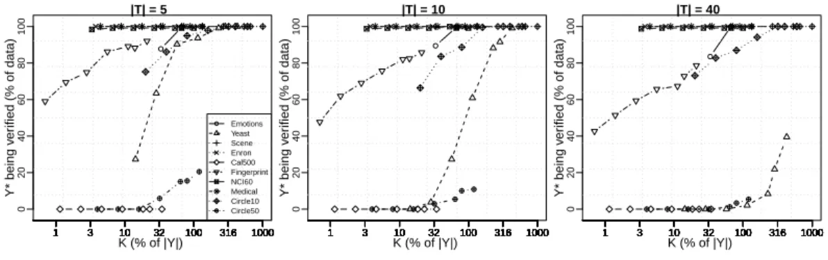
Figure 1: Percentage of examples with provably optimaly∗being in theK-best lists plotted as a function ofK, scaled with respect to the number of microlabels in the dataset.
favorable as the tree-based methods, as MMCRF quite consistently trails to RTA and MAM in both microlabel and 0/1 error, except forCircle50where it outperforms other models. Finally, we notice that SVM, as a single label classifier, is very competitive against most multilabel methods for microlabel accuracy.
Exactness of inference on the collection of trees. We now study the empirical behavior of the inference (see Section 4) on the collection of trees, which, if taken as a single general graph, would call for solving anN P-hard inference problem. We provide here empirical evidence that we can perform exact inference on most examples in most datasets in polynomial time.
We ran theK-best inference on eleven datasets where the RTA models were trained with different amounts of spanning trees|T |={5,10,40}and values forK={2,4,8,16,32,40,60}. For each pa-rameter combination and for each example, we recorded whether theK-best inference was provably exact on the collection (i.e., if Lemma 7 was satisfied). Figure 1 plots the percentage of examples where the inference was indeed provably exact. The values are shown as a function ofK, expressed as the percentage of the number of microlabels in each dataset. Hence,100%meansK=`, which denotes low polynomial (Θ(n`2)) time inference in the exponential size multilabel space.
We observe, from Figure 1, on some datasets (e.g.,Medical,NCI60), that the inference task is very easy since exact inference can be computed for most of the examples even withK values that are below50% of the number of microlabels. By settingK = ` (i.e.,100%) we can perform exact inference for about90%of the examples on nine datasets with five trees, and eight datasets with
40trees. On two of the datasets (Cal500, Circle50), inference is not (in general) exact with low values ofK. AllowingKto grow superlinearly on`would possibly permit exact inference on these datasets. However, this is left for future studies.
Finally, we note that the difficulty of performing provably exact inference slightly increases when more spanning trees are used. We have observed that, in most cases, the optimal multilabely∗ is still on theK-best lists but the conditions of Lemma 7 are no longer satisfied, hence forbidding us to prove exactness of the inference. Thus, working to establish alternative proofs of exactness is a worthy future research direction.
6
Conclusion
The main theoretical result of the paper is the demonstration that if a large margin structured output predictor exists, then combining a small sample of random trees will, with high probability, generate a predictor with good generalization. The key attraction of this approach is the tractability of the inference problem for the ensemble of trees, both indicated by our theoretical analysis and supported by our empirical results. However, as a by-product, we have a significant added benefit: we do not need to know the output structure a priori as this is generated implicitly in the learned weights for the trees. This is used to significant advantage in our experiments that automatically leverage correlations between the multiple target outputs to give a substantive increase in accuracy. It also suggests that the approach has enormous potential for applications where the structure of the output is not known but is expected to play an important role.
References
[1] Ben Taskar, Carlos Guestrin, and Daphne Koller. Max-margin markov networks. In S. Thrun, L.K. Saul, and B. Sch¨olkopf, editors,Advances in Neural Information Processing Systems 16, pages 25–32. MIT Press, 2004.
[2] Martin J. Wainwright, Tommy S. Jaakkola, and Alan S. Willsky. MAP estimation via agree-ment on trees: message-passing and linear programming. IEEE Transactions on Information Theory, 51(11):3697–3717, 2005.
[3] Michael I. Jordan and Martin J Wainwright. Semidefinite relaxations for approximate inference on graphs with cycles. In S. Thrun, L.K. Saul, and B. Sch¨olkopf, editors,Advances in Neural Information Processing Systems 16, pages 369–376. MIT Press, 2004.
[4] Amir Globerson and Tommi S. Jaakkola. Approximate inference using planar graph decom-position. In B. Sch¨olkopf, J.C. Platt, and T. Hoffman, editors,Advances in Neural Information Processing Systems 19, pages 473–480. MIT Press, 2007.
[5] Hongyu Su and Juho Rousu. Multilabel classification through random graph ensembles. Ma-chine Learning, dx.doi.org/10.1007/s10994-014-5465-9, 2014.
[6] Robert G. Cowell, A. Philip Dawid, Steffen L. Lauritzen, and David J. Spiegelhalter. Proba-bilistic Networks and Expert Systems. Springer, New York, 1999.
[7] Thomas G¨artner and Shankar Vembu. On structured output training: hard cases and an efficient alternative. Machine Learning, 79:227–242, 2009.
[8] John Shawe-Taylor and Nello Cristianini. Kernel Methods for Pattern Analysis. Cambridge University Press, 2004.
[9] J. Rousu, C. Saunders, S. Szedmak, and J. Shawe-Taylor. Efficient algorithms for max-margin structured classification. Predicting Structured Data, pages 105–129, 2007.
[10] Kristin P. Bennett. Combining support vector and mathematical programming methods for classifications. In B. Sch¨olkopf, C. J. C. Burges, and A. J. Smola, editors,Advances in Kernel Methods—Support Vector Learning, pages 307–326. MIT Press, Cambridge, MA, 1999. [11] Nello Cristianini and John Shawe-Taylor. An Introduction to Support Vector Machines and
Other Kernel-Based Learning Methods. Cambridge University Press, Cambridge, U.K., 2000. [12] Andreas Argyriou, Theodoros Evgeniou, and Massimiliano Pontil. Convex multi-task feature
learning.Machine Learning, 73(3):243–272, 2008.
[13] Yevgeny Seldin, Franc¸ois Laviolette, Nicol`o Cesa-Bianchi, John Shawe-Taylor, and Peter Auer. PAC-Bayesian inequalities for martingales. IEEE Transactions on Information Theory, 58:7086–7093, 2012.
[14] Andreas Maurer. A note on the PAC Bayesian theorem.CoRR, cs.LG/0411099, 2004. [15] David McAllester. PAC-Bayesian stochastic model selection. Machine Learning, 51:5–21,
2003.
[16] Juho Rousu, Craig Saunders, Sandor Szedmak, and John Shawe-Taylor. Kernel-based learn-ing of hierarchical multilabel classification models. Journal of Machine Learning Research, 7:1601–1626, December 2006.