NBER WORKING PAPER SERIES
OPTIMAL SIMPLE AND IMPLEMENTABLE MONETARY AND FISCAL RULES
Stephanie Schmitt-Grohe Martin Uribe Working Paper10253
http://www.nber.org/papers/w10253
NATIONAL BUREAU OF ECONOMIC RESEARCH 1050 Massachusetts Avenue
Cambridge, MA 02138 January 2004
We thank for comments Tommaso Monacelli and seminar participants at University Bocconi, the Bank of Italy, and the CEPR-INSEAD Workshop on Monetary Policy Effectiveness. The views expressed herein are those of the authors and not necessarily those of the National Bureau of Economic Research.
©2004 by Stephanie Schmitt-Grohe and Martin Uribe. All rights reserved. Short sections of text, not to exceed two paragraphs, may be quoted without explicit permission provided that full credit, including © notice, is given to the source.
Optimal Simple and Implementable Monetary and Fiscal Rules Stephanie Schmitt-Grohe and Martin Uribe
NBER Working Paper No. 10253 January 2004
JEL No. E52, E61, E63
ABSTRACT
The goal of this paper is to compute optimal monetary and fiscal policy rules in a real business cycle model augmented with sticky prices, a demand for money, taxation, and stochastic government consumption. We consider simple policy rules whereby the nominal interest rate is set as a function of output and inflation, and taxes are set as a function of total government liabilities. We require policy to be implementable in the sense that it guarantees uniqueness of equilibrium. We do away with a number of empirically unrealistic assumptions typically maintained in the related literature that are used to justify the computation of welfare using linear methods. Instead, we implement a second-order accurate solution to the model. Our main findings are: First, the size of the inflation coefficient in the interest-rate rule plays a minor role for welfare. It matters only insofar as it affects the determinacy of equilibrium. Second, optimal monetary policy features a muted response to output. More importantly, interest rate rules that feature a positive response of the nominal interest rate to output can lead to significant welfare losses. Third, the optimal fiscal policy is passive. However, the welfare losses associated with the adoption of an active fiscal stance are negligible. Stephanie Schmitt-Grohe Department of Economics Duke University P.O. Box 90097 Durham, NC 27708 and NBER [email protected] Martin Uribe Department of Economics Duke University Durham, NC 27708-0097 and NBER [email protected]
1
Introduction
Recently, there has been an outburst of papers studying optimal monetary policy in economies with nominal rigidities.1 Most of these studies are conducted in the context of highly stylized
theoretical and policy environments. For instance, in most of this body of work it is assumed that the government has access to a subsidy to factor inputs financed with lump-sum taxes aimed at dismantling the inefficiency introduced by imperfect competition in product and factor markets. This assumption is clearly empirically unrealistic. But more importantly it undermines a potentially significant role for monetary policy, namely, stabilization of costly aggregate fluctuations around a distorted steady-state equilibrium.
A second notable simplification is the absence of capital accumulation. All the way from the work of Keynes (1936) and Hicks (1939) to that of Kydland and Prescott (1982) macroeconomic theories have emphasized investment dynamics as an important channel for the transmission of aggregate disturbances. It is therefore natural to expect that investment spending should play a role in shaping optimal monetary policy. Indeed it has been shown, that for a given monetary regime the determinacy properties of a standard Neo-Keynesian model can change dramatically when the assumption of capital accumulation is added to the model (Dupor, 2001).
A third important dimension along which the existing studies abstracts from reality is the assumed fiscal regime. It is standard practice in this literature to completely ignore fiscal policy. Implicitly, these models assume that the fiscal budget is balanced at all times by means of lump-sum taxation. In other words, fiscal policy is always assumed to be non-distorting and passive in the sense of Leeper (1991). However, empirical studies, such as Favero and Monacelli (2003), show that characterizing postwar U.S. fiscal policy as passive
at all times is at odds with the facts. In addition, it is well known theoretically that,
given monetary policy, the determinacy properties of the rational expectations equilibrium crucially depend on the nature of fiscal policy (e.g., Leeper, 1991). It follows that the design of optimal monetary policy should depend upon the underlying fiscal regime in a nontrivial fashion.
Fourth, model-based analyses of optimal monetary policy is typically restricted to economies in which long-run inflation is nil or there is some form of wide-spread indexation. As a re-sult, in the standard environments studied in the literature nominal rigidities have no real consequences for economic activity and thus welfare in the long-run. It follows that the assumptions of zero long-run inflation or indexation should not be expected to be
inconse-1See Rotemberg and Woodford (1997, 1999), Clarida, Gal´ı, and Gertler (1999), Gal´ı and Monacelli (2002),
quential for the form that optimal monetary policy takes. Because from an empirical point of view, neither of these two assumptions is particularly compelling for economies like the United States, it is of interest to investigate the characteristics of optimal policy in their absence.
Last but not least, more often than not studies of optimal policy in models with nominal rigidities are conducted in cashless environments.2 This assumption introduces an
inflation-stabilization bias into optimal monetary policy. For the presence of a demand for money creates a motive to stabilize the nominal interest rate rather than inflation.
Taken together the simplifying assumptions discussed above imply that business cycles are centered around an efficient non-distorted equilibrium. The main reason why these rather unrealistic features have been so widely adopted is not that they are the most empirically obvious ones to make nor that researchers believe that they are inconsequential for the nature of optimal monetary policy. Rather, the motivation is purely technical. Namely, the stylized models considered in the literature make it possible for a first-order approximation to the equilibrium conditions to be sufficient to accurately approximate welfare up to second order
(Woodford 2003, chapter 6).3 Any plausible departure from the set of simplifying
assump-tions mentioned above, with the exception of the assumption of no investment dynamics, would require approximating the equilibrium conditions to second order.
Recent advances in computational economics have delivered algorithms that make it fea-sible and simple to compute higher-order approximations to the equilibrium conditions of a general class of large stochastic dynamic general equilibrium models.4 In this paper, we
employ these new tools to analyze a model that relaxes all of the questionable assumptions mentioned above. The central focus of this paper is to investigate whether the policy conclu-sions arrived at by the existing literature regarding the optimal conduct of monetary policy are robust with respect to more realistic specifications of the economic environment. That is, we study optimal policy in a world where there are no subsidies to undo the distortions cre-ated by imperfect competition, where there is capital accumulation, where the government may follow active fiscal policy and may not have access to lump-sum taxation, where
nom-2Exceptions are Khan, King, and Wolman (2003) and Schmitt-Groh´e and Uribe (2004).
3We note that an accurate first-order approximation to the utility function around the non-stochastic
steady state can be obtained using a linear approximation to the equilibrium conditions. But such an approximation is of little use. For the first-order approximation of the unconditional expectation of the welfare function around the stochastic steady state equals the welfare function evaluated at the non-stochastic steady state. Similarly, the first-order approximation of the conditional expectation of the welfare function, given that the initial state is equal to the non-stochastic steady state, is the welfare function evaluated at the stochastic steady state. It follows that if the initial state of the economy is the non-stochastic steady state, then up to first-order all policies that preserve the non-non-stochastic steady state yield the same level of welfare.
inal rigidities induce inefficiencies even in the long run, and where there is a nonnegligible demand for money.
Specifically, this paper characterizes monetary and fiscal policy rules that are optimal within a family of implementable, simple rules in a calibrated model of the business cycle. In the model economy, business cycles are driven by stochastic variations in the level of total factor productivity and government consumption. The implementability condition requires policies to deliver uniqueness of the rational expectations equilibrium. Simplicity requires restricting attention to rules whereby policy variables are set as a function of a small number of easily observable macroeconomic indicators. Specifically, we study interest-rate feedback rules that respond to measures of inflation and output. We study six different specifications of those rules: backward-looking rules (where the interest rate responds to past inflation and output), contemporaneous rules (where the interest rate responds to current inflation and output), and forward-looking rules (where the interest rate responds to expected future inflation and output). For each of these three types of rule, we consider the cases of interest-rate smoothing (i.e., the past value of the interest interest-rate enters as an additional argument into the rule) and no interest-rate smoothing. We analyze fiscal policy rules whereby the tax revenue is set as an increasing function of the level of public liabilities.
Our main findings are: First, the precise degree to which the central bank responds to inflation in setting the nominal interest rate (i.e., the size of the inflation coefficient in the interest-rate rule) plays a minor role for welfare provided that the monetary/fiscal regime renders the equilibrium unique. For instance, in all of the many environments we consider, deviating from the optimal policy rule by setting the inflation coefficient in the interest-rate rule anywhere above unity and below -2 yields virtually the same level of welfare as the optimal rule. At the same time values of the inflation coefficient between -2 and 1 are associated either with no equilibrium of indeterminacy of equilibrium. Thus, the fact that optimal policy features an active monetary stance serves mainly the purpose of ensuring the uniqueness of the rational expectations equilibrium. Second, optimal monetary policy features a muted response to output. More importantly, not responding to output is critical from a welfare point of view. In effect, our results show that interest rate rules that feature a positive response of the nominal interest rate to output can lead to significant welfare losses. Third, the optimal fiscal policy is passive. However, the welfare losses associated with the adoption of an active fiscal stance are negligible.
Kollmann (2003) also considers welfare maximizing fiscal and monetary rules in a sticky price model with capital accumulation. He also finds that optimal monetary features a strong anti-inflation stance. However, the focus of his paper differs from ours in a number of dimensions. First, Kollmann does not consider the size of the welfare losses that are
associated with non-optimal rules, which is at center stage in our work. Second, in his paper the interest rate feedback rule is not allowed to depend on a measure of aggregate activity and as a consequences the paper does not identify the importance of not responding to output. Third, Kollmann limits attention to a cashless economy with zero long run inflation.
The remainder of the paper is organized in six sections. Section 2 presents the model. Section 3 presents the calibration of the model and discusses computational issues. Section 4 computes optimal policy in a cashless economy. Section 5 analyzes optimal policy in a monetary economy. Section 6 introduces fiscal instruments as part of the optimal policy design problem. Section 7 concludes.
2
The Model
The starting point for our investigation into the welfare consequences of alternative policy rules is an economic environment featuring a blend of neoclassical and neo-Keynesian ele-ments. Specifically, the skeleton of the economy is a standard real-business-cycle model with capital accumulation and endogenous labor supply driven by technology and government spending shocks. Four sources of inefficiency separate our model from the standard RBC framework: (a) nominal rigidities in the form of sluggish price adjustment. A later section incorporates sticky wages as a second source of nominal rigidity. (b) A demand for money motivated by a working-capital constraint on labor costs. (c) time-varying distortionary taxation. And (d) monopolistic competition in product markets. These four elements of the model provide a rationale for the conduct of monetary and fiscal stabilization policy.
2.1
Households
The economy is populated by a continuum of identical households. Each household has preferences defined over consumption, ct, and labor effort, ht. Preferences are described by the utility function
E0
∞
X t=0
βtU(ct, ht), (1) where Et denotes the mathematical expectations operator conditional on information avail-able at time t, β ∈ (0,1) represents a subjective discount factor, and U is a period utility index assumed to be strictly increasing in its first argument, strictly decreasing in its second argument, and strictly concave. The consumption good is assumed to be a composite good
produced with a continuum of differentiated goods,cit,i∈[0,1], via the aggregator function ct = Z 1 0 cit1−1/ηdi 1/(1−1/η) , (2)
where the parameter η > 1 denotes the intratemporal elasticity of substitution across dif-ferent varieties of consumption goods. For any given level of consumption of the composite
good, purchases of each variety i in period t must solve the dual problem of minimizing
total expenditure, R01Pitcitdi, subject to the aggregation constraint (2), where Pit denotes the nominal price of a good of variety i at time t. The optimal level of cit is then given by
cit= Pit Pt −η ct, (3)
where Pt is a nominal price index given by
Pt ≡ Z 1 0 Pit1−ηdi 1 1−η . (4)
This price index has the property that the minimum cost of a bundle of intermediate goods yielding ct units of the composite good is given byPtct.
Households are assumed to have access to a complete set of nominal contingent claims. Their period-by-period budget constraint is given by
Etrt,t+1xt+1+ct+it +τtL=xt+ (1−τtD)[wtht +utkt] + ˜φt, (5)
where rt,s is a stochastic discount factor, defined so that Etrt,sxs is the nominal value in period t of a random nominal payment xs in periods ≥t. The variable kt denotes capital,
it denotes investment, ˜φt denotes profits received from the ownership of firms net of income taxes, τtD denotes the income tax rate, and τ
L
t denotes lump-sum taxes. The capital stock
is assumed to depreciate at the constant rate δ, so the evolution of capital is given by
kt+1 = (1−δ)kt+it. (6)
The investment good is assumed to be a composite good made with the aggregator func-tion (2). Thus, the demand for each intermediate good i ∈ [0,1] for investment purposes, denoted iit, is given by iit = (Pit/Pt)
−η
it. Households are also assumed to be subject to a borrowing limit that prevents them from engaging in Ponzi schemes. The household’s prob-lem consists in maximizing the utility function (1) subject to (5), (6), and the no-Ponzi-game
borrowing limit. The first-order conditions associated with the household’s problem are Uc(ct, ht) = λt, (7) λtrt,t+1 =βλt+1 Pt Pt+1 −Uh(ct, ht) Uc(ct, ht) =wt(1−τtD), (8) and λt =βEt λt+1 (1−τtD+1)ut+1+ 1−δ . (9)
It is apparent from these first-order conditions that the income tax distorts both the leisure-labor choice and the decision to accumulate capital over time.
Let Rt denote the gross one-period, risk-free, nominal interest in period t. Then by a no-arbitrage condition, Rt must equal the inverse of the period-t price of a portfolio that pays one dollar in every state of period t+ 1. That is,
Rt = 1
Etrt,t+1
.
Combining this expression with the optimality conditions associated with the household’s problem yields λt =βRtEtλt+1 Pt Pt+1 . (10)
2.2
The Government
The consolidated government prints money, Mt, issues one-period nominally risk-free bonds,
Bt, collects taxes in the amount ofPtτt, and faces an exogenous expenditure stream,gt. Its period-by-period budget constraint is given by
Mt+Bt =Rt−1Bt−1+Mt−1+Ptgt−Ptτt.w
The variable gt denotes per capita government spending on a composite good produced via
the aggregator (2). We assume, maybe unrealistically, that the government minimizes the cost of producing gt. Thus, we have that the public demand for each type i of intermediate goods, git, is given by git = (Pit/Pt)
−η
gt. Let `t−1 ≡ (Mt−1 +Rt−1Bt−1)/Pt−1 denote total
real government liabilities outstanding at the beginning of period t in units of period t−1 goods. Also, let mt ≡ Mt/Pt denote real money balances in circulation and πt ≡ Pt/Pt−1
written as
`t = (Rt/πt)`t−1+Rt(gt −τt)−mt(Rt−1) (11)
We wish to consider various alternative fiscal policy specifications that involve possibly both lump sum and distortionary income taxation. Total tax revenue, τt, consist of revenue
from lump-sum taxation, τL
t , and revenue from income taxation,τ D
t yt. That is,
τt =τtL+τ D
t yt. (12)
The fiscal regime is defined by the following rule
τt =γ0+γ1(`t−1−`) +γ2 gt + Rt−1−1 Rt−1 `t−1−mt−1 πt , (13)
whereγ0,γ1, γ2, and` are parameters. According to this rule, the fiscal authority sets total
tax receipts as a function of two variables, the deviation of total government liabilities `t−1
from a target level`and the level of the real secondary fiscal deficit,gt+ Rt−1−1 Rt−1 `t−1−mt−1 πt . We consider four different fiscal policy regimes. In the first two regimes all taxes are lump sum at all times, and in the latter two all taxes are distortionary at all times. For each case, lump-sum or distortionary taxation, we consider two different feedback rules. One feedback rule postulates that each period tax receipts are adjusted in response to variations in the secondary fiscal deficit in such a way that the secondary deficit is zero. We refer to this rule as a balanced-budget rule. Under the second policy total tax collection is set as a linear function of the deviation of the stock of government liabilities from their target value. We refer to this policy as liability targeting. The parameterizations associated with the four cases then are:
(i) lump-sum taxes and balanced-budget rule: τtD =γ0 =γ1 = 0 andγ2 = 1
(ii) lump-sum taxes and liability targeting: τD
t = 0, γ2 = 0;
(iii) income taxation and balanced-budget rule: τL
t =γ0 =γ1 = 0 andγ2 = 1;
(iv) income taxation and liability targeting: τL
t = 0 and γ2 = 0.
The a fiscal policy consisting of lump-sum taxation and a balanced-budget rule a is Ricardian policy in the sense that fiscal variables play no role for price level determination.5 The fiscal
policy featuring lump-sum taxes and liability targeting is motivated by the one considered in Leeper (1991). As Leeper shows depending on the size of the coefficient γ1, this fiscal
5As shown in Schmitt-Groh´e and Uribe (2000), this claim is correct only if the nominal interest rate is
expected to be strictly positive in the long-run, which is an assumption we will maintain throughout the paper.
policy regime is active or passive. In particular for γ1 greater than but close to the real
rate of interest, fiscal policy will be passive, or Ricardian. We consider liability targeting because it allows for the possibility that fiscal policy is active, or in the terminology of Leeper (1991) active. In that case fiscal considerations will play an important role for price level determination. This feature distinguishes our analysis from most of the existing related literature where it is assumed from the outset (either explicitly or implicitly) that fiscal policy is passive. It then follows that optimal monetary policy must be active by construction because otherwise a determinate equilibrium usually does not exist. Our analysis is thus broader because it allows for the possibility that a combination of active fiscal and passive monetary policy is optimal.
We assume that the monetary authority sets the short-term nominal interest rate accord-ing to a simple feedback rule belongaccord-ing to the followaccord-ing class of Taylor (1993)-type rules
ln(Rt/R∗) =αRln(Rt−1/R∗) +απEtln(πt−i/π∗) +αyEtln(yt−i/y); i=−1,0,1, (14)
where Rt denotes the gross one-period nominal interest rate, yt denotes output in period t,
y denotes the non-stochastic steady-state level of output, and R∗, π∗, αR, απ,, and αy are parameters. The index i can take three values 1, 0, and -1. In the case thati = 1, we refer to the interest rate rule as backward looking, when i= 0 we call the rule contemporaneous, and wheni=−1 the rule is said to be forward looking. The reason why we focus on interest rate feedback rules belonging to this class is that they are easily implementable. For all of its arguments are generally available macroeconomic indicators.
We note that the type of monetary policy rules that are typically analyzed in the related literature require no less information on the part of the policymaker than the feedback rule given in equation (14). This is because the rules most commonly studied feature an output gap measure defined as deviations of output from the level that would obtain in the absence of nominal rigidities. Computing the flexible-price level of aggregate activity requires the policymaker to know not just the deterministic steady state of the economy, but also the joint distribution of all the shocks driving the economy and the current realizations of such shocks.
2.3
Firms
Each good’s variety i∈[0,1] is produced by a single firm in a monopolistically competitive environment. Each firm i produces output using as factor inputs capital services, kit, and
labor services, hit. The production technology is given by
ztF(kit, hit),
where the function F is assumed to be homogenous of degree one, concave, and strictly
increasing in both arguments. The variable zt denotes an exogenous and stochastic produc-tivity shock.
It follows from our analysis of private and public absorption behavior that the aggregate demand for good i, ait ≡cit+iit+git is given by
ait= (Pit/Pt)−ηat,
where at ≡ct+it+gt denotes aggregate absorption.
We introduce money in the model by assuming that wage payments are subject to a cash-in-advance constraint of the form
mit≥νwthit, (15) where mit denotes the demand for real money balances by firm i in period t and ν ≥ 0 is a parameter denoting the fraction of the wage bill that must be backed with monetary assets.
Real profits of firm i at date t expressed in terms of the composite good are given by6
φit≡
Pit
Pt
ait−utkit−wthit−(1−R−t 1)mit. (16)
Implicit in this specification of profits is the assumption that firms rent capital services from a centralized market, which requires that this factor of production can be readily reallocated across industries. This is a common assumption in the related literature (e.g., Christiano et al., 2003; Kollmann, 2003; Carlstrom and Fuerst, 2003; and Rotemberg and Woodford, 1992). A polar assumption is that capital is sector specific, as in Woodford (2003) and Sveen and Weinke (2003). Both assumptions are clearly extreme. A more realistic treatment of investment dynamics would incorporate a mix of firm-specific and homogeneous capital.
We assume that the firm must satisfy demand at the posted price. Formally, we impose
ztF(kit, hit)≥ Pit Pt −η at. (17)
The objective of the firm is to choose contingent plans for Pit, hit, kit and mit so as to
maximize the present discounted value of profits, given by Et ∞ X s=t rt,sPsφis.
Throughout our analysis, we will focus on equilibria featuring a strictly positive nominal interest rate. This implies that the cash-in-advance constraint (15) will always be binding. Then, letting mcitbe the Lagrange multiplier associated with constraint (17), the first-order conditions of the firm’s maximization problem with respect to capital and labor services are, respectively, mcitztFh(kit, hit) =wt 1 +νRt −1 Rt and mcitztFk(kit, hit) =ut.
Notice that because all firms face the same factor prices and because they all have access to the same homogenous-of-degree-one production technology, the capital-labor ratio,kit/hit and marginal cost, mcit, are identical across firms.
Prices are assumed to be sticky `a la Calvo (1983) and Yun (1996). Specifically, each
period a fraction α ∈ [0,1) of randomly picked firms is not allowed to change the nominal price of the good it produces. The remaining (1−α) firms choose prices optimally. Suppose firm igets to choose the price in period t, and let ˜Pit denote the chosen price. This is set so as to maximize the expected present discounted value of profits. That is, ˜Pit maximizes
Et ∞ X s=t rt,sPsαs−t P˜it Ps !1−η as−uskis−wshis[1 +ν(1−Rs−1)] +mcis " zsF(kis, his)− ˜ Pit Ps !−η as #) .
The associated first-order condition with respect to ˜Pit is
Et ∞ X s=t rt,sαs−t ˜ Pit Ps !−1−η as " mcis− η−1 η ˜ Pit Ps # = 0. (18)
According to this expression, firms whose price is free to adjust in the current period, pick a price level such that some weighted average of current and future expected differences between marginal costs and marginal revenue equals zero.
2.4
Equilibrium and Aggregation
We limit attention to a symmetric equilibrium in which all firms that get to change their
price in each period indeed choose the same price. We thus drop the subscript i. So the
firm’s demands for capital and labor aggregate to
mctztFh(kt, ht) =wt 1 +νRt−1 Rt (19) and mctztFk(kt, ht) = ut. (20)
Similarly, the sum of all firm-level cash-in-advance constraints holding with equality yields the following aggregate relationship between real balances and the wage bill:
mt =νwtht. (21)
From (4), it follows that the aggregate price index can be written as
Pt1−η =αP
1−η
t−1 + (1−α) ˜P 1−η t
Dividing this expression through by Pt1−η, one obtains
1 =απt−1+η + (1−α)˜p
1−η
t , (22)
where ˜pt denotes the relative price of any good whose price was adjusted in periodtin terms of the composite good.
At this point, most of the related literature using the Calvo-Yun apparatus, proceeds to linearize equations (18) and (22) around a deterministic steady state featuring zero infla-tion. This strategy yields the famous simple (linear) neo-Keynesian Phillips curve involving inflation and marginal costs (or the output gap). In the present study one cannot follow this strategy for two reasons. First, we do not wish to restrict attention to the case of zero long-run inflation. For we believe it is unrealistic, as it is contradicted by the post-war economic history of most industrialized countries. Second, we refrain from making the set of highly special assumptions that allow welfare to be approximated accurately from a first-order approximation to the equilibrium conditions. One of these assumptions is the ex-istence of factor-input subsidies financed by lump-sum taxes aimed at ensuring the perfectly competitive level of long-run employment. Another assumption that makes it appropriate to use first-order approximations to the equilibrium conditions for welfare evaluation is that
of a cashless economy. In the model under study we introduce a demand for money and calibrate its size to US postwar experience.
Our approach makes it necessary to retain the non-linear nature of the equilibrium con-ditions and in particular of equation (18). It is convenient to rewrite this expression in a recursive fashion that does away with the use of infinite sums. To this end, we define two new variables, x1 t and x 2 t. Let x1t ≡ Et ∞ X s=t rt,sαs−t ˜ Pt Ps !−1−η asmcs = P˜t Pt !−1−η atmct +Et ∞ X s=t+1 rt,sαs−t ˜ Pt Ps !−1−η asmcs = P˜t Pt !−1−η atmct +αEtrt,t+1 ˜ Pt ˜ Pt+1 Et+1 ∞ X s=t+1 rt+1,sαs−t−1 ˜ Pt+1 Ps !−1−η asmcs = P˜t Pt !−1−η atmct +αEtrt,t+1 ˜ Pt ˜ Pt+1 !−1−η x1t+1 = p˜−t 1−ηatmct +αβEt λt+1 λt πtη+1 ˜ pt ˜ pt+1 −1−η x1t+1. (23) Similarly, let x2t ≡ Et ∞ X s=t rt,sαs−t ˜ Pt Ps !−1−η as ˜ Pt Ps = p˜−t ηat +αβEt λt+1 λt πtη+1−1 ˜ pt ˜ pt+1 −η x2t+1, (24)
Using the two auxiliary variables x1t and x
2
t, the equilibrium condition (18) can be written as: η η−1x 1 t =x 2 t. (25)
Naturally, the set of equilibrium conditions includes a resource constraint. Such a re-striction is typically of the typeztF(kt, ht) =ct+it+gt. In the present model, however, this restriction is not valid. This is because the model implies relative price dispersion across varieties. This price dispersion, which is induced by the assumed nature of price stickiness, is inefficient and entails output loss. To see this, start with equilibrium condition (17) stating
that supply must equal demand at the firm level: ztF(kit, hit) = (ct+it+gt) Pit Pt −η .
Integrating over all firms and taking into account that the capital-labor ratio is common across firms, we obtain
htztF kt ht ,1 = (ct+it +gt) Z 1 0 Pit Pt −η di, where ht ≡ R1 0 hitdi and kt ≡ R1
0 kitdi denote the aggregate per capita levels of labor and
capital services in period t. Let st ≡ R1 0 Pit Pt −η
di. Then we have
st = Z 1 0 Pit Pt −η di = (1−α) ˜ Pt Pt !−η + (1−α)α ˜ Pt−1 Pt !−η + (1−α)α2 ˜ Pt−2 Pt !−η +. . . = (1−α) ∞ X j=0 αj P˜t−j Pt !−η = (1−α)˜p−t η+απ η tst−1
Summarizing, the resource constraint in the present model is given by the following two expressions yt = zt st F(kt, ht) (26) yt =ct+it+gt (27) st = (1−α)˜p −η t +απ η tst−1, (28)
withs−1 given. The state variablestsummarizes the resource costs induced by the inefficient price dispersion present in the Calvo-Yun model in equilibrium.
Three observations are in order about the dispersion measure st. First, st is bounded below by 1. That is, price dispersion is always a costly distortion in this model. Second, in an economy where the non-stochastic level of inflation is nil, i.e., when π = 1, up to first order the variable st is deterministic and follows a univariate autoregressive process of the form ˆst =αsˆt−1. Thus, the underlying price dispersion, summarized by the variable st, has
no real consequences up to first order in the stationary distribution of endogenous variables. This means that studies that restrict attention to linear approximations to the equilibrium
conditions around a noninflationary steady-state are justified to ignore the variable st. But this variable must be taken into account if one is interested in higher-order approximations to the equilibrium conditions or if one focuses on economies without long-run price stability (π∗ 6= 1). Omitting s
t in higher-order expansions would amount to leaving out certain
higher-order terms while including others. Finally, when prices are fully flexible, α = 0, we have that ˜pt = 1 and thus st = 1. (Obviously, in a flexible-price equilibrium there is no price dispersion across varieties.).7
A stationary competitive equilibrium is a set of processes ct, ht, λt, wt, τtD, ut, mct,
kt+1, Rt, it, yt, st, ˜pt, πt, τt, τtL, `t, mt, x1t, and x
2
t for t = 0,1, . . . that remain bounded in some neighborhood around the deterministic steady-state and satisfy equations (6)-(14), (19)-(28) and either τtL = 0 (in the absence of lump-sum taxation) orτ
D
t = 0 (in the absence of distortionary taxation), given initial values fork0, s−1, and`−1, and exogenous stochastic
processes gt and zt.
3
Computation, Calibration, and Welfare Measure
We wish to find the monetary and fiscal policy rule combination that is optimal and im-plementable within the simple family defined by equations (13) and (14). For a policy to be implementable, we require that it ensure local uniqueness of the rational expectations equilibrium. In turn, for an implementable policy to be optimal, the contingent plans for consumption and hours of work associated with that policy must yield the highest level of lifetime utility, within the particular class of policy rules considered, given the current state of the economy. Formally, we look for implementable policies that maximize
Vt ≡Et
∞
X j=0
βjU(ct+j, ht+j),
given that at time t all state variables take their steady-state values. That is to say, these policies are optimal conditional on the current state being the steady state.
3.1
Computation
Given the complexity of the economic environment we study in this paper, we are forced to characterize an approximation to lifetime utility. Up to first-order accuracy, Vt is equal to
7Here we add a further note on aggregation. The variable ˜φ
t introduced in the household’s budget constraint (5) is related to aggregate profits,φt ≡
R1 0 φitdiby the relation ˜φt= (1−τ D t )φt−τtD(1−R −1 t )mt. This relationship states that working-capital expenditures are not tax deductible. We introduce this twist in the tax code so that the base for distortionary taxation is simply value added, or aggregate demand,yt.
its non-stochastic steady-state value. Because all the monetary and fiscal policy regimes we consider imply identical non-stochastic steady states, to a first-order approximation all of those policies yield the same level of welfare. To determine the higher-order welfare effects of alternative policies one must therefore approximate Vt to a higher order than one. For an expansion ofVt to be accurate up to second order, it is in general required that the solution to the equilibrium conditions—the policy functions—also be accurate up to second order. In particular, approximations to the policy functions based on a first-order expansion of the equilibrium conditions would result in general in an incorrect second-order approximation of the welfare criterionVt. In this paper, we compute second-order accurate solutions to policy
functions using the methodology and computer code of Schmitt-Groh´e and Uribe (2004).
In characterizing optimal policy we search over the coefficients αR, απ, and αy of the monetary policy rule (14) and, when we consider fiscal policies other than balanced-budget rules, over the coefficient γ1 of the fiscal policy rule (13).
3.2
Calibration
We compute a second-order approximation to the policy functions around the non-stochastic steady state of the model. The coefficients of the approximated policy functions are them-selves functions of the deep structural parameters of the model. Therefore, one must assign numerical values to these structural parameters.
The time unit is meant to be a quarter. We calibrate the model to the U.S. economy. We assume that the period utility function is given by
U(c, h) = [c(1−h)
γ]1−σ −1
1−σ . (29)
We set σ = 2, so that the intertemporal elasticity of consumption, holding constant hours
worked, is 0.5. In the business-cycle literature, authors have used values of 1/σ as low as 1/3 (e.g., Rotemberg and Woodford, 1992) and as high as 1 (e.g., King, Plosser, and Rebelo, 1988). Our choice of σ falls in the middle of this range.
The production function is assumed to be of the Cobb-Douglas type
F(k, h) =kθh1−θ,
where θ describes the cost share of capital. We set θ equal to 0.3, which is consistent with the empirical regularity that in the U.S. economy wages represent about 70 percent of total cost.
an annual real rate of interest of 4 percent (Prescott, 1986). We set η, the price elasticity of demand, so that in steady state the value added markup of prices over marginal cost is 28 percent (see Basu and Fernald, 1997). We require the share of government purchases in value added to be 17 percent in steady state, which is in line with the observed U.S. postwar average. The steady-state inflation rate is assumed to be 4.2 percent per year. This value is consistent with the average U.S. GDP deflator growth rate over the period 1960-1998. The annual depreciation rate is taken to be 10 percent, a value typically used in business-cycle studies.
Based on the observations that two thirds of M1 are held by firms (Mulligan, 1997) and that annual GDP velocity is 0.17 in U.S. data (for a 1960 to 1999 sample), we calibrate the ratio of working capital to quarterly GDP to 0.45(= 0.17×2/3×4). This parameterization implies that ν = 0.82, which means that firm’s must pay 82 percent of their wage bill with cash.
We set the ratio of tax revenues to GDP to 0.2, which is consistent with the 1997-2001 average of the US federal budget receipts to GDP ratio.8
Following Sbordone (2002) and Gal´ı and Gertler (1999), we assign a value to α, the
fraction of firms that cannot change their price in any given quarter, that implies that on
average firms change prices every 3 quarters. We set the preference parameter γ so that
in the simple economy without money and lump-sum taxes, agents allocate on average 20 percent of their time to work, as is the case in the U.S. economy according to Prescott (1986). Given the other calibrated parameters and the steady-state conditions, the implied value of
γ is 3.4080. The associated Frisch elasticity of labor supply then is about 1.5, which lies well within the range of values typically used in the real business cycle literature.
We equate the parameters R∗, π∗, and y appearing in the monetary policy rule (14) to
the steady-state values of R, π, andy, respectively.
Government purchases are assumed to follow a univariate autoregressive process of the form
ˆ
gt =ρggˆt−1+
g t,
where ˆgt ≡ [lngt −lnG] denotes the percentage deviation of government purchases from steady state and G denotes the steady-state level of government purchases. The first-order autocorrelation, ρg, is set to 0.9 and the standard deviation of
g
t to 0.0074. The second
source of uncertainty in the model are productivity shocks. They are also assumed to follow
8Together with the assumed value for the share of government purchases in value added, the value assigned
to the tax-to-GDP ratio implies a long-run debt-to-GDP ratio of about 90 percent. This value is high relative to the US out-of-war experience, but closer to what is observed in other G7 countries. A lower steady-state debt-to-GDP ratio could be accommodated by allowing for government transfers.
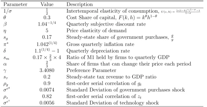
Table 1: Calibrated Parameters
Parameter Value Description
1/σ 12 Intertemporal elasticity of consumption, U(c, h) =[c(1−h)γ]1
−σ−1 1−σ
θ 0.3 Cost Share of capital, F(k, h) =kθh1−θ
β 1.04−1/4 Quarterly subjective discount rate
η 5 Price elasticity of demand
sg 0.17 Steady-state share of government purchases, gy
π∗ 1.042(1/4) Gross quarterly inflation rate
δ 1.1(1/4)−1 Quarterly depreciation rate
sm 0.17× 23 ×4 Ratio of M1 held by firms to quarterly GDP
α 23 Share of firms that can change their price each period
γ 3.4080 Preference Parameter
sτ 0.2 Steady-state tax revenue to GDP ratio
ρg 0.9 first-order serial correlation of gt
σg 0.0074 Standard Deviation of government purchases shock
ρz 0.82 first-order serial correlation of zt
σz 0.0056 Standard Deviation of technology shock
a univariate autoregressive process
lnzt =ρzlnzt−1+zt,
whereρz = 0.82 and the standard deviation ofzt is 0.0056. Table 1 summarizes the calibra-tion of the model.
3.3
The Welfare Measure
We measure the level of utility associated with a particular monetary and fiscal policy spec-ification as follows. Let the contingent plans for consumption and hours associated with a particular monetary and fiscal regime be denoted bycrt and h
r
t. Then we measure welfare as the conditional expectation of lifetime utility as of time zero, that is,
welfare =V0 ≡E0
∞
X t=0
βtU(crt, hrt).
In addition, we assume that at time zero all state variables of the economy equal their respective steady-state values. Note that we are departing from the usual practice of iden-tifying the welfare measure with the unconditional expectation of lifetime utility. Because different policy regimes will in general be associated with a different stochastic steady state, using unconditional expectations of welfare amounts to not taking into account the
transi-tional dynamics leading to the stochastic steady state. Because the non-stochastic steady state is the same across all policy regimes we consider, our choice of computing expected welfare conditional on the initial state being the nonstochastic steady state ensures that the economy begins from the same initial point under all possible polices. Therefore, our strategy will deliver the constrained optimal monetary/fiscal rule associated with a particu-lar initial state of the economy. It is of interest to investigate the robustness of our results with respect to alternative initial conditions. For, in principle, the welfare ranking of the alternative polices will depend upon the assumed value for (or distribution of) the initial state vector.9
We compute the welfare cost of a particular monetary and fiscal regime relative to the optimized rule as follows. Consider two policy regimes, a reference policy regime denoted by r and an alternative policy regime denoted by a. Then we define the welfare associated with policy regime r as
V0r =E0 ∞ X t=0 βtU(crt, h r t), wherecr t andh r
t denote the contingent plans for consumption and hours under policy regime
r. Similarly, define the welfare associated with policy regime a as
V0a=E0 ∞ X t=0 βtU(cat, h a t).
Let λ denote the welfare cost of adopting policy regime a instead of the reference policy
regimer. We measureλ as the fraction of regime r’s consumption process that a household would be willing to give up to be as well off under regime a as under regime r. Formally, λ
is implicitly defined by V0a =E0 ∞ X t=0 βtU((1−λ)crt, hrt).
For the particular functional form for the period utility function given in equation (29), the above expression can be written as
V0a = E0 ∞ X t=0 βtU((1−λ)crt, hrt) = (1−λ)1−σV0r+ (1−λ)1−σ−1 (1−σ)(1−β).
Solving for λ we obtain the following expression for the welfare cost associated with policy
regime a vis-´a-vis the reference policy regime r in percentage terms welfare cost =λ×100 = " 1− (1−σ)Va 0 + (1−β) −1 (1−σ)V0r+ (1−β)−1 1/(1−σ)# ×100. (30)
4
A Cashless Economy
We first consider a non-monetary economy by setting
ν = 0
in equation (15). The fiscal authority is assumed to have access to lump-sum taxes and to follow a balanced-budget rule. That is, the fiscal policy rule is given by equations (12) and (13) with
γ0 =γ1 =τtD = 0,
and
γ2 = 1.
This case is of interest for it most resembles the case studied in the related literature on optimal policy (see Clarida, Gal´ı, and Gertler, 1999, Woodford, 2003, chapter 4, and the references cited therein). This body of work studies optimal monetary policy in the context of a cashless economy with nominal rigidities and no fiscal authority. For analytical purposes, the absence of a fiscal authority is equivalent to modeling a government that operates under a perpetual balanced-budget rule and collects all of its revenue via lump-sum taxation. We wish to highlight, however, two important differences between the economy
studied here and the one typically considered in the related literature. Namely, in our
economy there is capital accumulation and there do not exist subsidies to factor inputs that undo the distortions arising from monopolistic competition. The latter difference is of consequence for the solution method that can be applied to the optimal policy problem. As shown by Woodford (2003, chapter 6), one can use a first-order approximation to the policy function to obtain an accurate second-order approximation to the utility function under certain assumptions. One of the necessary assumptions is that the government has access to factor input subsidies to undo the monopolistic distortion. Without this ad-hoc subsidy scheme, first-order approximations to the policy functions no longer deliver a second-order accurate approximation to the utility function. Thus, in this case one must approximate the policy functions up to second order to obtain a second-order accurate approximation to the level of welfare, which is what we do in this paper.
The top panel of table 2 presents the coefficients of some optimized policy rules and of some other monetary policy specifications. For this economy, we consider five different monetary policies. Two of those are constrained optimal rules. In one case, we search over the monetary feedback rule coefficients απ and αy while restricting αR to be zero. This case is labeled no smoothing in the table. For each parameter we search over a grid from -3 to 3 with a step of 0.1, that is, we consider 61 values for each parameter. For a policy rule to be optimal, we require that (a) the associated equilibrium be locally unique; (b) the equilibrium is locally unique everywhere in a neighborhood of radius 0.15 around the optimized coefficients; and (c) welfare attains a local optimum within that neighborhood. Condition (a) rules out parameter specifications that render the equilibrium indeterminate. Requirement (b) eliminates parameter configurations that are in the vicinity of a bifurcation point. The reason for excluding such points is that welfare computations near a bifurcation point may be inaccurate. Condition (c) rules out selecting an element of a sequence of policy parameters associated with increasing welfare that converges to a bifurcation point. We find that the best no-smoothing rule requires that the monetary authority not respond to output and choose an inflation coefficient of 3. Note that this is the largest value of απ that we allow in our search. Our conjecture is that if we left this parameter unconstrained, then optimal policy would call for an arbitrarily large inflation coefficient.10 The reason is that in that case under the optimal policy inflation would in effect be forever constant so that the economy would be characterized by zero inflation volatility.
One might wonder why the representative household prefers to live in a world with con-stant positive inflation rather than in one with varying inflation. This question is motivated by the fact that the non-stochastic steady-state level of inflation in our model is positive, which means that the distortions introduced by price stickiness are present even in the steady state. Some intuition for why constant inflation is optimal when the long-run level is constrained exogenously to be positive can be gained from the fact that in our model the non-stochastic steady-state level of welfare is globally concave in the steady-state infla-tion rate with a maximum at zero inflainfla-tion. Thus, loosely speaking households dislike to randomize around the constant level of long-run inflation.
We next study a case in which the central bank can smooth interest rates over time, formally, we allow the coefficient αR on the lagged interest rate to take any value between -3 and 3. Our grid search yields that the optimal policy coefficients are απ = 3, αy = 0, and
αR= 0.9. These coefficients imply that the long-run coefficient on inflation is 30, the largest value it can take given our grid size. So, again, as in the case without smoothing optimal
10We experimented enlarging theα
π range up to [−7,7]. We found that the optimal rule always picks the highest value allowed for the inflation coefficient.
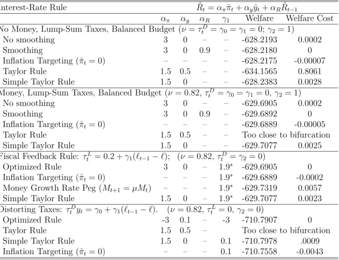
Table 2: Optimal Interest-Rate Rules in the Sticky-Price Model
Interest-Rate Rule Rˆt =απˆπt +αyyˆt+αRRˆt−1
απ αy αR γ1 Welfare Welfare Cost
No Money, Lump-Sum Taxes, Balanced Budget (ν =τD
t =γ0 =γ1 = 0; γ2 = 1)
No smoothing 3 0 – – -628.2193 0.0002
Smoothing 3 0 0.9 – -628.2180 0
Inflation Targeting (ˆπt = 0) – – – – -628.2175 -0.00007
Taylor Rule 1.5 0.5 – – -634.1565 0.8061
Simple Taylor Rule 1.5 0 – – -628.2383 0.0028
Money, Lump-Sum Taxes, Balanced Budget (ν = 0.82,τtD =γ0 =γ1 = 0, γ2 = 1)
No smoothing 3 0 – – -629.6905 0.0002
Smoothing 3 0 0.9 – -629.6892 0
Inflation Targeting (ˆπt = 0) – – – – -629.6889 -0.00005
Taylor Rule 1.5 0.5 – – Too close to bifurcation
Simple Taylor Rule 1.5 0 – – -629.7077 0.0025
Fiscal Feedback Rule: τL
t = 0.2 +γ1(`t−1 −`); (ν = 0.82,τtD =γ2 = 0)
Optimized Rule 3 0 – 1.9∗ -629.6905 0
Inflation Targeting (ˆπt = 0) – – – 1.9∗ -629.6889 -0.0002
Money Growth Rate Peg (Mt+1 =µMt) – – – 1.9∗ -629.7319 0.0057
Simple Taylor Rule 1.5 0 – 1.9∗ -629.7077 0.0023
Distorting Taxes: τD
t yt =γ0+γ1(`t−1−`). (ν = 0.82, τtL = 0, γ2 = 0)
Optimized Rule -3 0.1 – -3 -710.7907 0
Taylor Rule 1.5 0.5 – Too close to bifurcation
Simple Taylor Rule 1.5 0 – 0.1 -710.7978 .0009
Inflation Targeting (ˆπt = 0) – – – 0.1 -710.7558 -0.0043
Notes: (1) Rt denotes the gross nominal interest rate, πt denotes the gross in-flation rate, and yt denotes output. (2) For any variable xt, its non-stochastic steady-state value is denoted byx, and its log-deviation from steady state by ˆxt ≡ ln(xt/x). (3) In all cases, the parametersαπ,αy, andαRare restricted to lie in the interval [−3,3]. (4) Welfare is defined as follows: Let V(gt, zt, Rt−1, `t−1, st−1, kt)
denote the equilibrium level of lifetime utility of the representative household in period t given that period’s state (gt, zt, Rt−1, `t−1, st−1, kt). Then welfare is
defined as V(g, z, R, `, s, k). (5) The welfare cost is measured relative to opti-mized rule and is defined as the percentage decrease in the consumption process associated with the optimal rule necessary to make the level of welfare under the optimized rule identical to that under the considered policy. Thus, a positive figure indicates that welfare is higher under the optimized rule than under the alternative policy.
∗In the economy with a fiscal feedback rule for lump-sum taxes, any passive fiscal
Figure 1: Determinacy Regions and Welfare in the Cashless Economy −3 −2 −1 0 1 2 3 −3 −2 −1 0 1 2 3 απ α R (α y=0)
Note: A dot represents a parameter combination for which the equilibrium is determinate. A circle denotes that the welfare cost of the policy relative to the optimal policy (i.e. απ = 3, αy = 0, and αR= 0.9) is less than 0.05 percent.
policy calls for a large response to inflation deviations in order to stabilize the inflation rate and for no response to deviation of output from the steady state. The level of welfare associated with this policy is -628.2180. This is slightly higher than -628.2193, the level of welfare associated with the optimal policy without smoothing. But the difference is not very large. As shown in column 7 of table 2, agents would be willing to give up just 0.0002, that is, 2 one-thousands, of one percent of their consumption stream under the optimized rule with smoothing to be as well off as under the optimized policy without smoothing. For all practical purposes we regard this difference in the level of welfare as negligible.
This finding let us to investigate by how much welfare indeed changes as we vary the coefficients of the policy rule. Figure 1 shows that given that the central bank does not
respond to output, αy = 0, varying απ and αR between the -3 and 3 typically leads to welfare losses of less than five one-hundredth of one percent. The graph shows with a dot the combinations ofαπ andαRthat render the rational expectations equilibrium determinate and with a circle the combinations for which the welfare costs are less than 0.05 percent. The figure makes two important points. First, it shows that there are quite a large number of απ and αR combinations for which the equilibrium fails to be locally unique (the blank area in the figure). This is for example the case for positive values of απ and αR such that the policy stance is passive in the long run, that is, for απ and αR combinations such that 0< απ/(1−αR)<1. This finding is consistent with those obtained in economic environments that abstract from capital accumulation. It is thus reassuring that this particular abstraction appears to be of no consequence for the finding that long-run passive policy is inconsistent with local uniqueness of the rational expectations equilibrium. Similarly, with rules in which the response to inflation and past interest rates is positive we find that determinacy obtains for policies that are active in the long run (απ/(1−αR)>1). Second, and more importantly, the graph shows that basically all parameterization of the monetary feedback rule that deliver determinacy yield welfare differences in the order of at most five one-hundredth of one percent of the consumption stream associated with the optimized rule. This implies a simple policy prescription, namely, that any parameter combination that implies that the policy stance is acyclical and active in the long run is equally desirable from a welfare point of view.
One possible reaction to the finding that determinacy-preserving variations in απ and
αR have little welfare consequences may be that in the class of model we consider welfare is always very flat in a rather large neighborhood around the optimum, so that it does not really matter what the government does. However, this is not the case in our economy. Recall that in the welfare calculations underlying figure 1 the response coefficient on output,
αy, was kept constant at zero. Indeed, interest-rate policy rules that lean against the wind by raising the nominal interest rate when output is above trend can be associated with large welfare costs.
4.1
The importance of not responding to output
Figure 2 illustrates the consequences of introducing a cyclical component to the interest-rate rule. It shows that the welfare costs of varying αy can be large, thereby underlining the importance of not responding to output. The solid line shows the welfare cost of deviating from the optimal output coefficient (αy = 0) while keeping the remaining two coefficients of the interest-rate rule at their optimal values (απ = 3 and αR = 0.9). For positive values of
Figure 2: The Importance of Not Responding to Output: The Cashless Economy −1.5 −1 −0.5 0 0.5 1 1.5 2 2.5 3 −0.1 0 0.1 0.2 0.3 0.4 0.5 0.6 0.7 0.8 0.9 αy, απ, or α R welfare cost (%) αy απ αR
Note: The welfare cost is relative to the optimized policy rule, i.e., απ = 3,
the welfare cost is one-tenth of one percent of the consumption stream associated with the optimized rule. For negative output response coefficients, the welfare cost also rapidly rises. For an αy of -0.5 the welfare cost is two tenth of one percent. For values below -0.5, the equilibrium ceases to be locally unique and thus the solid line ends.
To highlight the importance of not responding to output, figure 2 also shows the welfare consequences of varying either απ, shown with a circled line, or αR, shown with the dashed line. Again, as the value of one parameter varies, the values assigned to the remaining two parameters are held constant at their optimal levels. For both the inflation coefficient απ and the inertial coefficient αR, the welfare costs of deviating from the optimal values are negligible. Thus these findings suggest that bad policy can have huge welfare costs in our model and that big policy mistakes are committed when policy makers are unable to resist the temptation to respond to output fluctuations. It follows that sound monetary policy calls for sticking to the basics of responding to inflation alone.11
A question that emerges naturally from our forgoing results is why cyclical monetary policy is so disruptive. An intuition often offered for why a policy of leaning against the wind is not appropriate in response to supply shocks such as a technology shock, is that under leaning against the wind the nominal interest rate rises whenever output rises. This increase in the nominal interest rate in turn hinders prices falling by as much as marginal costs causing markups to increase. With an increase in markups, output does not increase as much as it would have otherwise, preventing the efficient rise in output (see, for example, Rotemberg and Woodford, 1997). This explanation requires that in response to a positive supply shock, the central bank raises the nominal interest by more or lowers it by less in the case that αy is positive as compared to the case in which αy is nil. But this is not what happens in the class of sticky-price models to which ours belongs.
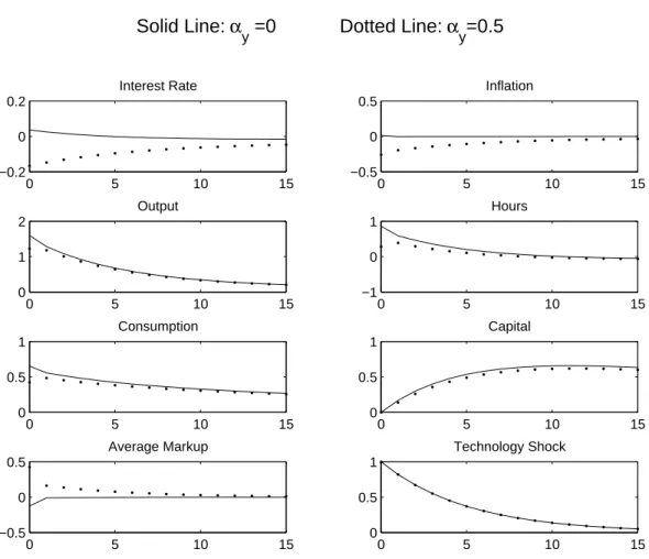
Figure 3 depicts the impulse of a number of endogenous variables of interest to a one-percent increase in the exogenous productivity factorzt. The figure displays impulse response functions associated with two alternative values for the output coefficient in the interest-rate rule, the one called for by the optimized rule (αy = 0) and a positive one (αy = 0.5). In response to the positive productivity shock, the nominal interest rate increases in the case of an acyclical monetary stance, but falls when the central bank leans against the wind. This implication of the model may appear as surprising at first. For one would be inclined to expect that introduction of a procyclical component into the interest rate rule would induce a stronger positive response of the nominal interest rate to a positive supply shock. But further inspection of the structure of the model reveals that the intuition is indeed more
11A number of other authors have argued that countercyclical interest rate policy may be undesirable (e.g.,
Figure 3: Impulse Response to a 1 percent technology shock 0 5 10 15 −0.2 0 0.2 Interest Rate 0 5 10 15 −0.5 0 0.5 Inflation 0 5 10 15 0 1 2 Output 0 5 10 15 −1 0 1 Hours 0 5 10 15 0 0.5 1 Consumption 0 5 10 15 0 0.5 1 Capital 0 5 10 15 −0.5 0 0.5 Average Markup Solid Line: α y =0 Dotted Line: αy=0.5 0 5 10 15 0 0.5 1 Technology Shock
Note: The feedback rule coefficients areαπ = 3, αy = 0 or 0.5, and αR= 0.9. For all variables with the exception of the inflation rate and the nominal interest rate, the impulse responses are shown in percent deviations from the steady state. For inflation and the nominal interest rate, deviations from steady state in percentage points, rather than percent deviations, are shown.
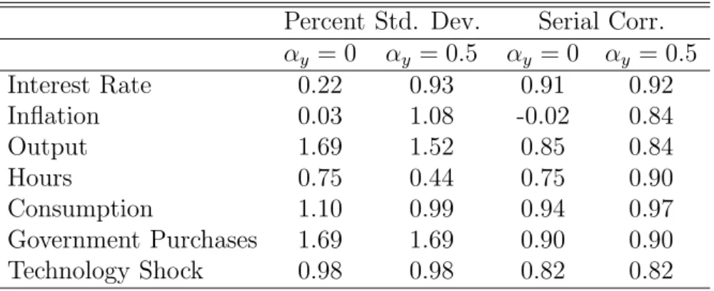
Table 3: Standard Deviations and Serial Correlations
Percent Std. Dev. Serial Corr.
αy = 0 αy = 0.5 αy = 0 αy = 0.5 Interest Rate 0.22 0.93 0.91 0.92 Inflation 0.03 1.08 -0.02 0.84 Output 1.69 1.52 0.85 0.84 Hours 0.75 0.44 0.75 0.90 Consumption 1.10 0.99 0.94 0.97 Government Purchases 1.69 1.69 0.90 0.90 Technology Shock 0.98 0.98 0.82 0.82
Note. The standard deviations of inflation and the nominal interest rate are expressed in percentage points per year.
subtle. The dynamics of inflation in this model are driven primarily by the Fisher effect (i.e., the interest rate is the sum of expected future inflation and the real interest rate) and the interest rate rule, linking the interest rate to current inflation and output. A simple flexible price example will suffice to gather intuition for the equilibrium dynamics of inflation. Consider an endowment economy where output follows a univariate autoregressive process of the formEtyˆt+1 =ρyˆt withρ∈(0,1). All variables are expressed in log-deviations from their respective deterministic-steady-state values. In equilibrium, the Euler equation that prices riskless nominal bonds (or Fisher equation) is of the form −σyˆt = ˆRt −Etπˆt+1 −σEtyˆt+1,
where σ measures the elasticity of intertemporal substitution. The interest-rate rule is of the form ˆRt = αππˆt + αyyˆt, with απ > 1. The non-explosive solution to this system of stochastic linear difference equations is ˆπt =Dπyˆt where Dπ ≡[σ(1−ρ) +αy]/(ρ−απ)<0 and ˆRt =DRˆyt, where DR = [απσ(1−ρ) +αyρ]/(ρ−απ)<0. Note that as output becomes highly persistent (ρ → 1), we have that both Dπ and DR converge to αy/(1−απ). In this case we have that a positive output innovation produces a negative response of inflation and the interest rate when the Fed has a countercyclical stance (αy >0), but has no effect on the equilibrium level of these variables when monetary policy is acyclical (αy = 0). Moreover, the decline in inflation and interest rates are larger the greater is the output coefficient of the interest-rate feedback rule.
The argument in the previous paragraph suggests that cyclical monetary policy results in higher inflation volatility. Table 3 confirms this conjecture. It shows that in our sticky-price model the standard deviation of inflation falls from 108 basis points per annum to 3 basis points as αy decreases from 0.5 to zero. In the context of nominal rigidities, inflation volatility entails a welfare cost because it generates inefficient price dispersion.
4.2
Inflation Targeting
Our forgoing suggest that a policy of complete inflation stabilization may be the optimal
policy prescription in our economy. Thus, we were led to compute the level of welfare
associated with inflation targeting. Under inflation targeting the central bank is assumed to do something that results in a constant inflation rate over the business cycle. We do not discuss how such a policy may actually be implemented. The level of welfare for this regime is -628.2175, which is higher than the level of welfare associated with the optimized rule with smoothing. But the welfare benefit is only 0.00007, which means that one would have to raise the consumption stream under the optimized rule by 0.00007 percent to make agents as happy as they are under an inflation targeting regime.
Finally, we show the welfare costs associated with a Taylor rule featuring an inflation coefficient of 1.5 and an output coefficient of either 0.5 or of 0. In the former case, the welfare costs are large ( 0.8 percent) as expected from the analysis presented in figure 2 whereas in the latter case the welfare costs are negligible as was already implicit in figure 1.
4.3
Backward- and Forward-Looking Interest-Rate Rules
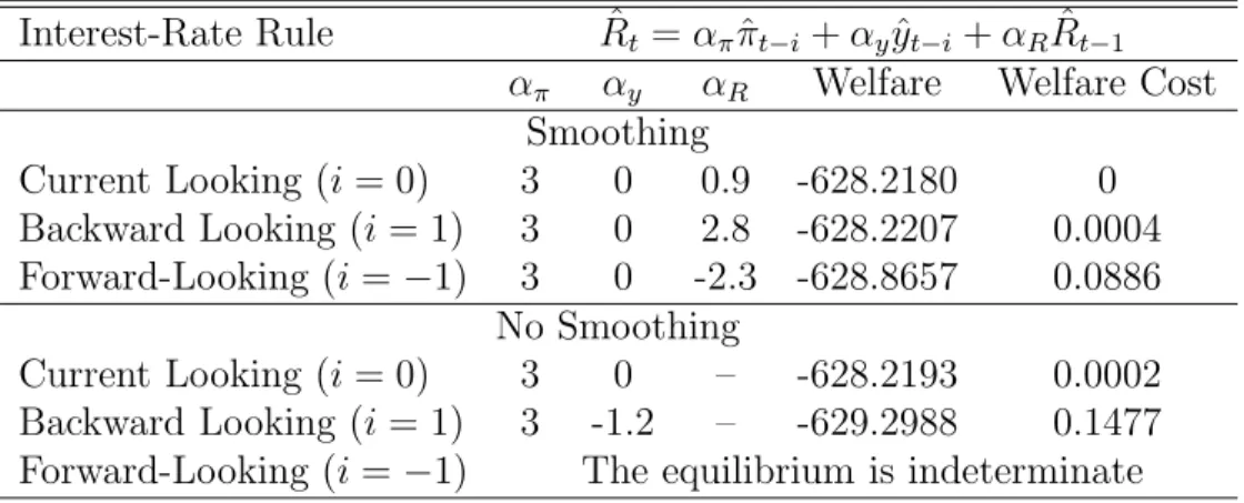
An important issue in monetary policy is what measures of inflation and aggregate activity the central bank should respond to. In particular, a question that has received considerable attention among academic economists and policymakers is whether the monetary authority should target past, current, or expected future values. Here we address this question by com-puting optimal backward- and forward-looking interest-rate rules. That is, in equation (14) we let i take the values −1 and +1. Table 4 presents the results. To facilitate comparison, the table reproduces the optimal rule coefficients for the case in which the central bank re-sponds to measures of current inflation and output (i= 0) from table 2. The top panel of the table shows that there are no welfare gains from targeting expected future values of inflation and output as opposed to current or lagged values of these macroeconomic indicators. The best specification is one where the monetary authority responds to current values of the two target variables. Not responding to output continues to be optimal under backward- and forward-looking rules.
In the absence of smoothing (αR= 0) both backward- and forward-looking interest-rate rules appear to be disruptive. In the case of a forward-looking rule, the rational expectations equilibrium is indeterminate for all values of the inflation and output coefficients in the inter-val [-3,3]. This result is in line with those obtained by Carlstrom and Fuerst (2003). These authors consider an environment similar to ours and characterize determinacy of equilibrium for interest-rate rules that depend only on the rate of inflation. Our indeterminacy result
Table 4: Optimal Backward- and Forward-Looking Interest-Rate Rules Interest-Rate Rule Rˆt =αππˆt−i+αyyˆt−i+αRRˆt−1
απ αy αR Welfare Welfare Cost
Smoothing Current Looking (i= 0) 3 0 0.9 -628.2180 0 Backward Looking (i= 1) 3 0 2.8 -628.2207 0.0004 Forward-Looking (i=−1) 3 0 -2.3 -628.8657 0.0886 No Smoothing Current Looking (i= 0) 3 0 – -628.2193 0.0002 Backward Looking (i= 1) 3 -1.2 – -629.2988 0.1477
Forward-Looking (i=−1) The equilibrium is indeterminate
Notes: See notes to table 2.
for forward-looking rules thus extends the findings of Carlstrom and Fuerst to the case in which output enters into the feedback rule.12
5
A Monetary Economy
We next introduce money into the model by assuming that the parameter ν denoting the
fraction of the wage bill that must be cash financed takes the value shown on table 1. All other aspects of the model, including the fiscal policy specification, are as in the cashless economy analyzed in the previous section. Unlike in the cashless economy, in this model complete inflation stabilization may not continue to be optimal because it is associated with fluctuations in the nominal interest rate, which in turn now distort the effective wage rate via the working-capital constraint. So, there will be a trade off between inflation stabilization to neutralize the distortions stemming from sluggish price adjustment and nominal interest rate stabilization to dampen the distortions introduced by the working capital constraint.
This tradeoff, however, does not seem to be quantitatively important. In effect, when we search over the coefficients of the interest rate feedback rule, απ, αy, and αR, we recover the same optimal coefficient values as in the economy without money, that is, απ takes the largest value included in our grid, 3, the output coefficient is zero, αy = 0, and the central bank makes intensive use of interest rate smoothing, αR = 0.9. The level of welfare under the optimal rule is -629.6892.13 If we do not allow for interest rate smoothing, that is, if we
12Carlstrom and Fuerst (2003) comment that including output in the interest rate rule would have minor
effects on the local determinacy conditions (see their footnote 4).
constrain αR to be zero, it is still optimal not to respond to output,αy = 0 and to make the inflation response of the interest rate as large as possible (απ = 3). Utility falls slightly to -629.6905. The welfare cost of eliminating smoothing is just 0.0002 percent of consumption, which is again economically negligible.
As in the cashless case, we find that the precise magnitude of the inflation coefficient and the smoothing coefficient play no rule, provided that they imply a locally unique rational
expectations equilibrium and αy is held at zero. This point is clearly communicated by
figure 4. As before, a dot in the figure indicates that this particular (suboptimal) combination ofαπ andαR results in a determinate equilibrium and a circle indicates that the welfare cost associated with it is less than 0.05 percent of the optimal consumption stream. Variations in the output response coefficient of the interest rate feedback rule,αy continue to be associated with large welfare losses particularly ifαy is large. Figure 5 plots with a solid line the welfare losses as a function of αy. Equilibrium is locally unique only for values of αy between -0.3 and 2.4, given απ = 3 and αR = 0.9. The welfare costs exceed 0.05 percent for αy greater than 0.6. Consider αy = 0.6. Then, given αR = 0.9 the long-run coefficient on output is 6 and the welfare loss is only 0.0424 percent. On the other hand, for αy = 2, for example, the welfare cost is 1.15 percent of consumption, which is a relatively large number. By contrast, variations in αR and αy over the range [−3,3] lead to welfare costs of at most 0.0013 and 0.0004 percent, respectively.
A further similarity between the cashless and the cash-in-advance economies is that infla-tion targeting dominates all other policies considered. In sum, in this economy, the tradeoff between inflation stabilization and interest rate stabilization introduced by nominal rigidities on the one hand and the monetary exchange friction on the other hand, is overwhelmingly resolved in favor of inflation stabilization.
5.1
Difference Rules
In motivating the interest-rate rules considered above, we argue that they demand little sophistication on the part of policymakers because the variables involved in the rules are few and easily observable. However, one might argue that because the variables included in the rules we have been working with are expressed in deviations from the non-stochastic steady state, implementation requires knowledge of the deterministic steady state by the central bank. The non-stochastic steady state is, however, non-observable. Thus, the assumed rule the economy without money. Given our assumption that the nominal interest rate is positive in the non-stochastic steady state welfare must be lower in the economy with money than in the one without money. Both in the cashless economy and in the model with money, welfare under the optimized rule is higher than in the non-stochastic steady state. The reason must be that the presence of monopolistic competition induces higher output and consumption on average in a stochastic economy than in a non-stochastic one.
Figure 4: Determinacy Regions and Welfare in the Monetary Economy −3 −2 −1 0 1 2 3 −3 −2 −1 0 1 2 3 απ α R (α y=0)
Figure 5: The Importance of Not Responding to Output: The Monetary Economy −1.5 −1 −0.5 0 0.5 1 1.5 2 2.5 3 0 0.5 1 1.5 2 2.5 3 αy, απ, or α R welfare cost (%) αy απ αR