The Costs of Fiscal Inflexibility

ISSN 1749-8279

Working Paper Series

WEF 0005

The Costs of Fiscal Inflexibility

Campbell Leith

University of Glasgow

Simon Wren-Lewis

University of Exeter

March 2006

The Costs of Fiscal In

fl

exibility

Campbell Leith

University of Glasgow

Simon Wren-Lewis

University of Exeter

Abstract: Extending Gali and Monacelli (2004), we build an N-country open economy model, where each economy is subject to sticky wages and prices and, potentially, has access to sales and income taxes as well as government spending asfiscal instruments. We examine an economy either as a small open economy operating underflexible exchange rates or as a member of a monetary union. In a small open economy when all threefiscal instruments are freely available, we show analytically that the welfare impact of technology and mark-up shocks can be completely eliminated (in the sense that policy can replicate the efficientflex price equilibrium), whether policy acts with discretion or commitment. How-ever, once any one of thesefiscal instruments is excluded as a stabilisation tool, costs can emerge. Using simulations, wefind that the usefulfiscal instrument in this case (in the sense of reducing the welfare costs of the shock) is either income taxes or sales taxes. In constrast, having government spending as an instrument contributes very little.

The results for an individual member of a monetary union facing an idiosyn-cratic technology shock (where monetary policy in the union does not respond) are very different. First, even with all fiscal instruments freely available, the technology shock will incur welfare costs. Government spending is potentially useful as a stabilisation device, because it can act as a partial substitute for monetary policy. Finally, sales taxes are more effective than income taxes at reducing the costs of a technology shock under monetary union. If all three taxes are available, they can reduce the impact of the technology shock on the union member by around a half, compared to the case wherefiscal policy is not used.

Finally we consider the robustness of these results to two extensions. Firstly, introducing government debt, such that policy makers take account of the debt consequences of usingfiscal instruments as stabilisation devices, and, secondly, introducing implementation lags in the use offiscal instruments. We find that the need for debt sustainability has a very limited impact on the use of fiscal instruments for stabilisation purposes, while implementation lags can reduce, but not eliminate, the gains fromfiscal stabilisation.

∗_{We would like to thank Andrew Hughes-Hallett, Tatiana Kirsanova, Patrick}

Minford, Charles Nolan, Alan Sutherland, David Vines, Mike Wickens and par-ticipants at seminars at HM Treasury, St Andrews University and the MMF for very helpful discussions in the process of drafting this paper. All errors remain our own. We are also grateful to the ESRC, Grant No.RES-156-25-003, forfi -nancial assistance. Address for correspondence: Campbell Leith, Department of Economics, University of Glasgow, Adam Smith Building, Glasgow G12 8RT. E-mail c.b.leith@socsci.gla.ac.uk.

1

Overview

There has been a wealth of recent work deriving optimal monetary policy for both closed and open economies utilising New Classical Keynesian Synthesis models where the structural model and the description of policy makers’ objec-tives are consistently microfounded. (See for example, Woodford (2003) for a comprehensive treatment of the closed economy case, and Claridaet al (2001) for its extension to the open economy case.) More recently, some papers have extended this analysis to include various forms of activefiscal policy, although only a few in the context of open economies or a monetary union.1 Even when

fiscal policy has been analysed, however, the number of activefiscal instruments considered has tended to be small (generally one, occasionally two). This omis-sion is important since different fiscal instruments have quite different effects, and their efficacy varies across shocks and policy regimes, as we show below. Additionally, when fiscal instruments are introduced they are typically assumed to be asflexible as interest rates, which may give a misleading indication of their effectiveness.This omission is important since different fiscal instruments have quite different effects, and their efficacy varies across shocks and policy regimes. Additionally, whenfiscal instruments are introduced they are typically assumed to be asflexible as interest rates.

The focus on monetary policy rather than a combination of monetary and

fiscal policy probably reflects three factors. Thefirst is that, when the only nom-inal inertia in the economy involves price setting, optimal monetary policy can completely offset the impact of technology or preference shocks (by reproducing the flex price equilibrium) if exchange rates are flexible. However, this is no longer the case if there is also inertia in nominal wage setting, and we allow for both forms of nominal inertia in this paper. As we shall show, this introduces an important potential role for using tax as a stabilisation instrument. Sec-ond, there is much lessflexibility in movingfiscal policy instruments, although this inflexibility varies between countries (and instruments), and may not be immutable. In this paper we explicitly examine the costs of this inflexibility, either by introducing implementation lags, or by ruling out the use of particular instruments completely. A third concern may be that usingfiscal instruments for stabilisation may compromise the control of public sector debt. Although

this may involve political economy concerns which are outside the scope of this paper, we do generalise our model to include public sector debt.

We consider open economies in which there are three potentialfiscal instru-ments alongside monetary policy: government spending, income taxes and sales taxes. As well as the small open economy case, we also consider the case of an individual member of a monetary union, using a framework set out in Gali and Monacelli (2004) (henceforth GM). We examine optimal policies when all

fiscal instruments are available and fullyflexible (under commitment or discre-tion), and then look at the impact on welfare if there are lags in using these instruments, or if only a subset of instruments are available for short term sta-bilisation.

Our benchmark regime is for a small open economy, when all three fiscal instruments are freely available. Here we can show analytically that thefi rst-best solution can be achieved. However, once any one of thesefiscal instruments is excluded as a stabilisation tool, significant costs emerge. Using simulations, wefind that the usefulfiscal instrument in this case (in the sense of reducing the welfare costs of a technology shock) is either income taxes or sales taxes. In constrast, having government spending as an instrument contributes very little. This is also true of mark-up shocks, where only a tax instrument which can directly offset the inflationary pressures created by the shock is effective in dealing with the shock.

The results for an individual member of a monetary union facing an idiosyn-cratic technology shock (where monetary policy in the union has no reason to respond) are very different. First, even with all fiscal instruments freely avail-able, the technology shock will imply that variables deviate from their efficient levels, implying welfare costs. Government spending is potentially useful as a stabilisation device, because it can act as a partial substitute for monetary policy. Finally, sales taxes are more effective than income taxes at reducing the costs of a technology shock under monetary union. For both a small open economy and a monetary union member, wefind that implementation/reaction lags significantly reduce, but do not eliminate, the welfare benefits of fiscal stabilisation.

Initially, our analysis assumes the existence of a lump sum tax whose sole purpose is to balance the budget each period. As Ricardian Equivalence holds, changes in this tax have no impact on the economy, but allow us to ignore the government’s budget constraint in our analysis. In an extension to our model, we consider the case where lump-sum taxes are not available to offset the consequences for the government’s budget constraint of usingfiscal instruments as stabilisation devices. Allowing for the impact of changes in policy on debt has only a small impact on our results. This is because it is optimal either to accomodate the impact offiscal shocks on debt (i.e. debt has a random walk character, as in Benigno and Woodford (2005)), or that the optimal speed for correcting debt disequilibrium is slow (see Leith and Wren-Lewis (2005a)).

Our next section derives the model. Section 3 outlines the social planner’s problem such that we can write our model in ‘gap’ form. This representation of the model can also be used to derive a quadratic approximation to welfare. In

section 4 we derive the optimal pre-commitment policies for the open economy and for a continuum of economies participating in monetary union. Section 5 simulates such economies to quantify the relative contribution of alternative

fiscal instruments to macroeconomic stability. In this section we also consider the importance of implementation lags in relation to fiscal variables. Section 6 adds government debt to the model and assesses the importance of the con-straints imposed by the need forfiscal solvency. A conclusion summarises the main results.

2

The Model

This section outlines our model. We focus on the economic problems facing economic agents in a single ‘home’ economy, but it should be noted this economy exists in a world economy containing an infinite number of economies which are symmetrical to this one. We shall consider optimal policy when such economies operate underflexible exchange rates or when they form a monetary union. As noted above, our model is similar in structure to GM, but we allow for the existence of sticky wages as well as prices and introduce distortionary sales and income taxes. The model is further extended by introducing government debt in section 6.

2.1

Households

There are a continuum of households of size one, who differ in that they pro-vide differentiated labour services tofirms in their economy. However, we shall assume full asset markets, such that, through risk sharing, they will face the same budget constraint and make the same consumption plans even if they face different wage rates due to stickiness in wage-setting. As a result the typical household will seek to maximise the following objective function,

E0

∞

X

t=0

βtU(Ct, N(k)t, Gt) (1)

where C,G and N are a consumption aggregate, a public goods aggregate, and labour supply respectively. Here the only notation referring to the specific household,k, indexes the labour input, as fullfinancial markets will imply that all other variables are constant across households.

The consumption aggregate is defined as

C= C

1−α

H CFα

(1₋α)(1−α)_αα (2)

where, if we drop the time subscript, all variables are commensurate. CH is a

composite of domestically produced goods given by

CH = ( Z 1 0 CH(j) ε−1 ² dj) ² ²−1 (3)

where j denotes the good’s type or variety. The aggregateCF is an aggregate across countriesi CF = ( Z 1 0 C η−1 η i di) η η−1 (4)

whereCi is an aggregate similiar to (3). Finally the public goods aggregate is

given by G= ( Z 1 0 G(j)ε−²1dj) ² ²−1 (5)

which implies that public goods are all domestically produced. The elasticity of substitution between varieties² >1is common across countries. The parameter

αis (inversely) related to the degree of home bias in preferences, and is a natural measure of openness.

The budget constraint at timet is given by

Z 1 0 PH,t(j)CH,t(j)dj+ Z 1 0 Z 1 0

Pi,t(j)Ci,t(j)djdi+Et{Qt,t+1Dt+1}(6)

= Πt+Dt+WtN(k)t(1−τt)−Tt

where Pi,t(j) is the price of variety j imported from country i expressed in

home currency,Dt+1 is the nominal payoffof the portfolio held at the end of

periodt,Πis the representative household’s share of profits in the imperfectly competitivefirms,W are wages,τ is an wage income tax rate, andT are lump sum taxes. Qt,t+1 is the stochastic discount factor for one period ahead payoffs.

Households must first decide how to allocate a given level of expenditure across the various goods that are available. They do so by adjusting the share of a particular good in their consumption bundle to exploit any relative price dif-ferences - this minimises the costs of consumption. Optimisation of expenditure for any individual good implies the demand functions given below,

CH(j) = ( PH(j) PH )−²CH (7) Ci(j) = ( Pi(j) Pi )−²Ci (8)

where we have price indices given by

PH = ( Z 1 0 PH(j)1−²dj) 1 1−² (9) Pi = ( Z 1 0 Pi(j)1−²dj) 1 1−² (10) It follows that Z 1 0 PH(j)CH(j)dj = PHCH (11) Z 1 0 Pi(j)Ci(j)dj = PiCi (12)

Optimisation across imported goods by country implies Ci= ( Pi PF )−ηCF (13) where PF = ( Z 1 0 P_i1−ηdi)1−1η (14) This implies Z 1 0 PiCidi=PFCF (15)

Optimisation between imported and domestically produced goods implies

PHCH = (1−α)P C (16)

PFCF = αP C (17)

where

P =P_H1−αP_Fα (18)

is the consumer price index (CPI). The budget constraint can therefore be rewritten as

PtCt+Et{Qt,t+1Dt+1}=Πt+Dt+WtN(k)t(1−τt)−Tt (19)

2.1.1 Households’ Intertemporal Consumption Problem

Thefirst of the household’s intertemporal problems involves allocating consump-tion expenditure across time. For tractability assume (following GM) that (1) takes the specific form

E0 ∞ X t=0 βt(lnCt+χlnGt− (N(k)t)1+ϕ 1 +ϕ ) (20)

In addition, assume that the elasticity of substitution between the baskets of foreign goods produced in different countries is η = 1 (this is equivalent to adopting logarithmic utility in the aggregation of such baskets).

We can then maximise utility subject to the budget constraint (19) to obtain the optimal allocation of consumption across time,

β( Ct Ct+1

)( Pt Pt+1

) =Qt,t+1 (21)

Taking conditional expectations on both sides and rearranging gives

βRtEt{( Ct Ct+1 )( Pt Pt+1 )_}= 1 (22)

whereRt= _Et{Q1_t,t+1} is the gross return on a riskless one period bond paying

offa unit of domestic currency int+ 1. This is the familiar consumption Euler equation which implies that consumers are attempting to smooth consumption over time such that the marginal utility of consumption is equal across periods (after allowing for tilting due to interest rates differing from the households’ rate of time preference).

A log-linearised version of (22) can be written as

ct=Et{ct+1}−(rt−Et{πt+1}−ρ) (23)

where lowercase denotes logs (with an important exception forgnoted below),

ρ= _β1 ₋1, andπt=pt−pt−1is consumer price inflation.

2.1.2 Households’ Wage-Setting Behaviour

We now need to consider the wage-setting behaviour of households. We assume that firms need to employ a CES aggregate of the labour of all households in the domestic production of consumer goods. This is provided by an ‘aggregator’ that aggregates the labour services of all households in the economy as,

N= ∙Z 1 0 N(k)²−²w1_dk ¸ ²w ²w−1 (24) where N(k) is the labour provided by household k to the aggregator. We allow the degree of labour differentiation to vary in response to iid shocks which introduce the possibility of wage mark-up shocks. Accordingly the demand curve facing each household is given by,

N(k) =

µ_W(k)

W

¶−²w

N (25)

where N is the CES aggregate of labour services in the economy which also equals the total labour services employed byfirms,

N =

Z 1 0

N(j)dj (26)

whereN(j)is the labour employed byfirmj. The price of this labour is given by the wage index,

W = ∙Z 1 0 W(k)1−²w_dk ¸1−²w (27) The household’s objective function for the setting of its nominal wage is given by, Et Ã_∞ X s=0 (θwβ)s ∙ Λt+s W(k)t Pt+s (1₋τt+s)N(k)t+s− (N(k)t+s)1+ϕ 1 +ϕ ¸! (28)

whereΛt+s=Ct−+1sis the marginal utility of real post-tax income andN(k) =

³

W(k)

W

´−²w

N is the demand curve for the household’s labour. The first order condition from this problem can be combined with the aggregate wage index (see Leith and Wren-Lewis (2005b)), to give a log-linearised expression for wage-inflation dynamics,

πw_t =βEtπw_t+1+ λw (1 +ϕ²w)

(ϕnt−wt+ct+pt−ln(1−τt) + ln(µwt)) (29)

whereλw = (1−θwβ_θ)(1_w −θw) and µwt is the wage-markup in the absence of wage

stickiness2_{. Note that the forcing variable in this New Keynesian Phillips curve}

(NKPC) is a log-linearsed measure of the extent to which wages are not at the level implied by the labour supply decision that would hold underflexible wages.

2.2

Price and Exchange Rate Identities

The bilateral terms of trade are the price of country i’s goods relative to home goods prices,

Si=

Pi

PH

(30) The effective terms of trade are given by

S = PF PH (31) = exp Z 1 0 (pi−pH)di (32)

Recall the definition of consumer prices,

P =P_H1−αP_Fα (33)

Using the definition of the effective terms of trade this can be rewritten as,

P =PHSα (34)

or in logs as

p=pH+αs (35)

where s=pF −pH is the logged terms of trade. By taking first-differences it

follows that,

πt=πH,t+α(st−st−1) (36)

There is assumed to be free-trade in goods, such that the law of one price holds for individual goods at all times. This implies,

Pi(j) =εiPii(j) (37)

2_{A time subscript has been added to what would otherwise be the steady-state wage} mark-up to reflect that fact that we shall subject this variable to iid mark-up shocks below.

whereεiis the bilateral nominal exchange rate andP_ii(j)is the price of county i’s good j expressed in terms of country i’s currency. Aggregating across goods this implies, Pi=εiPii (38) wherePi i = ³R1 0 Pii(j)1−²dj ´ 1 1−² . From the definition of PF we have,

PF = ( Z 1 0 P_i1−ηdi)1−1η (39) = ( Z 1 0 ¡ εiPii ¢1−η di)1−1η (40) In log-linearised form, pF = Z 1 0 (ei+pii)di (41) = e+p∗ (42)

where e = R₀1eidi is the log of the nominal effective exchange rate, pii is the

logged domestic price index for country i, and p∗ ₌ R1

0 piidi is the log of the

world price index. For the world as a whole there is no distinction between consumer prices and the domestic (world) price level.

Combining the definition of the terms of trade and the result just obtained gives

s = pF−pH (43)

= e+p∗₋pH (44)

Now consider the link between the terms of trade and the real exchange rate. (Note that although we have free trade and the law of one price holds for individual goods, our economies do not exhibit PPP since there is a home bias in the consumption of home and foreign goods. PPP only holds if we eliminate this home bias and assume α _→ 1 since this implies that the share of home goods in consumption is the same as any other country’s i.e. infinitesimally small.) The bilateral real exchange rate is defined as,

Qi= εiPi

P (45)

where Pi and P are the two countries respective CPI price levels. In logged

form we can define the real effective exchange rate as,

qt = Z 1 0 (ei+pi−p)di (46) = e+p∗₋p (47) = s+pH−p (48) = (1₋α)s (49)

2.3

International Risk Sharing

Assuming symmetric initial conditions (e.g. zero net foreign assets, structurally similar economies etc) and equating the first order conditions (focs) for con-sumption between two economies yields,

Qi,t+1 µ_Ci t+1 Ct+1 ¶ =_Qi,t µ Ci t Ct ¶ (50) where the real exchange rate between home and country i is, _Qi,t = εitP

∗ t

Pt ,

implying

Ct=ziCtiQi,t (51)

where zi is a constant which depends upon initial conditions. Log-linearising and integrating over all countries yields,

c=c∗+q (52)

wherec∗₌R1

0 cidi,or using the relationship between the terms of trade and the

real exchange rate,

c=c∗+ (1₋α)s (53)

2.4

Allocation of Government Spending

The allocation of government spending across goods is determined by minimising total costs,R₀1PH(j)G(j)dj. Given the form of the basket of public goods this

implies,

G(j) = (PH(j) PH

)−²G (54)

2.5

Firms

The production function is linear, so forfirmj

Y(j) =AN(j) (55)

wherea= ln(A)is time varying and stochastic. The demand curve they face is given by, Y(j) = (PH(j) PH )−²[(1₋α)(P C PH ) +α Z 1 0 (εiP i_Ci PH )di+G] (56)

which we rewrite as,

Y(j) = (PH(j) PH )−²Y (57) whereY =hR₀1Y(j)²−²1dj i ² ²−1

. The objective function of thefirm is given by,

∞ X s=0 (θ)sQt,t+s ∙ (1₋τs_t+s)PH(j)t Pt+s Y(j)t+s− Wt+s Pt+s Y(j)t+s(1−κ) A ¸ (58)

where_κ is an employment subsidy which can be used to eliminate the steady-state distortion associated with monopolistic competition and distortionary sales and income taxes (assuming there is a lump-sum tax available tofinance such a subsidy) andτs_{is a sales tax. 1−θ is the probability of a price change in a}

given period. Leith and Wren-Lewis (2005b) detail the derivation of the New Keynesian Phillips Curve (NKPC) based on this optimisation, which is given by,

πH,t=βEtπH,t+1+λ(mct+ ln(µt)) (59)

whereλ = (1−θβ_θ)(1−θ) and mc = ₋a+w₋pH−ln(1−τs)−v are the real

log-linearised marginal costs of production, andv=₋ln(1_−κ). In the absence of sticky prices profit maximising behaviour implies, mc=₋ln(µ) whereµ is the price mark-up, which will be subject to iid shocks below.

2.6

Equilibrium

Goods market clearing requires, for each goodj,

Y(j) =CH(j) +

Z 1 0

C_Hi (j)di+G(j) (60) Symmetrical preferences imply,

C_Hi (j) =α(PH(j) PH

)−²( PH

εiPi)−

1_Ci ₍₆₁₎

which allows us to write,

Y(j) = (PH(j) PH )−²[(1₋α)(P C PH ) +α Z 1 0 (εiP i_Ci PH )di+G] (62)

Defining aggregate output as

Y = [ Z 1 0 Y(j)²−²1dj] ² ²−1 (63) allows us to write Y = (1₋α)P C PH +α Z 1 0 (εiP i_Ci PH )di+G (64) = Sα[(1₋α)C+α Z 1 0 Q iCidi] +G (65) = CSα+G (66)

Taking logs implies

ln(Y ₋G) = c+αs (67)

= y+ ln(1₋G

Y) (68)

where we defineg =₋ln(1₋G_Y). As this condition holds for all countries, we can write world (log) output as

y∗= Z 1 0 (ci+gi+αsi)di (70) HoweverR₀1si_{di= 0, so we have} y∗= Z 1 0 (ci+gi)di=c∗+g∗ (71)

We can use these relationships to rewrite (23) as

yt = Et{yt+1}−(rt−Et{πt+1}−ρ)−Et{gt+1−gt}−αEt{st+1−st}

= Et{yt+1}−(rt−Et{πH,t+1}−ρ)−Et{gt+1−gt} (72)

While wage inflation dynamics are determined by,

πwH,t=βEtπwH,t+1+

λw

(1 +ϕ²w)

(ϕnt−wt+ct+pt−ln(1−τt) + ln(µwt)) (73)

Here the forcing variable captures the extent to which the consumer’s labour supply decision is not the same as it would be underflexible wages. Define this variable asmcw_=ϕn

t−wt+ct+pt−ln(1−τt). This can be manipulated as

follows,

mcw = ϕn₋w+pH+c+p−pH−ln(1−τ) (74)

= ϕn₋w+pH+c+αs−ln(1−τ) (75)

= ϕy₋(w₋pH) +c∗+s−ln(1−τ)−ϕa (76)

From above we had

y=c∗+g+s (77)

so we can also write marginal costs appropriate to wage inflation as

mcw_{= (1 +ϕ)y−(w−p}

H)−ln(1−τ)−g−ϕa (78)

2.7

Summary of Model

We are now in a position to summarise our model. On the demand side we have an Euler equation for consumption,

yt=Et{yt+1}−(rt−Et{πH,t+1}−ρ)−Et{gt+1−gt} (79)

On the supply side there are equations for price inflation,

whereλ= [(1₋βθ)(1₋θ)]/θandmc=₋a+w₋pH−ln(1−τs)−v. There

is a similar expression for wage inflation,

πw_H,t=βEtπwH,t+1+

λw

(1 +ϕ²w)

((1+ϕ)yt−(wt−pH,t)−ln(1−τt)−gt−ϕat+ln(µwt))

(81) which together determine the evolution of real wages,

wt−pH,t=πwH,t−πH,t+wt−1−pH,t−1 (82)

There are symmetrical equations describing behaviour in the other economies. The model is then closed by the policy maker specifying the appropriate values of thefiscal and monetary policy variables. However, although this represents a fully specified model it is often recast in the form of ‘gap’ variables which are more consistent with utility-based measures of welfare.

2.8

Gap variables

Define the natural level of (log) outputyn _{as the level that would occur in the}

absence of nominal inertia and conditional on the optimal choice of government spending, steady-state tax rates and the actual level of world output. Define the output gap as

yg_=y−yn ₍₈₃₎

Withflexible prices and wages we havemcn _{=−ln(µ) andmc}w,n_=−ln(µw₎

which can be solved (see Leith and Wren-Lewis (2005b)) for the natural level of output,

yn =a+gn/(1 +ϕ) + (v+ ln(1₋τ)₋ln(µ)₋ln(µw))/(1 +ϕ) (84) where τ is the steady-state income tax rate. We can then write the forcing variable for wage inflation in ‘gap’ form as,

mcw,g = mcw+ ln(µw_t) (85)

= (1 +ϕ)y₋(rw)₋ln(1₋τ)₋g₋ϕa+ ln(µw_t) (86)

= (1 +ϕ)yg₋gg₋rwg₋ln(1₋τ)g+uw_t (87)

whereln(1₋τ)g_{= ln(1−τ)−ln(1−τ)is the tax gap, u}w

t = ln(

µwt

µw)is the wage

mark-up shock and real wages are defined as rw = ln(_PW

H). Substituting this

into the Phillips curve for wage inflation gives,

πw_H,t=βEtπw_H,t+1+ λw (1 +ϕ²w)

((1 +ϕ)yg_{t −}g_tg₋rw_tg₋ln(1₋τt)g+uw_t) (88) A similar expression for price inflation is given by,

where the ‘gapped’ real wage evolves according to,

rw_tg=πw_H,t−πH,t+rwgt−1−∆at (90)

We can also write (72) for natural variables as

y_tn=Et{ynt+1}−(rnt −ρ)−Et{gtn+1−gnt} (91)

so

r_tn=ρ+Et{ytn+1−ytn}−Et{gtn+1−gtn} (92)

This allows us to write (72) for gap variables as

y_tg=yt−ytn=Et{ygt+1}−(rt−Et{πH,t+1}−rnt)−Et{ggt+1−g

g

t} (93)

Note that, given (84), the real natural rate of interest depends - like natural output - only on the productivity shock, the steady-state levels of distortionary taxation and the optimal level of government spending.

3

Optimal policy

3.1

The Social Planner’s Problem in a Small Open

Econ-omy.

In deriving welfare it is helpful to begin by considering the social planner’s problem. The social planner simply decides how to allocate consumption and production of goods within the economy, subject to the various constraints implied by operating as part of a larger group of economies e.g. IRS. Since they are concerned with real allocations, the social planner ignores market prices and, therefore, nominal inertia and distortionary taxes in describing optimal policy. The social planner’s optimisation therefore provides a natural benchmark for considering optimal policy in the presence of nominal inertia and distortionary taxation. GM demonstrate that the solution to the social planner’s problem is given by,

N = (1₋α+χ)1+1ϕ (94)

G = Yχ

1₋α+χ (95)

which implies the optimal value forg,

g= ln(1 + χ

3.2

Flexible Price Equilibrium

Having considered the social planner’s problem we now proceed to compare this to the decentralised equilibrium in our economy assuming there is no nominal inertia. We do this for two reaons. Firstly, it allows us to define the subsidy required to eliminate the distortions that would otherwise render our steady-state inefficient. Imposing this subsidy eliminates the usual inflationary bias problems that would otherwise emerge and allows us to focus on stabilisation policy. Secondly, by then contrasting the outcome under nominal inertia with this flex price solution we can derive a measure of welfare which captures the extent to which such frictions have been overcome by stabilisation policy.

Profit-maximising behaviour, under flexible prices and wages, implies that

firms will operate at the point at which marginal costs equal marginal revenues,

µ 1₋1 ² ¶ µ 1₋ 1 ²w ¶ = (1−κ) (1₋τs_)(1−τ)(N n₎(1+ϕ)₍₁ −G n Yn) (97)

Now ifGn _{is given by the optimal rule (96), then}

1₋G

n

Yn =

1₋α

1₋α+χ (98)

and if the subsidy_κis given by

(1_−κ) = (1₋1 ²)(1− 1 ²w )(1₋τs)(1₋τ)/(1₋α) (99) then Nn= (1₋α+χ)1+1ϕ ₍₁₀₀₎ and employment is identical to the optimal level of employment above. Here the subsidy has to overcome the distortions due to monopoly pricing in the goods and labour markets, as well as the distortionary income and sales taxes.

3.3

The Social Planner’s Problem in a Monetary Union

Here the social planner maximises utility across all countries subject to

Yi = AiNi (101)

Yi = C_ii+

Z 1 0

C_ijdj+Gi (102) Recall that utility for country i at time t is

lnCti+χlnGit− (Ni t)1+ϕ 1 +ϕ (103) and Ci= (Yi₋Gi)1−α[ Z 1 0 C_ijdj]α (104)

GM demonstrate that optimisation implies Ni = (1 +χ)1+1ϕ ₍₁₀₅₎ Ci = (1−α 1 +χ)Y i ₍₁₀₆₎ C_ij = ( α 1 +χ)Y i _j 6 =i (107) Gi = χ 1 +χY i₌ χAi (1 +χ)1+ϕϕ (108) The latter implies gi _{= ln(1 +χ) which is a different fiscal rule than in the}

case of the small open economy. Why? In the small open economy case gov-ernments have an incentive to increase government spending (which is devoted solely to domestically produced goods) to induce an appreciation in the terms of trade (see the discussion in GM). In aggregate this cannot happen, but it leaves government spending inefficiently high. The government spending rule under monetary union eliminates this externality. This also has implications for the derivation of union and national welfare which are discussed below.

3.4

Social Welfare

Utilising the efficiency results considered above, Leith and Wren-Lewis (2005b) derive the quadratic approximation to utility across member states to obtain a union-wide objective function.

Γ = ₋(1 +χ) 2 ∞ X t=0 βt Z 1 0 [² λπ 2 i,t+ ²w e λw(π w i,t)2+ (yi,gt )2(1 +ϕ) + 1 χ(g i,g t )2]di +tip+o³_ka_k3´ (109)

where eλw = ₁₊λ_ϕw_²w. It contains quadratic terms in price and wage inflation

reflecting the costs of price and wage dispersion induced by price and wage

in-flation in the presence of nominal inertia, as well as terms in the output gap and government spending gap. The weights attached to each element are a function of model parameters. The key to obtaining this quadratic specification is the employment subsidy which eliminates the distortions caused by imperfect com-petition in labour and product markets as well as the impact of distortionary sales and income taxes. It then becomes optimal to utilise policy instruments to attempt to mimic the flexible price response to shocks. It is also impor-tant to note that it is assumed that nationalfiscal authorities have internalised the externality caused by their desire to appreciate the terms of trade through excessive government expenditure.

In deriving national welfare for an economy outside of monetary union this externality is not corrected. It can be shown that the objective function for

countryibecomes, Ψi = ₋(1−α+χ) 2 ∞ X t=0 βt[² λπ 2 i,t+ ²w e λw(π w i,t)2+ (yi,gt )2(1 +ϕ) + 1 χ(g i,g t )2] +tip+o³_ka_k3´ (110)

which is in the same form as the union-wide welfare function. However it differs in thefirst term multiplying the objective function and in the definition of the efficient steady-state around which the ‘gapped’ variables are defined, which reflects the externality which is accepted as a fact of life outside of EMU, but which we assume is eliminated within EMU.

4

Precommitment Policy

In this section we shall consider precommitment policies for the various variants of our model.

4.1

Precommitment in the Small Open Economy

We shall initially consider policy in an economy not participating in monetary union. Aside from a direct interest in assessing the potential role for stabilising

fiscal policy within a small open economy under flexible exchange rates, this is also informative as union-wide monetary policy will be of the same form as national monetary policy in the open economy. In the small open economy case the lagrangian associated with the policy problem facing countryiis given by,

Lt = ∞ X t=0 βt[² λπ 2 i,t+ ²w e λw (πw_i,t)2+ (yi,g_t )2(1 +ϕ) + 1 χ(g i,g t )2

+λπ_tw,i(πw_i,t−βEtπw_i,t+1−λwe ((1 +ϕ)y_ti,g₋gi,g_{t −}(rwi,g_t )₋ln(1₋τi_t)g+ui,w_t ) +λπ_t,i(πi,t₋βEt{πi,t+1}−λ[rwi,g−ln(1−τi,st )g+u

i,p t ])

+λy,i_t (y_ti,g₋g_ti,g₋Et{yti,g+1−g

i,g

t+1+πi,t+1}+ (rti−r i,n t ))

+λrw,i_t (rwi,g_{t −}πw_i,t+πi,t−rwi,gt−1+∆ait)]

where the langrange multipliersλπ_tw,i, λ_tπ,i, λy,i_t and λrw,i_t are associated with the constraints given by the NKPC for wage inflation, the NKPC for price inflation, the euler equation for consumption and the evolution of real wages, respectively. Thefirst-order condition for the interest rate is

λy,i_t = 0 (111)

When there is a national monetary policy it is as if the monetary authorities have control over consumption such that the consumption Euler equation ceases

to be a constraint. The foc for the sales tax gap,ln(1₋τi,s)g, is

λλπ_t,i= 0 (112)

i.e. the price Phillips curve ceases to be a constraint on maximising welfare - sales tax changes can offset the impact of any other variables driving price inflation. Similarly, the condition for income taxes is given by,

e

λwλπ_tw,i= 0 (113) The remaining focs are for real wages,

−λλπ_t,i+eλwλπ_tw,i+λrw,i_{t −}βEtλrw,i_t+1 = 0 (114) inflation, 2² λπi,t+λ π,i t −λ π,i t−1−β− 1 λy,i_t−1+λrw,i_t = 0 (115) wage inflation, 2²w e λw π_i,tw +λπ_tw,i₋λ_tπ₋w₁,i₋λrw,i_t = 0 (116) the government spending gap,

2 χg i,g t +λewλπ w_,i t −λ y,i t +β−1λ y,i t−1= 0 (117)

and the output gap,

2(1 +ϕ)y_ti,g₋eλw(1 +ϕ)λπ w_,i t +λ y,i t −β−1λ y,i t−1= 0 (118)

Combinations of thesefirst order conditions define the target criteria for a variety of cases, such that alternativefiscal regimes are modelled by retaining or dropping the focs associated with a specificfiscal instrument. In deriving precommiment policy we consider the general solution to the system of focs after the initial time period, which gives us a set of target criteria which policy must achieve. In the initial period we have two ways of solving the system of focs. We can derive a set of initial values for lagrange multipliers dated at time t=1, such that the target criteria are also followed in the initial period -this constitutes what is known as the policy from a ‘timeless perspective’ (see Woodford 2003). Alternatively we can allow policy makers to exploit the fact that expectations are fixed in the initial period and utilise the discretionary solution for the initial period only. This amounts to setting the time t=-1 dated lagrange multipliers to zero (see Currie and Levine (1993)). Although we adopt the latter approach in simulations, we do not report the focs associated with the initial period since these do not provide any additional economic intuition.

4.1.1 Small Open Economy - All Fiscal Instruments

Let us consider the case where thefiscal authorities have access to government spending and both tax instruments in order to stabilise their economy, when operating alongside the national monetary authorities. Leith and Wren-Lewis (2005b) detail the derivation of target criteria in this case which are, for gov-ernment spending,

gi,g_t = 0 (119)

the output gap,

yi,g_t = 0 (120)

price inflation,

πi,t= 0 (121)

and wage inflation,

πw_i,t= 0 (122)

In other words the effects of shocks on these gap variables are completely offset and do not have any welfare implications. Since these target criteria are all static, it will also be the case that the optimal discretionary policy will be the same as this precommitment policy. In terms of policy assignments, monetary policy ensures the output gap is zero. Wage inflation is eliminated by the following rule for income taxes,

ln(1₋τi_t)g=₋rwi,g_t +ui,w_t (123) while a similar form of rule (but of the opposite sign) for sales taxes eliminates price inflation,

ln(1₋τi,s_t )g=rwi,g_t +ui,p_t (124) This shows that with appropriate fiscal instruments available for stabilisation purposes cost push-shocks become trivial to deal with, in contrast to the stan-dard case where they are the shocks that imply the monetary authorities face a trade-offin stabilising output and inflation (see, Clarida et al (1999) for exam-ple).

Appendix I details the target criteria for other sub-sets offiscal instruments3_.

A key result to note is that as we remove fiscal instruments the need to add inertia into target criteria grows. If allfiscal instruments are removed, we are left with the mixture of forward and backward-looking target criteria found in Woodford (2003, Chapter 7) in the case where both prices and wages are sticky.

4.2

Optimal Precommitment Under EMU:

The Lagrangian associated with the EMU case is given by,

Lt = Z 1 0 ∞ X t=0 βt[² λπ 2 i,t+ ²w e λw (πw_i,t)2+ (yi,g_t )2(1 +ϕ) + 1 χ(g i,g t )2

+λπtw,i(πwi,t−βEtπwi,t+1−λwe ((1 +ϕ)yti,g−gi,gt −(rwi,gt )−ln(1−τit)g+ui,wt )

+λπ_t,i(πi,t−βEt{πi,t+1}−λ[rwi,gt −ln(1−τ i,s t )g] +u

i,p t )

+λy,i_t (y_ti,g₋g_ti,g₋Et{yti,g+1−g

i,g

t+1+πi,t+1}+ (rt−ri,nt ))

+λrw,i_t (rwi,g_{t −}πw_i,t+πi,t₋rwi,g_t−1+∆ai_t)]di

The key difference between this and the previous problem is that we now have a union-wide interest rate and welfare is integrated across all member states. As a result, we no longer have a foc for the national interest rate, but the foc for the union-wide interest rate is given by,

Z 1 0

λy,i_t di= 0 (125)

However, since all economies in our model are symmetrical in structure, we can aggregate focs across our economies which delivers, in terms of union-wide aggregates, an identical set of focs as we find in the small open economy case above. Therefore, the target criterion for the ECB will take the same form as that attributed to the national monetary authority, but re-specified in terms of union-wide aggregates.

In terms of national focs, these are identical to conditions (112)-(118) above.

4.2.1 EMU Case - All Fiscal Instruments

With allfiscal instruments, but with the loss of the monetary policy instrument, we can no-longer eliminate the welfare effects of idiosyncratic shocks. Therefore our policy configuration is no longer trivial. Solving focs (112)-(118) yields the following target criteria. Firstly there is a government spending rule,

(1 +ϕ)yi,g_t + 1

χg i,g

t = 0 (126)

which ensures the optimal composition of output. There is an income tax rule, (1 +ϕ)yi,g₋gi,g₋rwi,g₋ln(1₋τi_i)g+ui,w_t = 0 (127) which replicates the labour supply decision that would emerge under flexible wages and thereby eliminates wage inflation, and a sales tax rule,

(1 +ϕ)yti,g+²(ln(1−τti,s)g−rwi,gt +ui,pt ) = 0 (128)

which achieves the appropriate balance between output and inflation while recognising that competitiveness will need to be restored once any shock has passed. Again mark-up shocks are trivially dealt with by the appropriate tax instrument.

With thesefiscal rules in place in each member state, the ECB will act to ensure the average output gap within the union is zero,

Z 1 0

which will imply that the average government spending gap and rates of price and wage inflation will all be zero in the union.

Leith and Wren-Lewis (2005b) detail the target criteria that emerge using sub-sets offiscal instruments and these results are summarised in Appendix II. As before, as we eliminatefiscal instruments the target criteria to be achieved by the remaining policy instruments become more dynamic reflecting the need to adopt an inertial policy under commitment in order to anchor expectations in a welfare improving way.

5

Optimal Policy Simulations

In this section we examine the optimal policy response to a technology shock both within and outside monetary union. We consider discretionary and com-mitment policies and compute the welfare benefits of employing our variousfiscal instruments as stabilisation devices. Following GM we adopt the following pa-rameter set,ϕ= 1, µ= 1.2,²= 6, θ= 0.75,β = 0.99, α= 0.4,and γ= 0.25. The ratio of government spending to gdp of 0.25 implies thatχ = ₁₋γ_γ = 1/3 in the EMU case4_{. Additionally, since we have sticky wages we need to adopt a}

measure of the steady-state mark-up in the labour market. Following evidence in Leith and Malley (2005), we chooseµw= 1.2(which implies²w = 6), and a

degree of wage stickiness given byθw= 0.75,which means that wage contracts last for, on average, one year. The productivity shock follows the following pattern,

ai_t=ρ_aai_t−1+ξ_t (130) where we adopt a degree of persistence in the productivity shock of ρ_a = 0.6, although we consider the implications of greater persistence below.

5.1

Small Open Economy Simulations

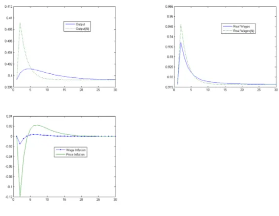
We begin by considering the response of a small open economy to a 1% tech-nology shock with the degree of persistence described above, when no use is made offiscal policy for stabilisation purposes, so only monetary policy is used to stabilise the economy. Figure 1 details the responses of key endogenous vari-ables to the technology shock, under discretion5_{. It is important to note that,}

in the absence of sticky wages, monetary policy could completely offset the welfare consequences of this shock by reducing interest rates in line with the increase in productivity. This would ensure that domestic and foreign demand

4_{In the small open economy case, γ =} χ

1−α+χ such thatfixing the share of government

spending requires a rescaling ofχto take account of the incentive to excessive government spending which is assumed to be eliminated within the union. In the simulations, to facilitate comparisons, wefixχat the value described above in both the open economy and EMU cases. 5_{The same shock under commitment introduces a slightly more inertial policy response,} but is qualitatively very similar and can be found in Leith and Wren-Lewis (2005b). The numerical solution of optimal policy under commitment and discretion is based on Soderlind (1999).

rises for the additional products and that the full effects of the productivity gain are captured in real wages. However, when nominal wages are also sticky it is not possible for monetary policy alone to offset the effects of the shock. Wage stickiness means that real wages are slow to rise following the positive productivity shock and, as a result, marginal costs fall initially and this means that the initial jump in inflation is negative. This leads to a cut in nominal interest rates (greater than that implied by the productivity shock’s affect on the natural interest rate) and a jump depreciation of the nominal exchange rate, although interest rates will be relatively lower after this initial jump as rising marginal costs increase inflation. The terms of trade depreciate initially, but this is far more modest than in theflexible wage case. As a result consumption rises in the home country relative to abroad, but not by as much as output since the depreciation of the terms of trade makes domestic goods attractive to foreign consumers. Implicitly IRS and the positive productivity shock imply that resources are being sent abroad to support foreign consumption, although this is not as pronounced as in theflexible wage case.

We know from our derivation of optimal policy above that when we utilise allfiscal instruments we can completely offset the impact of this shock on all welfare-relevant gap variables, implying that there is no additional welfare cost to the shock arising because of the various frictions in our economy. Essentially, the monetary instrument eliminates the impact on the output gap of the shock by cutting interest rates. This creates demand for domestically produced goods by encouraging domestic consumption, which has a bias towards domestically produced goods, and depreciating the exchange rate leading to an increase in foreign demand. Income taxes are reduced to eliminate wage inflation, but simultaneously achieve the required increase in the post tax real wage. The sales tax is increased to eliminate the deflation that would otherwise emerge as a result of the reduction in marginal costs (due to falling income taxes and rising productivity). There is no need to adjust government spending when the government has access to the tax instruments without constraint.

We can also consider a number of intermediate cases where not all fiscal instruments are employed. The welfare benefits of various combinations offiscal instrument are given in Table 16_{. These suggest that the greatest gains to}

stabilisation in the open economy case come from the tax instruments, with only relatively minor benefits from varying government spending. Either tax instrument is highly effective in reducing the welfare costs of the technology shock.

Table 1 - Costs of Technology Shock in Small Open Economy with Alterna-tive Fiscal Instruments.

6_{Thefigures in Tables 1-2 and 4 capture the costs of deviating from the efficient level of} variables due to sticky-wages and prices in the face of the particular shock, expressed as a percentage of one-period’s steady-state consumption. In Table 3 thefigures are a percentage of every period’s steady-state consumption.

No Taxes Income Tax Sales Tax Both Taxes Commitment Policy Govt Spending 0.5793 0.0673 0.0863 0 No Govt Spending 0.5804 0.0708 0.0915 0 Discretionary Policy Govt Spending 0.5824 0.1051 0.1356 0 No Govt Spending 0.5835 0.1082 0.1412 0

In Leith and Wren-Lewis (2005b) we also consider the costs of wage and price mark-up shocks. There we show that, as we might expect from the analy-sis above, such shocks can be effectively dealt with with the appropriate tax instruments, but the inappropriate fiscal instrument does little to offset these mark-up shocks.

5.2

EMU Simulations

We now consider the response to an idiosyncratic technology shock for a country operating under EMU (see Figure 2). We begin by considering the case where there is nofiscal response to the shock. In this case the equilibriating mechanism is the need to restore competitiveness following the shock. Relative to the small open economy case, there is now no monetary policy response to either the local productivity shock or its inflationary repercussions. As a result there is no attempt to boost consumption and output with a fall in interest rates in response to the shock (in an attempt to replicate theflex price outcome). There is an initial fall in marginal costs and inflation which induces a depreciation in the terms of trade, although this is far smaller than in the open economy case above. This shifts demand towards domestic goods such that prices and wages rise until the competitiveness gain has been reversed. In the presence of nominal inertia and with no monetary policy/exchange rate instrument, it is difficult to induce the necessary movements in the terms of trade/real exchange rate to create a market for the extra goods that can be produced as a result of the productivity shock. This failure is reflected in the large negative output gap and real wage gap.

We then contrast this to the case where country i employs all thefiscal in-struments at its disposal in Figure 37_{. We find that optimal policy attempts}

to reduce the impact of the technology shock on competitiveness. Therefore, following the technology shock, sales and income taxes are increased. The latter completely offsets the impact of the shock on wage inflation, while the former al-lows for only a very limited reduction in prices following the productivity shock. As a result of this attempt to avoid price adjustment, there is a substantial negative output gap, although this is partially offset by a rise in government spending. This has the advantage of creating a market for the additional goods, which given complete home bias in government spending, boosts real wages and

7_{Figure 3 also considers the use offiscal instruments when there are no lump-sum taxes} available to balance the budget following shocks. For a discussion of this case, see Section 6 below.

moderates the fall in inflation. There is now a smaller depreciation of the terms of trade due to the changes in taxation and the increase in government spend-ing. As we note below, the welfare gain fromfiscal stabilisation to this degree is an approximate halving of the costs of a technology shock when part of a monetary union.

We again consider a number of intermediate cases where not all fiscal in-struments are employed. The welfare benefits of various combinations of fiscal instrument are given in Table 2. This suggests that the greatest gains to stabil-isation, when part of monetary union, come from utilising government spending as a stabilisation instrument. This is due to the assumed home-bias in gov-ernment spending which allows policy makers to purchase the additional goods produced as a result of the productivity shock without requiring any competive-ness changes which subsequently have to be undone once the shock has passed. It is also interesting to note that even with all fiscal instruments in place the costs of the shock under EMU are still greater than in the small open economy case with just monetary policy as the only available policy instrument.

Table 2- Costs of Technology Shock Under EMU with Alternative Fiscal Instru-ments8_.

Commitment Policy No Taxes Income Tax Sales Tax Both Taxes Govt Spending 1.6707 1.6050 1.2089 1.1486 No Govt Spending 2.3121 2.1495 1.9988 1.8487 Discretionary Policy No Taxes Income Tax Sales Tax Both Taxes Govt Spending 1.6755 1.6115 1.2131 1.1486 No Govt Spending 2.3121 2.1537 2.0073 1.8487

The above Table shows the costs of our 1% autocorrelated technology shock, expressed as a percentage of one-period’s steady-state consumption.What would be the equivalent numbers for an historically representative set of shocks, rather than a 1% technology shock? Smets and Wouters (2005) have estimated the stochastic properties of shocks hitting the complete Euro area. We focus on three of these shocks: namely price and wage mark-up shocks which are taken to be iid shocks, and an autocorrelated productivity shock. If we subject our model of a small open economy to these shocks, wefind that the gains from optimalfiscal stabilisation (compared to nofiscal action) are 2.4% of steady state consumption. Making the even more heroic assumption that these shocks can be applied to our model of an individual union member, wefind that optimalfiscal stabilisation reduces their costs from 2.9% to 1.9% of steady-state consumption (for details of these calculations see Leith and Wren-Lewis (2005b))- see Table 3.

8_{Thefigures in Table 2 capture the costs of deviating from the efficient level of variables} due to sticky-wages and prices in the face of the particular shock, expressed as a percentage of one-period’s steady-state consumption.

Table 3 - Benefits of Fiscal Stabilisation9

Benefits of Fiscal Stabilisation No Fiscal Response Full Fiscal Response

Small Open Economy 2.37% 0%

Monetary Union 3.91% 1.90%

5.3

Implementation Lags

A frequently cited argument against employing fiscal instruments in a stabil-isation role is that it often takes long periods to implement the tax changes and government spending changes suggested by optimal policy. In this sub-section we assess the extent to which implementation lags affect the welfare gains fromfiscal stabilisation. We assume that it takes n-periods to change pol-icy instruments following a change in the information set. This can be modelled by conditioning policy instruments on information sets of n-periods ago, such that our structural model can be written as follows, with our NKPC for wage inflation,

πw_i,t=βEtπwi,t+1+eλw((1 +ϕ)yti,g−Et−ngi,gt −rw i,g

t −Et−nln(1−τit)g+u i,w t )

(131) the similar expression for price inflation,

πi,t=βEt{πi,t+1}+λ[rwti,g−Et−nln(1−τi,st )g+u i,p

t ] (132)

and the euler equation for consumption,

y_ti,g=Et−ngti,g+Et{yti+1−Et−ngti+1+πi,t+1}−(rt−ri,nt ) (133)

The equation describing the evolution of the ‘gapped’ real wage is unaffected. This implies that it will take n-periods following the shock for thefiscal author-ities to be able to implement a fiscal policy plan. In assessing the impact on such implementation lags on welfare we consider four cases: (1) There are no lags in adjustingfiscal instruments; (2) there is a one period lag in adjusting tax instruments and 2 periods in adjusting government spending; (3) there is a two period lag in adjusting tax instruments and a one year lag in adjusting government spending; and (4)fiscal instruments are not changed over the course of the business cycle.

In Table 4 below we look at these four cases for a currency union member. It is clear that implementation lags do reduce the effectiveness offiscal instruments as stabilisation devices. However, there are still non-trivial benefits from fiscal stabilisation even under the ‘slow response’ scenario. This is in part because expectations that instruments will change in the future will impact on private sector decisions today in a forward looking model.

9_{The figures in Table 3 capture the expected costs of deviating from the efficient level} of variables due to sticky-wages and prices in the face of ongoing shocks, expressed as a percentage of steady-state consumption.

Table 4: Implementation Lags10 Inertia (1) No Delay (2) Moderate Response (3) Slow Response (4) No Response ρ_a= 0.6 1.1485 1.8770 2.0451 2.3121 ρ_a= 0.9 2.6735 3.5055 4.0023 5.3955 Of course these results are highly dependent upon the amount of inertia in the economy. For example, the table shows that increasing the degree of presistence in the technology shock from 0.6 to 0.9 such that the impacts of shocks are felt for longer, implies that even with implementation lags fiscal policy has a valuable role to play in stabilising the economy. Overall, these results show the potential value of any measures that can be taken to reduce implementation lags forfiscal instruments.11

6

Introducing Debt

In this section we consider the impact of introducing government debt into our analysis of policy within a small open economy or within EMU12_{. Until}

now we have assumed that there was a lump-sum tax instrument which was utilised to balance the budget whenever otherfiscal instruments were used in a stabilisation role. In this section we assume that any variations in government spending or our sales or income tax instruments are not paid for in this way. Instead, any inconsistency between government tax revenues and spending will affect government debt. Policy must then ensure that the relevant intertemporal government budget constraint is satisfied.

In the case of EMU, Leith and Wren-Lewis (2005b) derive the intertemporal budget constraint for the union as a whole,

Z Di tdi=Rt−1Bt−1=− ∞ X T=t Et[Qt,T( Z 1 0 (Pi,TGiT−WTiNTi(τiT−κi)−τ i,s T Pi,TYTi−TTi)di)] (134) whereBtis the aggregate level of the national debt stocks. With global market

clearing in asset markets the series of national budget constraints imply that the only public-sector intertemporal budget constraint in our model is a union-wide constraint. What is the intuition for this? Given complete capital markets and our assumed initial conditions (zero net foreign assets and identicalex ante

structures in each economy) this means that initially consumers expect similar

fiscal policy regimes in their respective economies. To the extent that ex post

1 0_{These are expressed as percentages of one period’s steady-state consumption.}

1 1_{This may be easier when lags are operational rather than political. However, in the} UK in the 1960s, whenfiscal policy was actively used in demand management, the so called ‘regulator’ set aside sales taxes that could be changed by the government without the need to obtain parliamentary approval, so as to reduce these lags.

1 2_{In Leith and Wren-Lewis (2005c), we consider more fully the significance of adding debt} to New Keynesian models of monetary policy.

this is not the case, there will be state contingent payments under IRS that ensure marginal utilities are equated throughout the union (after controlling for real exchange rate differences)13_{. This would seem to suggest that fiscal}

sustainability questions within this framework are a union-wide rather than a national concern. Given that a national government’s contribution to union-widefinances is negligible then this could be taken to imply that debt is not an issue in utilisingfiscal instruments at the national level within EMU.

However, given the fiscal institutions which have been constructed as part of EMU, it seems unlikely that without such constraints each member state would expect to operate underex ante similarfiscal regimes. Therefore it may be reasonable to assume that each member state operates a budget constraint of this form at the national level, such that there is no need for the only insti-tution with a union-wide instrument, the ECB, to be concerned with issues of

fiscal solvency. Therefore we impose, as an external constraint created within the institutions of EMU, a national government budget constraint of the same form. We also need to transform this ‘national’ budget constraint into a log-linearised ‘gap’ equation to allow it to be integrated into our policy problem. Additionally, in order to support the assumption that the steady-state level of output was efficient (which was implicit in the welfare functions we developed) an obvious assumption to make is that lump-sum taxation is used tofinance the steady-state subsidy (which offsets, in steady-state, the distortions caused by distortionary taxation and imperfect competition in wage and price setting). We shall then assume that lump-sum taxation cannot be used to alter this subsidy or to finance any other government activities, including the kind of spending and distortionary tax adjustments as stabilisation measures we are interested in. This implies thatWi

TNTiκi=TTi in all our economies at all points in time,

allowing us to simplify the budget constraint to,

Rt−1Bti−1=− ∞ X T=t Et[Qt,T(Pi,TGiT −WTiNTiτiT −τ i,s T Pi,TYTi)] (135)

i.e. distortionary taxation and spending adjustments are required to service government debt as well as stabilise the economy. This defines the basic trade-offfacing policy makers in utilising these instruments.

Leith and Wren-Lewis (2005b) show that this intertemporal budget con-straint can give rise to log-linearisedflow dynamics of,

bi_t = Rbi_t−1+R(rt−1−πi,t) + Gi BilnG i t+ (1₋τi,s_)Yi Bi ln(1−τ i,s t )(136) −τ i,s_Yi Bi y_ti+(1−τ i_)rwi_Ni Bi ln(1₋τi_t)₋τrw i_Ni B/Pi (rw_ti+ni_t)

1 3_{For the purposes of illustration, suppose taxes were lump-sum and one economy} unexpect-edly cut all taxes to zero. There would be transfers from this economy to the other economies to ensure that the consumers in the other economies were not disadvantaged by the higher taxes they had to pay to ensure union-wide solvency.

−RlnBi₋R(r)₋G i Bi lnGi₋(1−τ i,s_)Yi bi ln(1₋τi_t) −τ i,s_Yi Bi Y i +(1−τ i_)rwi_Ni Bi ln(1−τ i₎ −τ i_rwi_Ni Bi (rw i_+ni₎ wherebi t= ln( Bti Pi,t)andB i = (Bi_/P

i).Which can be re-written in gap form,

bi,g_t = Rbi,g_t−1+R(rg_t−1−πi,t) +

Gi Bi 1₋γi,n γi,n g i,g t + (1₋τi,s_)Yi Bi ln(1₋τi,s_t )g −(R₋1)y_ti,g+(1−τ i_)rwi_Ni Bi ln(1−τ i t)g− τrwiNi Bi (rw i,g t ) (137)

This is our national government budget constraint, which must remain station-ary as an additional constraint on policy makers.

6.1

Optimal Precommitment Policy with Government Debt

6.1.1 Small Open Economy Case

The Lagrangian associated with the open economy case in the presence of a national government budget constraint is given by,

Lt = ∞ X t=0 βt[² λπ 2 i,t+ ²w e λw(π w i,t)2+ (yi,gt )2(1 +ϕ) + 1 χ(g i,g t )2

+λπ_tw,i(πw_i,t−βEtπwi,t+1−λew((1 +ϕ)yti,g−g i,g t −(rw i,g t )−ln(1−τit)g) +u i,w t )

+λπ_t,i(πi,t−βEt{πi,t+1}−λ[rwi,gt −ln(1−τ i,s t )g+u

i,p t ])

+λy,it (yti,g−gti,g−Et{yti,g+1−g

i,g

t+1+πi,t+1}+ (rti−ri,nt ))

+λrw,i_t (rwi,g_{t −}πw_i,t+πi,t₋rwi,g_t−1+∆ai_t)

+λb,i_t (bi,g_{t −}Rbi,g_t−1−R(ri,g_t−1−πi,t)−bggti,g−bτsln(1−τi,s_t )g +byyti,g−bτln(1−τit)g+brwrwti,g)] wherebg= G i Bi 1−γi,n γi,n ,bτs = (1−τ i,s_)Yi Bi ,by =R−1,bτ = (1−τi_)rwi_Ni Bi , andbrw = τrwi_Ni

Bi . The foc for the national interest rate is given by,

λy,i_{t −}Etλb,i_t+1 = 0 (138) Here monetary policy must now take account of its impact on the government’s

finances.

In terms of national focs, we begin with the foc for the sales tax gap,ln(1₋

τi,s₎g_,

Similarly, the condition for income taxes is given by,

e

λwλπ

w_,i

t −bτλb,it = 0 (140)

and for real wages,

−λλπ_t,i+λewλπ w_,i t +λ rw,i t −βλ rw,i t+1 +brwλb,it = 0 (141)

The remainingfirst-order conditions are for debt,

λb,i_{t −}βRλb,i_t+1= 0 (142) which implies that,E0λb,it =λb,i ∀t . In other words policy must ensure that

the ‘cost’ of the government’s budget constraint is constant following a shock, which is the basis of the random walk result of Schmitt-Grohe and Uribe (2004). This also implies that the lagrange multipliers for the wage and price phillips curves are constant over time too. The remaining focs are for inflation,

2² λπi,t+λ π,i t −λ π,i t−1−β− 1

λy,i_t−1+λrw,i_t +Rλb,i_t = 0 (143)

wage inflation,

2²w

e

λw

π_i,tw +λπ_tw,i₋λ_tπ₋w₁,i₋λrw,i_t = 0 (144) the government spending gap,

2 χg i,g t +λewλπ w_,i t −λ y,i t +β−1λ y,i t−1−bgλb,it = 0 (145)

and the output gap,

2(1 +ϕ)y_ti,g₋eλw(1 +ϕ)λπ w_,i t +λ y,i t −β−1λ y,i t−1+byλb,it = 0 (146)

Combinations of thesefirst order conditions define the national target criteria for a variety of cases. In the open economy case the optimal combination of wage and price inflation is given by,

2² λπi,t+ 2²w e λw πw_i,t= 0 (147) This essentially describes the balance between wage and price adjustment in achieving the new steady-state real wage consistent with the new steady-state tax rates required to stabilise the debt stock following the shock. Taking the foc for the output gap, we have,

2(1 +ϕ)y_ti,g+λb,i(₋bτ(1 +ϕ) + (1−β−1) +by) = 0 (148)

which defines the value of the Lagrange multiplier associated with the govern-ment’s budget constraint which implies that the output gap is constant, but

non-zero. The sales and income tax rules for the open economy case are given by, respectively,

−2²(rwi,gt −ln(1−τi,st )g+ui,pt ) + (brw+bτ−bτs)λb,i= 0 (149)

and, 2²w((1+ϕ)yti,g−g i,g t −rw i,g t −ln(1−τit)g)+u i,w t )+(brw+bτ−bτs)λb,i= 0 (150)

Finally the government spending rule is given by, 2

χg i,g

t + (bτ−(1−β−1)−bg)λb,i= 0 (151)

which is again constant given the lagrange multiplier λb,i . Leith and Wren-Lewis (2005c) show that this lagrange multiplier, associated with the budget constraint, can be solved as a function of the size of the initial debt stock and the expectedfiscal repercussions of any modelled shock. They also investigate the nature of the time inconsistency problem inherent in adding debt to the model, which is discussed in the simulation section below.

Taken together these target criteria imply that optimal policy ensures that output and government spending adjust instantaneously to their new steady-state levels, while gradual price and wage adjustment implies that it is optimal, under commitment, to gradually reach the new steady-state tax rates consistent with debt sustainability.

6.1.2 EMU Case

If we formulate the corresponding problem for the EMU case we have,

Lt = Z 1 0 ∞ X t=0 βt[² λπ 2 i,t+ ²w e λw (πw_i,t)2+ (yi,g_t )2(1 +ϕ) + 1 χ(g i,g t )2

+λπ_tw,i(πw_i,t−βEtπw_i,t+1−λwe ((1 +ϕ)y_ti,g₋gi,g_{t −}rw_ti,g₋ln(1₋τi_t)g+ui,w_t ) +λπ_t,i(πi,t₋βEt{πi,t+1}−λ[rwi,gt −ln(1−τ

i,s t )g+u

i,p t ])

+λy,i_t (y_ti,g₋g_ti,g₋Et{yti,g+1−g

i,g

t+1+πi,t+1}+ (rt−ri,nt ))

+λrw,i_t (rwi,g_{t −}πw_i,t+πi,t−rwi,gt−1+∆ait)

+λb,it (bi,gt −Rbi,gt−1−R(r

g

t−1−πi,t)−bggti,g−bτsln(1−τi,s_t )g +byyti,g−bτln(1−τit)g+brwrwti,g)]di

In order to obtain intuition for optimal policy in this case it is helpful to relate the (constant) value of the lagrange multiplier associated with the na-tional government budget constraint to nana-tional output and government spend-ing gaps,

2(1 +ϕ)yi,g_t + 2

χg i,g