Benchmark Problems and Performance Indicators
for Search of Knee Points in Multi-objective
Optimization
Guo Yu,
Student Member, IEEE,
Yaochu Jin,
Fellow, IEEE,
and Markus Olhofer
Abstract—In multi-objective optimization, it is non-trivial for decision makers to articulate preferences withouta priori knowl-edge, which is particular true when the number of objectives be-comes large. Depending on the shape of the Pareto front, optimal solutions such as knee points may be of interest. Although several multi- and many-objective optimization test suites have been proposed, little work has been reported focusing on designing multi-objective problems whose Pareto front contains complex knee regions. Likewise, few performance indicators dedicated to evaluating an algorithm’s ability of accurately locating all knee points in high-dimensional objective space have been suggested. This paper proposes a set of multi-objective optimization test problems whose Pareto front consists of complex knee regions, aiming to assess the capability of evolutionary algorithms to accurately identify all knee points. Various features related to knee points have been taken into account in designing the test problems, including symmetry, differentiability, degeneration. These features are also combined with other challenges in solving optimization problems, such as multimodality, linkage between decision variables, non-uniformity and scalability of the Pareto front. The proposed test problems are scalable to both decision and objective spaces. Accordingly, new performance indicators are suggested for evaluating the capability of optimization algo-rithms in locating the knee points. The proposed test problems together with the performance indicators offer a new means to develop and assess preference-based evolutionary algorithms for solving multi- and many-objective optimization problems.
Index Terms—Benchmark problems, performance indicators, knee points, knee regions, multi-objective optimization.
I. INTRODUCTION
M
ULTIOBJECTIVE optimization problems (MOPs) in-volve multiple conflicting objectives, which can be defined as follows:min
x :z(x) = (f1(x),· · ·, fm(x))
subject tox∈Ω (1)
wherex= (x1,· · ·, xn)∈Ωis the decision vector.Ω⊆Rnis the decision space, andnis the number of variables.z: Ω→
Rm denotes the objective vector consisting ofm real-valued objectives. MOPs having more than three objectives are also known as many-objective optimization problems (MaOPs) [1], [2].
Guo Yu and Yaochu Jin are with the Department of Computer Sci-ence, University of Surrey, Guildford, Surrey GU2 7XH, UK. e-mail: (guo.yu; yaochu.jin)@surrey.ac.uk. (Corresponding author: Yaochu Jin)
Markus Olhofer is with Honda Research Institute Europe GmbH, Carl-Leigien-Strasse 30, D-637073 offenbach/Main, Germany. e-mail: [email protected].
Over the last decades, many algorithms have been devel-oped both in the multiple criteria decision making (MCDM) community and the evolutionary computation community that are capable of finding a set of well-distributed solutions approximating the Pareto optimal front (PoF). Earlier popular multi-objective evolutionary algorithms (MOEAs) for dealing with MOPs are mainly dominance based, include NSGA-II [3], SPEA2 [4], NPGA [5] and PESA [6]. Although dominance based MOEAs work well for MOPs, their efficiency seriously degrades as the number of objectives increases [7]. Conse-quently, a large body of research in evolutionary optimization has been dedicated to solving MaOPs over the past few years. MOEAs for MaOPs can roughly be divided into four cate-gories [8], [9], namely, dominance relationship modification based methods [10]–[13], indicators based methods [14]–[16], aggregation based (also known as decomposition based) [17]– [19] or preference based approaches [20]–[23]. There are also methods which do not belong to the above three categories, such as the objective reduction [24], the shift-based density estimation [25], the two-archive strategy [26], the boundary elimination selection [27] and the knee-point driven MOEAs [28].
While considerable progresses have been made in research on MaOPs, some challenges remain to be addressed. For example, it will be impractical to represent the entire Pareto front in a high-dimensional objective space using a relatively small number of solutions. In addition, it becomes increasingly challenging to select preferred solutions from the obtained solution set. Furthermore, preference articulation will be more difficult for MaOPs. Last but not the least, most performance indicators measuring the distribution of solutions no longer work properly in high-dimensional objective space since it is computationally extremely intensive to densely sample a high-dimensional space.
Due to the difficulties discussed above, it is more practical to concentrate on potentially interesting regions in solving MaOPs. To this end, preference driven MOEAs provide an effective means to focus on the search of solutions of interest [29] and are computationally more efficient [22], [30].
Preference based optimization approaches can be classified into three groups, i.e., a priori, interactive, and a posteriori
methods, according to the time when the decision-maker’s preferences are embedded during the search process. Detailed discussions about the incorporation of user preferences into multi-criterion decision-making and analysis can be found in [31], [32].
Among various user preferences, geometric properties of the Pareto front (PoF) are considered to be natural and generic user preferences [33]. For instance, knee points on the Pareto front are most preferred since for solutions near the knee points, gaining a small amount in one objective requires an unfavorably large sacrifice in other objectives [34]–[36]. Different interpretation of knee points can also be found in [37], [38].
Many methods have been proposed to find knee points by using, e.g., the reflex angle [39], extended angle dominance [40], [41], expected marginal utility [42], [43], distance-based strategy [34], [38], and the ratio between the improvement and deterioration when exchanging the objectives of two solutions [37], and the niching-based method [44]. However, few benchmark problems have been designed to systematically assess the ability of an optimization algorithm to find knee points with few exceptions, including the DO-DK and DEB-DK problems [42], [45]. Note that DO-DEB-DK and DEB-DEB-DK problems are designed only for identifying knee points without considering many important characteristics of knee points such as the positions of the knees, different geometric shapes of the PoF, bias, separability, degeneration of the knee regions, differentiability of the knees, scalability of the PoF, and symmetry of the knee regions.
This work is motivated by the fact that few knee functions, benchmark problems and performance indicators have been proposed to test and assess the performance of MOEAs in approximating knee points of multi- and many-objective opti-mization problems in terms of the number of the knee points found, their accuracy and location. To fill the gap, we propose five new basic knee functions and a new construction method of knee functions. Furthermore, a set of new benchmark problems are constructed using the proposed knee functions whose Pareto fronts have various characteristics in symmetry, differentiability and degeneration. Apart from these properties directly related to knee regions, other challenges in solving optimization problems such as multi-modality, non-uniformity and linkage in decision variables are taken into account. Mean-while, performance indicators for evaluating various aspects related to MOEAs’ performance in identification of knee points of complex Pareto fronts are suggested.
The rest of the paper is organized as follows. Section II pro-vides a concise review of existing benchmark problems. Sec-tion III elaborates various features of Pareto optimal soluSec-tions considered in construction of the test problems. Section IV presents the details for constructing the proposed benchmark problems, followed by a description of the proposed metrics in Section V. The experiments and analysis are conducted in Section VI. Finally, Section VII concludes the paper.
II. RELATED WORK
In this section, we briefly review existing popular bench-mark problems based on which this work is built.
A. ZDT and DTLZ problems
The ZDT [46] and DTLZ [47] test suites are most widely used multi-objective optimization benchmark problems con-structed for evaluating MOEAs. The construction of both test
suites is based on the bottom-up approach [47], which allows for separately design of the objective functions, the decision space, and the Pareto-optimal front. Specifically, decision variables are divided into position and distance variables, which define the Pareto front and determine the distance of the solutions to the PoF, respectively. The ZDT test suite is constructed in the following form:
min
x :z(x) = (f1(x1), f2(x))
subject tof2(x) =g(x2,· · ·, xn)h(f1(x1), g(x2,· · · , xn)) wherex= (x1,· · ·, xn)∈Ω
(2) In the above construction, x1 is the position variable and
the rest are the distance variables. The ZDT test problems are constructed using three basic functions, namely, the po-sition/distribution function f1 with or without bias for
con-trolling the distribution of Pareto optimal solutions along the PoF, the uni- or multi-modal distance function g for testing the algorithm’s ability of converging to the PoF, and the shape functionhfor determining the convexity and continuity of the PoF.
The DTLZ test suite [47] was developed based on the ZDT test functions in order to enhance the scalability to the number of decision variables and objectives. The DTLZ test suite is constructed as follows: min X :fi=1:m(X) = (1 +g(XII))·hi(XI). whereX = (XI, XII)∈Ω XI = (x1,· · ·, xm−1), XII = (xm−1,· · · , xn) (3)
where, XI in the shape functions h1:m(XI) are the position variables determining the geometry of the PoF whileXII are the distance variables embedded in the landscape functions to control the closeness of the Pareto optimal solutions to the PoF, where mis the number of objectives.
Note, however, that neither ZDT nor DTLZ pays particular attention to the complexity of the PoF, and it is assumed that there is no correlation between the position and distance variables.
B. WFG problems
The design of the WFG problems [48], [49] also follows the bottom-up approach [47] but differs from the approach to designing the ZDT and DTLZ test suites. The construction of the WFG test suite is as follows:
Givenz={z1,· · ·, zk, zk+1,· · ·, zn} min x :fi=1:m(x) =xm+Sihi(x1,· · · , xm−1) x={x1,· · · , xm}={max(tpm, A1)(t p 1−0.5) + 0.5, · · ·,max(tpm, Am−1)(tpm−1−0.5) + 0.5, t p m} tp ={tp1,· · ·, tpm} ←[tp−1←[· · · ←[t1←[z[0,1] z[0,1]={z1,[0,1], . . . , zn,[0,1]}={z1/z1,max, · · ·, zn/zn,max} (4)
The WFG test suite is used for constructing a problem in terms of an underlying vector of decision variables xderived
from a series of transition vectors t1:p, where the transition vectors are derived from a vector of working parameters z. Each transition vector can add complexity to the underlying test problem, such as non-separability, multimodality, decep-tion, and bias. S1:m > 0 and A1:m−1 ∈ {0,1} are scaling
and degeneracy constants, respectively. Thus, a benchmark problem can be created from different combinations of the shape functionsh1:mdefining the geometry of the fitness space and a number of transformation functions ‘←[’ determining the searching space.
One unique property of the WFG test suite [48], [49] is that the Pareto front of the test problems can be specified, similar to the idea reported in [50]. Like the ZDT and DTLZ test suites, the WFG test suite does not pay special attention to the design of knee regions on the PoF.
C. DO-DK and DEB-DK problems
Knee points are an important geometric feature on the PoF, where it requires an unfavorably large sacrifice in one objective to gain a small amount in other objectives. Without any specific user preferences about the Pareto optimal solutions, knee points are naturally preferred solutions. More detailed discussions about knee points are given in Section III.
Due to potential importance of the knee points, test prob-lems such as DO-DK and DEB-DK have also been designed by embedding the desired knee points following the bottom-up approach [47]. The construction of the DO-DK [42] and DEB-DK [45] problems is as follows:
min
X :fi=1:m(X) =g(XII)r(XI)hi(XI). whereX = (XI, XII)∈Ω
XI = (x1,· · ·, xm−1), XII = (xm−1,· · ·, xn) (5)
where r(XI)are the knee functions that can create different geometries of the PoF. However, only one knee function is designed in the DO-DK and DEB-DK problems and they are not able to specify detailed features of the knee regions such as differentiability, degeneration, and symmetry or asym-metry. Another limitation is that features that can challenge MOEAs’ convergence ability is not considered, such as multi-modality in the fitness landscape, linkage between the decision variables, and non-uniformity of the PoF. In addition, the scalability of the PoF has not been considered.
This work aims to design multi- and many-objective opti-mization test problems that can systematically challenge and evaluate MOEAs’ ability of accurately identifying knee points. For this purpose, most “hardness” aspects for MOEAs that can be seen in the real-world are considered and integrated into the benchmark problems. The proposed test problems are scalable in the decision space, the objective space, and the true PoF. Furthermore, the true location and number of knee points are known, which is an important requirement for designing benchmark problems.
III. GENERICALLYPREFERREDSOLUTIONS
Generally speaking, knee points, edge knee points, extreme points, and robust solutions [39], [51] are solutions generically
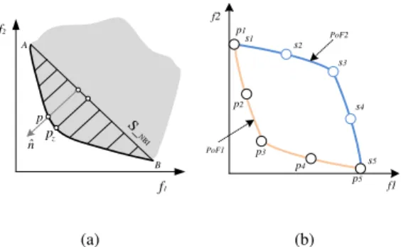
f1 f2 A B ˆ n S_N BI p z p f1 f2 p1 p2 p3 p4 p5 s1 s2 s3 s4 s5 PoF1 PoF2 (a) (b)
Fig. 1. (a) Identify the knee point in convex region using NBI method. (b) differentiate the knee points in convex and concave region by an utility function.
TABLE I
AN EXAMPLE OF KNEE POINT IN THE CONVEX REGION ACCORDING TO DEFINITION5. τ(, p1) τ(, p2) τ(, p3) τ(, p4) τ(, p5) min p1: (1,11) - 1/4 1/4 2/3 1 1/4 p2: (2, 7) 4 - 1/4 1 3/2 1/4 p3: (3, 3) 4 4 - 4 4 4 p4: (7, 2) 3/2 1 1/4 - 4 1/4 p5: (11,1) 1 2/3 1/4 1/4 - 1/4
preferred by users. In the following, we discuss in detail the main properties of knee points and knee regions before we design the benchmark problems.
A. Knee points
Knee points, which require large sacrifices in at least one objective to gain a small amount of improvement in another objective [36], [39], can be largely divided into three cate-gories, i.e., knees in convex regions, knees in concave regions, and edge-knees.
1) Knees in convex regions: Multiple definitions for knee
points have been given in the literature [36]. We discuss here two of them in the following.
Definition 1In [34], Das indicates that the knees correspond
to the local maxima in terms of the distance from the convex hull of individual minima (CHIM) measured along the normal to the CHIM.
In the normalized coordinate system, as shown in Fig. 1 (a), the knee pointpz= arg max
pi
(|ti|· kˆnk), where ˆnis the orthogonal basis of the boundary lineS_N BI, and |ti| is the distance from normalized solutionpi toS_N BI.
Definition 2In [37], the knee in the convex region is
char-acterized by the maximum utility, namely,arg max
pi (µ(pi, P)), where µ(pi, P) = min i6=j,pi⊀pj,pj⊀pi τ(pi, pj), and τ(pi, pj) = P 1<ι<mmax[0,fι(pj)−fι(pi)] P
1<ι<mmax[0,fι(pi)−fι(pj)], andmis the number of objectives.
In the definition ofτ(pi, pj), the numerator and denominator are the aggregation of the deterioration and improvement in the exchange of the objectives, respectively. In Fig. 1 (b), p1
top5 are on the PoF1, and their coordinates and utilities are presented in Table I. Obviously, knee pointp3is the one with
max−min utility value.
2) Knees in concave regions: Little work has been reported
TABLE II
AN EXAMPLE OF KNEE POINT IN CONCAVE REGION ACCORDING TO DEFINITION6. τ(, s1) τ(, s2) τ(, s3) τ(, s4) τ(, s5) max s1: (1,11) - 4 4 3/2 1 4 s2: (5,10) 1/4 - 4 1 2/3 4 s3: (9, 9) 1/4 1/4 - 1/4 1/4 1/4 s4: (10,5) 2/3 1 4 - 1/4 4 s5: (11,1) 1 3/2 4 4 - 4 gain sacrifice f1 f2 f1 f2 gain sa cr if ic e Edge-knee Edge-knee region A B
Fig. 2. Two examples for edge-knees.
Pareto front with few exceptions [36], [43]. We consider it also of interest to find these solutions for the following reasons, in particular when the number of objectives is large.
First, it is challenging to identify knee solutions in high-dimensional spaces, although it is relatively straightforward either visually or mathematically to identify knee solutions in two- or three-objective optimization problems. It is interesting to note that there is usually a convex knee region between two concave knee regions, or the other way around. Thus, solutions in concave regions might be helpful for finding knees in convex regions. Second, the knees in concave regions, together with those in convex regions, will be able to provide the user with a better structure information of the whole Pareto front in a high-dimensional space, thereby helping the user to articulate preferences more effectively.
Definition 3 The knee in the concave region is
charac-terized by the minimum utility, namely, arg min
pi (µ(pi, P)), where µ(pi, P) = max i6=j,pi⊀pj,pj⊀pi τ(pi, pj), and τ(pi, pj) = P 1<ι<mmax[0,fι(pj)−fι(pi)] P
1<ι<mmax[0,fι(pi)−fι(pj)], andmis the number of objectives.
In Fig. 1 (b), s1-s5 are non-dominated solutions on PoF2. After a pairwise comparison,s3is identified as the knee with the min−maxutility value.
3) Edge knee points: In [39], an edge knee point is defined
in a two-dimensional objective space. They are preferred in case the knee point has an unfavorably large compromise on only one side of the point, and no solutions other than an extreme point1 can be chosen.
Definition 4In [39], a Pareto optimal solution is defined as
aγ-edge-knee point if it lies near an extreme point and a unit gain in one of the objective functions would require at least an amount of sacrifice γin the other objective function.
1Given a finite population P, ∀y ∈ P, ∃i ∈ {1,· · ·, m}, x =
arg max x fi(y), and∀j∈ {1,· · ·, i−1, i+ 1,· · ·, m}, fj(x) = minfj(y). 0 2 4 6 8 0 2 4 6 8 PoF 0 2 4 6 8 0 2 4 6 8 PoF Reference point (a) (b)
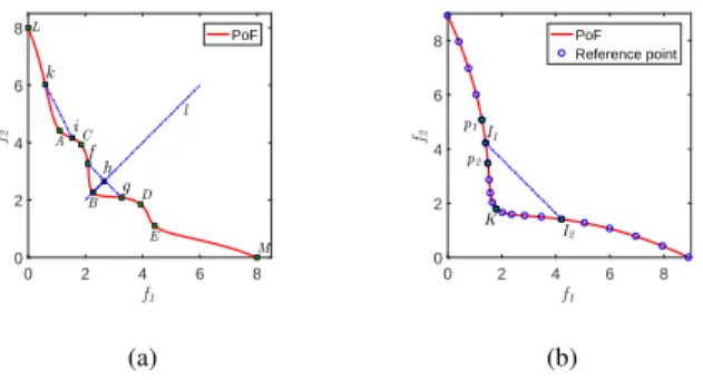
Fig. 3. (a) An illustrative example of characters of knee regions. (b) An illustrative example how to mathematically calculate the width.
In Fig. 2, _
ABis aγ-edge-knee region where a large sacrifice in objectivef1is needed for a small gain in f2.
B. Characteristics of knee regions
Although much work has been done to find knee points, little in-depth analysis has been made on the characteristics of the regions in which the knee points are located. In the following, we provide a detailed discussion about the basic characteristics of the knee regions, including symmetry, width, depth, differentiability, and degeneration.
1) Symmetry: The symmetry of a knee region means that
the shape of the knee region is symmetric to a line or hyperplane passing through the knee point. For example, in Fig. 3 (a),
_
CD is a symmetrical convex region in that _
CB
and _
BD are symmetrical to the line f1 = f2. By contrast, the concave regions (
_
AB and
_
BE) are asymmetrical. Note that if the knee regions or the PoF are asymmetrical, it will become more difficult for some algorithms [37] to identify the knees due to the different trade-off relationships when one objective increases or decreases.
2) Width: The width of a knee region describes how large
the basin around the knee point is. In the following, we provide two quantitative definitions for the width of a knee region. It should be noted that the trade-off relationship between different objectives are usually different, and consequently, the definition of the width of a knee region in a high-dimensional objective space is not straightforward. To address this issue, we propose to define the width of a knee region to be the smallest intersection between the hyperplane S constructed by the extreme points of the PoF, and a hyperplane that is perpendicular to S and passes through the knee point. The following two possible methods can be used to determine the width of the knee region. The first idea is to calculate the distance between the two inflection points at each side of the knee point whose second derivative equals 0. For example in Fig. 3(a), pointsk,iare the two inflection points of the knee region
_
LC. The width of the convex knee region of knee point
Ais defined to be the length of lineki.
The second idea is to calculate the distance between two points on the two sides of the knee whose tangent line exactly passes the knee point. In Fig. 3 (a), for instance, pointsf andg
(a) knee function (b) PoF
Fig. 4. An example of non-differentiable knees on the PoF.
passes the knee point B. Thus, the width of the convex knee region of knee point Ais the length of the linef g.
If the width of the knee region is calculated according to the first method, there will be no overlap between two neighboring knee regions. Unfortunately, it is impractical to calculate the width of a knee region using this method since an analytic description of the PoF is unknown. By contrast, the second method is more easily applicable given a set of non-dominated solutions, since the points can be estimated by checking the relationship between the solutions.
Fig. 3 (b) provides an illustrative example, where pointKis the knee point and the circles denote a set of obtained solutions on the PoF. From the given solution set, solutions I1 and I2
can be determined to be an approximation of the two solutions for estimating the width using the second method. At first, solutions like p2 between solutions K and I1 are all below
the lineKI1, which do not satisfy the condition. However, all
solutions but I1 between K and p1 are below the lineKp1.
ThusI1 can be determined to be the solution on the left side
of knee pointKand similarly,I2is the solution on the right of
K for calculating the width of knee region ofK. By contrast, it is difficult to find the inflection points in the given solution set using the first method.
3) Depth: In [34], the knee point is characterized as
pz= arg max pi
(|ti|· kˆnk)in a normalized coordinate system, where nˆ is the orthogonal basis of the boundary line (or hyperplane)S_N BI constructed by the extreme points, and|ti| is the distance from normalized solutionpi toS_N BI.
Thus, once the width of a knee region is fixed, in terms of the above method, the depth of a knee region is the distance from the knee point to theS_N BI constructed by the boundary points obtained by the second method in Subsection III-B2. For example in Fig. 3 (a), |Bh| is the depth of the convex region of knee point B.
4) Differentiability: The differentiability of a knee region is
typically determined by the knee function used in constructing the benchmark problem. If the knee function is differentiable, the resulting knee points will also be differentiable. Otherwise, some of the knee points will be non-differentiable. In Fig. 4 (b), for example, the convex knees are located in the center of the convex regions and they are non-differentiable since the knee function in Fig. 4 (a) is not differentiable on two points.
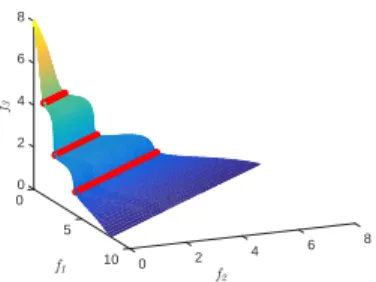
5) Degeneration: Knee regions do not always have a
trade-off relationship between all objectives. A knee region is said to be degenerate where some of the objectives do not have a trade-off relationship with others. In Fig. 5, for instance, the convex knee regions are degenerate.
0 2 0 4 6 8 5 8 6 4 2 10 0
Fig. 5. An illustrative example of the degenerated knee regions.
IV. PROPOSEDBENCHMARKPROBLEMS
As introduced in Subsection II-C, there are few benchmarks dedicated to the design of knee regions except for the ones presented in [42], [45]. However, among these benchmarks, only one specific knee function is designed, and many other features of the knee regions such as symmetry, differentiability, and degeneration of the knee regions are not accounted for. Besides, no research has been reported on the effect of the knee function on the scalability of the PoF.
Thereby, by following the bottom-up approach [46], [47] and extending the previous work [42], [45], this work aims to construct scalable multi-objective benchmark problems with a complex knee structure in terms of symmetry, differentiability, scalability and degeneration of the PoF, while still considering other complexities in problem structures [48], [52] such as multi-modality, non-uniformity, scalability of PoF and separa-bility.
In order to design benchmark problems having a complex knee structure, a mathematical construction method embed-ding knee point information can be designed as follow:
min X :fi=1:m(X) = (1 +g(`(X)))·η(k(XI))·h(XI). (6) where X = (XI, XII), and XI = (x1,· · ·, xm−1), XII = (xm,· · · , xn), andk(XI) = Qm−1 i=1 signi·k(xi) m−1 .
In the above construction, g(X)is the landscape function that controls the degree of hardness for MOEAs to converge to the PoF by means of introducing separability and multi-modality into the landscape functions. Furthermore, the hard-ness in optimizing different objectives may differ, resulting in different convergence speeds for different objectives. Here, we take this feature into account by embedding different landscape functions on different objectives.`(X)is the linkage function that can change the correlation relationship between the decision variables and shift the position of the global optima linearly or nonlinearly. The basic shape functionh(X)
determines the basic shape of the PoF such as uniformity and convexity. Non-uniformity can be introduced using a parameter inh(X). Note that the knee functionk(X)and the basic shape function h(X)together will determine the shape of the PoF.
Different from [42], [45], here we propose a new structure of the knee combinations and embed them into the stretching functions. The knee-driven stretching function η(k(X)) en-ables us not only to create different knee structures on the PoF, but also to change the scalability of the PoF. Parameters in the
TABLE III
DIFFERENT ROLE FUNCTIONS TO TEST DIFFERENT ABILITIES OF AN ALGORITHMS.
Functions Features g(X) Separability, multimodality
`(X) Linear and nonlinear shift of the optima
η(X) Scalability of the PoF k(X)
Symmetry, bias, degeneration, Scalability of the number of knees, differentiability, depth/location of the knee regions. h(X) convexity and non-uniformity.
n u l n x x R :[ , ] m u l m f f R :[ , ]
Mapping space Mapping function
I X } ,..., , ,..., {x1 xm1 xm xn x ) ( hXI )) , ( ( XI XII g 1:( ) ( ( )) h( ) (1 ( ( , )) i m I I I II f x k X X g X X II X ) , (XI XII 1 -1 sign k ( )i i i i m x ( (k XI))
Fig. 6. The mapping relationships of the proposed benchmark framework.
knee functions k(X)can be used to determine the symmetry of PoF, the number of knees, the location, degeneration as well as the differentiability of the knee regions. A parameter in k(X) can also control the bias of the PoF. The η(X)
is the stretching function, adopting different combinations of the elementary functions like power functions, exponential functions, and logarithmic functions to stretch the objectives. Table III summarizes the functions and their main roles in constructing the benchmark problems.
Fig. 6 shows the relationships between decision variables, objectives and functions η(k(X)), `(X), h(X) and g(X). A detailed description of the role of these functions will be provided in the following. The description of the landscape function g(X) and the basic shape function h(X) can be found in the Supplementary material. Note that it is very flexible to include or exclude certain aspects of hardness in the benchmark problems. For example, the knee function can be replaced by a constant 1 if no influence of the knee points is to be considered. To remove the dependencies between the decision variables, the linkage functions can be substituted by
XII. We can set the bias parameterB= 1in the knee function and p= 1 in the basic shape functions if no non-uniformity is taken into account.
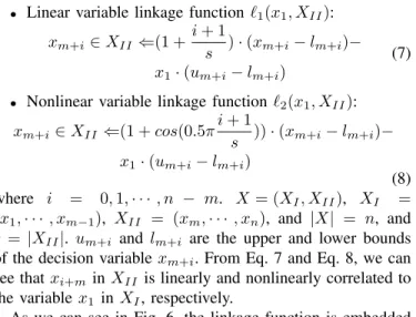
A. Linkage Functions `(X)
There is correlation between the decision variables in many real-world optimization problems. Thus the test problems proposed in this work also introduce a linkage function to simulate the dependencies between the decision variables. The linkage function will shift the position of the Pareto optimal solutions, resulting in increased difficulty in locating the PoS. Following the design principles in [52]–[54], we will adopt both linear and nonlinear linkage functions.
• Linear variable linkage function`1(x1, XII):
xm+i∈XII ⇐(1 +
i+ 1
s )·(xm+i−lm+i)− x1·(um+i−lm+i)
(7)
• Nonlinear variable linkage function`2(x1, XII):
xm+i∈XII ⇐(1 +cos(0.5π i+ 1 s ))·(xm+i−lm+i)− x1·(um+i−lm+i) (8) where i = 0,1,· · · , n − m. X = (XI, XII), XI = (x1,· · ·, xm−1), XII = (xm,· · ·, xn), and |X| = n, and
s =|XII|. um+i andlm+i are the upper and lower bounds of the decision variablexm+i. From Eq. 7 and Eq. 8, we can
see thatxi+minXII is linearly and nonlinearly correlated to the variablex1 inXI, respectively.
As we can see in Fig. 6, the linkage function is embedded in the landscape function. Thus, the optima of functiongwill be shifted since all variables inXII are dependent on the first variablex1 inXI.
B. Knee functionsk(XI)
In [42], [45], k(XI) = Pim=1−1k(xi)/(m − 1), which is a linear combination of the basic knee functions. The gradient information is kept consistent with the tendency of the line k(xi). Without considering the degeneration, this work gives a new construction of k(XI), namely, k(XI) =
Qm−1
i=1 k(xi)/(m−1). Both constructions can create similar knee features but the latter is a nonlinear combination of the basic knee functions, and creates inconsistent gradient information on the hyperplane. In Fig. 8 (b), the gradient of the blue dashed lines has prominent changes in the four corners but there is less information in the center area, compared with the red contour lines. It indicates that the newly proposed construction method can create more difficulties for an algorithm to detect the knee regions, since the optimizer may get trapped in the regions with large variations of the gradient information.
Thus, in this paper,k(XI)can be defined as follows: k(XI) =
Qm−1
i=1 signi·k(xi)
m−1 (9)
whereXI = (x1,· · · , xm−1), andk(x)is the basic knee
func-tion. In each problem,k(XI)is only correlated with one cer-tain basic knee function, for example,k(XI) =
Qm−1
i=1 k1(xi)
m−1 .
In this work, the following six basic knee functions have been used. Note that sign = {0,1}|m−1| controls whether |m−1|variables are included in the knee functions. In other words,signi= 1if there is no degeneration onxi. Ifsigni=
0, degeneration occurs to xi.
• k1(x)[42], [45]
k1(x) = 5 + 10(x−0.5)2+
cos(AπxB)
2s∗A (10) where x ∈ [0,1], A ≥ 2 is an integer to control the number of knees. B controls the location of the knee regions. Parameters >0will skew the PoF. The PoF will then be symmetric whenB = 1andAis an even number;
0 0.2 0.4 0.6 0.8 1 4 4.5 5 5.5 6 6.5 7 7.5 8 8.5 0 0.2 0.4 0.6 0.8 1 1 1.02 1.04 1.06 1.08 1.1 1.12
(a)k1: (6,1,−2) (b) PoF1: (k1,h1) (c)k2: (6,1,2) (d) PoF2: (k2,h1)
0 0.2 0.4 0.6 0.8 1 1 1.02 1.04 1.06 1.08 1.1 1.12 0 0.2 0.4 0.6 0.8 1 2 2.02 2.04 2.06 2.08 2.1 2.12 2.14 2.16 2.18 2.2
(e)k3: (6,1,2) (f) PoF3: (k3,h1) (g)k4: (8,1,−2) (h) PoF4: (k4,h1)
0 0.2 0.4 0.6 0.8 1 -2 -1 0 1 2 3 4 5 6 0 0.2 0.4 0.6 0.8 1 1.8 1.85 1.9 1.95
(i)k5: (3,1,2,12) (j) PoF5: (k5,h1) (k)k6: (4,1,2) (l) PoF6: (k6,h1)
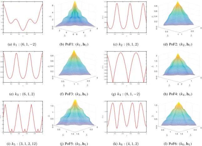
Fig. 7. Examples on different settingski: (A, B, s),i= (1,· · ·,6)in knee functionsk(XI)contribute to different PoFs. Andp= 1is set in the basic
shape functionh1, andη(x) =
√ xon all objectives. Example 1 Example 2 0 0.2 0.4 0.6 0.8 1 0 0.2 0.4 0.6 0.8 1 Contour line 1 Contour line 2 (a) (b)
Fig. 8. In (a) Example 1 and 2 plot m = (f(x) +f(y))/2 and m =
f(x)∗f(y)/2, respectively, wheref(z) = 5+10∗(z−0.5)2+cos(6πz)/2. Their corresponding contour lines are show in (b).
otherwise the PoF will be asymmetric. When there is no degeneration andk1is integrated intok(XI), the number of knees in the convex regions and concave regions is
dA
2e
m−1and(dA
2e −1)
m−1, respectively, wheremis the
number of objectives. • k2(x) k2(x) = 1 + 1 2s∗Aexp(cos(Ax Bπ+π 2)) (11)
wherex∈[0,1]. The number of knees is controlled by an integer numberA andA≥2.B controls the location of knee regions. The knee region will be skewed fors >0. When B = 1and if A is an even number, PoF will be asymmetric. An odd A will lead to a symmetrical PoF.
When no degeneration occurs and k2 is integrated into
k(XI), the number of knees in the convex regions and in the concave regions isdA
2e
m−1andbA
2c
m−1respectively,
wheremis the number of objectives.
• k3(x) k3(x) = 1 + 1 2s∗Aexp(sin(Ax Bπ+π 2)) (12)
where x ∈ [0,1]. The number of knees is controlled by an integer number A and A ≥ 2. B controls the location of knee regions. Parameter s > 0 is to skew the knee region. WhenB= 1, an odd number ofAwill lead to an asymmetrical PoF, while an even number to a symmetrical PoF. When no degeneration occurs andk3is
integrated intok(XI), the number of knees in the convex and concave regions is dA
2e
m−1 and (dA
2e −1)
m−1,
respectively, wherem is the number of objectives.
• k4(x) k4(x) = 2 + 1 2s∗A|sin(Ax B) −cos(AxB−π 4)| (13) where x ∈ [0,1]. Integer number A ≥ 2 controls the number of knees and B controls the location of knee regions. Parameters >0is used to skew the knee region. The PoF is always asymmetrical no matter whetherA is an odd or even number. When there is no degeneration and k4 is integrated into k(XI), the number of knees
in the convex and concave regions is bA+1
3 c
m−1 and
bA−1
3 c
m−1, respectively, where m is the number of
objectives. Note that the knee points in the convex regions are non-differentiable, since the minimum points in the knee function are non-differentiable. The minimums of knee function, which determine the position of the knee points, are defined by sin(AxB) =cos(AxB−π
4). • k5(x) k5(x) =2 + 1 2s∗Amin(sin(2Ax Bπ), cos(2AxBπ−π l)) (14)
where x ∈ [0,1]. Integer number A ≥ 2 controls the number of knees and B controls the location of knee regions. Parameter s > 0 is to skew the knee region. Integer numberl controls the depth of the adjacent knee regions and l ≥ 3, where a larger l will decrease the depth of a knee region. The PoF is always asymmetric no matter whether A is an odd or even number. When no degeneration occurs and k5 is integrated intok(XI), the number of knees in the convex and concave regions is (2∗A)m−1 and Am−1, respectively, wherem is the
number of objectives. Again, the knee points in the con-cave regions are not differentiable, whensin(2AxBπ) =
cos(2AxBπ−π
l), since the maximum points in the knee function are not differentiable.
• k6(x) k6(x) =2− 1 2s∗A[exp(cos(Ax Bπ)) + 0.5∗(cos(AxBπ)−0.5)4] (15)
where x ∈ [0,1]. The integer number A ≥ 2 controls the number of knees andB controls the location of knee regions. Similarly, parameter s >0 will skew the knee region. WhenB= 1, an evenAwill lead to a symmetric PoF, while an odd number to an asymmetric PoF. If no degeneration occurs andk6is integrated intok(XI), the number of knees in the convex and concave regions is
(A −1)m−1 and Am−1, respectively, where m is the
number of objectives.
C. Stretching functions η(x)
In [42], [45], the scalability of the PoF of the problems is the same on all objectives. In real-world applications, however, most problems have various scalability on different objectives. Thus, in Eq. 6, the stretching function η(x) is proposed to change the scalability of the PoF. Specifically, different combinations of elementary functions can be adopted to stretch different objectives.
These three elementary functions are adopted as follows: (1) Power function: η1(x) =Cxr; (2) Exponential function:
η2(x) =ax; (3) Logarithmic function:η3(x) =logax, where,
C,r, andaare constants.
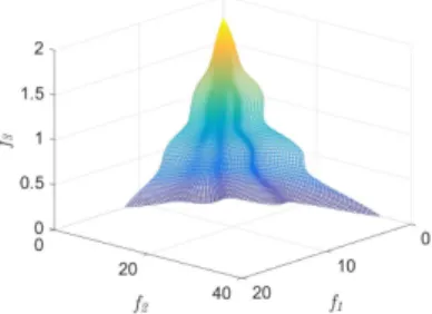
In Fig. 9, the stretching function isη(k(XI)) = 2∗k(XI) on f1, η(k(XI)) = k2(XI) on f2, η(k(XI)) = ln(k(XI)) on f3. Thus, adopting different stretching functions on the
knee functions could change the scalability of the PoF, which
Fig. 9. An example that illustrates the use of different stretching functions to change the scalability of the PoF.
creates more difficulties for an optimizer to locate the knee regions.
D. Discussions
(a)B= 1 (b)B= 3
Fig. 10. PoFs given the settings (k2,h2) and the difference between them is theBvalues in knee functionk2: (6, B,2).
1) Influence of parameterB on the PoF: Fig. 10 illustrates
the resulting PoFs given different values ofBin the basic knee functions. From the figure, we can see that when B = 3the knee regions will be shifted to the top of the PoF. Note also that
whenB >1, non-uniformity that changes the distributions of
the solutions in the objective space will be introduced.
2) Non-uniformity and degeneration the PoF: As
previ-ously discussed, non-uniformity and degeneration can be intro-duced by changing the knee function and basic shape function. For example, the following test problem constructed using the linear linkage function `1(x1, XII), landscape function
g3(XII), the basic knee function k1(XI), linear basic shape h1(XI), andη2(x) =x:
min
X :f1:m= (1 +g3(`1(x1, XII)))·η2(k1(XI))·h1(XI) (16)
(a) PoF:(6,1,−1,1) (b) PoF:(6,1,−1,1) (c) PoF:(6,1,−1,2) Fig. 11. PoFs:(A, B, s, p)withk1: (6,1,−1)but (a)k1(XI) = [k1(x1)∗ k1(x2)]/2, and p = 1in h1(XI); (b) k1(XI) = k1(x1), and p = 1 inh1(XI); (c)k1(XI) = [k1(x1)∗k1(x2)]/2, and p= 2in h1(XI).
η(k1(XI)) =
p
The Pareto front of the above test problem can be deter-mined wheng3(`1(x1, XII)) = 1holds, i.e.,`1(x1, XII) = 0 andxm+j =x11+(uii−+1li)
s
+li, whereuiandli are the upper and lower bound ofxm+ii= 0,1,· · · , n−m. Therefore, the PoF of the test problem is defined byf1:m:= (1 + 1)∗ ·k1(XI)· h1(XI).
Fig. 11(a) shows one instantiation whenA= 6,B= 1and
s=−1 in the knee function,k1(XI) = [k1(x1)∗k1(x2)]/2,
and p = 1 in h1(XI). In this case, no degeneration occurs and the PoF is not degenerate. There are nine and four knee points in the convex and concave regions, respectively.
To introduce degeneration, the knee function can be changed in such a way that it is correlated to a subset of the decision variables. For example, if we redefine k1(XI) = k1(x1),
which correlates with x1 only. As a result, the PoF becomes
degenerate onx2, refer to Fig. 11(b).
Non-uniformity of the PoF can be controlled by parameter
pin the basic shape function. For example for the above test problem, non-uniformity will be introduced when pis set to 2 in h1(XI). The resulting PoF is shown in Fig. 11(c).
3) The relationship between the knee functions and PoF:
The PoF can be formulated as follows: fi=1:m(X0) = (1 +
g(`(X0)))·η(k(X0 I))·h(X 0 I), whereX 0= min X g(`(X)). To illustrate the relationship between the knee function and PoF, Fig. 7 presents six different knee functions and their resulting PoFs. In Fig. 7(a), knee functionk1has three minima
of different peak heights, resulting in different knee regions in the PoF1. Sincek1is symmetric, PoF1 is also symmetrical as
shown in Fig. 7(b).
The two knee functions in Fig. 7(c) and Fig. 7(e), k2 and
k3, are similar. However, they result in different numbers of
knees on the PoF. If k2 is asymmetrical, PoF2 in Fig. 7(d)
is asymmetrical too. On the contrary, k3 is symmetrical and
therefore PoF3 is symmetrical as shown in Fig. 7(f).
Note that the minima ofk4 are non-differentiable, resulting
in the non-differentiable convex knee regions on PoF4, as shown in Fig. 7(g) and Fig. 7(h), respectively. In Fig. 7(i), in
k5, there are always two minimum points very close to each
other making it difficult for MOEAs to detect these two knee points. Specially, the knees in the concave regions are non-differentiable due to the non-non-differentiable maximum points in the knee function.
It is interesting to note that both knee function k6 in Fig.
7(k) and the resulting PoF6 shown in Fig. 7(l) are symmetrical but the number of knees in the concave regions on PoF6 is more than that in the convex regions.
4) Specification of knee points: As a requirement for test
functions, it is essential to specify the exact objective values of the knee points for performance evaluation. According to the way in which the benchmark problem is constructed, as described in Eq. 6, we understand that the basic knee functions are independent of each other. Consequently, a knee is defined under the condition that all basic knee functions reach the minimum or maximum.
Take the problem described in Eq. (16) as an example of how to specify the knee points, where the parameters are
(A, B, s) = (6,1,2). The first step is to identify the minima
of the knee functionk1(x)of the problem. As shown in Fig.
12(a), The knee function of problem (16) has three minima,
p1, p2, and p3, where p2 is the global minimum. According
to the superposition principle, nine minima ofk1(x1, x2)can
be calculated under the condition that bothk1(x1)andk1(x2)
reach the minimum, as shown in Fig. 12(b). Once the minima are calculated, the the knee points in the convex regions can finally be fixed by embedding them into the problem (16), as shown in Fig. 12 (c).
If problem (16) is degenerated, thenk1(x1, x2) =k1(x1).
In this case, the convex knee regions are correlated and can be determined using the minima ofk1(x1). The resulting knee
points will become lines, as shown as shown in Fig. 12(d).
5) The reference points on knee region: A common way
to obtain the representative solution set on the PoF is to minimize the landscape function and then find the well-distributed representative solutions. To be specific, we first randomly sample 10000 Pareto front points (byming(x)) and then use theK-nearest neighbor method (introduced in SPEA2 [4]) to remove the most crowded points one by one until the point size reduces to 5000. At last, they are integrated with the boundary points of the problem to construct the reference set of the PoF.
In the example (in Subsection IV-D), the linkage function isl1, and the landscape function isg3. Here, when the search
converges, ming3(l1(x1, XII)) = 1 and l1(x1, XII) = 0.0. Therefore, XII can be calculated by l1(x1, XII) = 0.0. Thus, when the solutions are randomly distributed from
(x1,· · ·, xm−1) by the normal boundary intersection [55]
or other methods, the rest components (xm,· · · , xn) can be obtained by the following Eq. 17 consequently.
In different situation, l1(x1, XII) or l2(x1, XII) can be different values. Generally, whenαis given tol1(x1, XII)or
l2(x1, XII) (in Subsection IV-D, α= 0since l1(x1, XII) =
0.0), the rest of components(xm,· · ·, xn)of variable vector can be calculated by:
l1(x1, XII) = (1+ i+ 1 s )·(xm+i−lm+i)− x1·(um+i−lm+i) =α ⇒xm+i= x1·(um+i−lm+i) +α 1 + i+1s +lm+i l2(x1, XII) = (1+cos(0.5π i+ 1 s ))·(xm+i−lm+i)− x1·(um+i−lm+i) =α ⇒xm+i= x1·(um+i−lm+i) +α 1 +cos(0.5πi+1s ) +lm+i (17) wherei= 0,1,· · · , n−m.nandmare the number of decision variables and objectives, respectively.
After a uniform set of reference points on the PoF has been preserved, we can use a clustering method to filter the reference points. Firstly, we locate the feasible knee points in terms of Subsection IV-D4. Then use the method in Subsection III-B2 and III-B3 to restrict the radius of clusters. After that, the reference points within the radius of the feasible knee points are preserved as the final reference points, where the
decision maker can also set his/her interested size of the knee regions.
E. Instantiations of Multi-objective Benchmark Problems for Knee Detection
In this section, we instantiate a set of benchmark prob-lems using the generic approach described above. Here eight landscape functions, two linkage functions, six knee functions and three basic shape functions are employed to generate the benchmark problems. Table II in the Supplementary material presents 14 instantiated benchmark problems generated using different combinations of the above functions.
In Table II in the Supplementary material, "L/NL" indicates that there is a linear or nonlinear shift of the positions of the optima. "S/NS" means that the problem is separable or non-separable. "Uni/Multi" means that the landscape function is unimodal or multimodal. "T/F" in the table basically indicates whether the related feature is true of false. For example, in the ’bias’ column, "T/F" indicates if the bias in the generated test function is present or not. No bias is present whenB= 1
and p = 1 in the knee functions and basic shape functions, respectively.
Note that when there is no bias, the symmetry of the PoF is determined by parameter Ain the knee functions. Given ı≥ 1∈Z, whenA= 2∗ı, the PoFs of PMOP1, PMOP3, PMOP6,
PMOP8-PMOP9, and PMOP12-PMOP14 are symmetrical and
A = 2∗ı+ 1 results in asymmetrical PoFs. However, A = 2∗ı+ 1will result in symmetrical PoFs on PMOP2, PMOP7 and PMOP11, but A= 2∗ıwill result in asymmetrical PoFs. It should be mentioned that the PoFs of PMOP4-PMOP5 and PMOP10 are always asymmetrical regardless whetherAis an even or odd integer.
Sinceg1andg2are unimodal functions, it shall be relatively
easy for MOEAs to converge on the resulting test problems PMOP1, PMOP2, PMOP11 and PMOP13. By contrast, the rest test problems are difficult with respect to the convergence performance since g3 − g8 are multi-modal, and PMOP4
and PMOP5 are even more difficult since g4 and g5 have
more local optima. Since PMOP10-PMOP12 and PMOP14 are embedded with two different landscape functions on different objectives, the convergence on different objectives will be different. In other words, in PMOP10-PMOP12 and PMOP14, the objectives with an odd index are specified withg3,g1,g6
andg6, respectively, and those with an even index are specified
withg7,g2,g8andg8, respectively. PMOP1, PMOP5, PMOP7,
PMOP9-PMOP11, and PMOP13 are integrated with different non-separable landscape functions.
PMOP1-PMOP12 are non-degenerate and PMOP13-PMOP14 are degenerate. It means that the knee functions k(xI) in PMOP13-PMOP14 are degenerated where
∀i ∈ {1,· · · , m−2}, signi = 1 and signm−1 = 0 in
k(xI). Thus, PMOP13 and PMOP14 have an infinite number of knee points and there are dA
2e degenerated convex knee
regions anddA
2e −1 degenerated concave knee regions.
For PMOPs without bias (p= 1 in hfunctions and B = 1 in k functions), the parameter can be set as (A, B, s) = (6,1,−2) for k1, (A, B, s) = (6,1,2) for k2−k4, k6, and
(A, B, s, l) = (3,1,2,12) for k5. All in all, by varying the
value of A we can change the symmetry of the PoFs. For PMOPs with bias, B = 2or p= 2 can be set to change the uniformity of the solutions.
V. PERFORMANCEINDICATORS
Performance indicators in multi-objective optimization are supposed to account for both accuracy and diversity of the solutions achieved by MOEAs. Popular performance indicators include generational distance (GD) [56], inverted generational distance (IGD) [57], and S-metric [58], [59], also known as hypervolume. Note that some performance indicators are dedicated to diversity [60] or spread [61] of the solutions. However, few performance indicators have been designed to evaluate the solutions obtained by MOEAs for detecting all knee points, various aspects in addition to accuracy and diversity must be taken into account. These may include the number of knee points and their accuracy in terms of the location of the detected knee points and the distribution of the solutions in the knee regions. In the following, we present three new performance indicators for evaluating the quality of the solutions in terms of their accuracy (distance to the PoF), closeness (distance to the knee point), and completeness in detecting the knee points.
Given a set of evenly distributed reference pointsQacquired in a knee region including the true knee points (K), the
knee-driven generational distance (KGD), knee-driven inverted generational distance (KIGD), and knee-driven dissimilarity (KD) for measuring the performance of a set of obtained solutionsGare defined as follows:
• Knee-driven generational distance (KGD):
KGD= 1 |G| |G| X i=1 d(νi,Q) (18)
whered(νi,Q)means the Euclidean distance between the
solution νi inG to its closest reference point inQ. The
smaller the value of KGD is, the better the set of solutions has converged to the knee region.
• Knee-driven inverted generational distance (KIGD):
KIGD= 1 |Q| |Q| X i=1 d(νi,G) (19)
where d(νi,G) means the Euclidean distance between
reference point νi in Q and the solution closest to this
reference point in G. The smaller the value of KIGD
is, the more evenly the set of solutions covers the knee region. • Knee-driven dissimilarity (KD): KD= 1 |K| |K| X i=1 d(νi,G) (20)
where d(νi,G) is the Euclidean distance between true
knee pointνifromKto its closest solution fromG, which
is designated to evaluate the completeness in identifying all knee points. Motivated by the dissimilarity measures
0 0.2 0.4 0.6 0.8 1 4 4.5 5 5.5 6 6.5 7 7.5 8 8.5 1 4 1 0.5 6 0.5 8 0 0 10 0 2 0 4 6 8 5 8 6 4 2 10 0
(a) the minima ofk1(x) (b) the minima ofk1(x1, x2). (c) the convex knees on the PoF. (d) the degenerated convex regions. Fig. 12. (a) shows the minima ofk1(x). (b) shows the minima ofk1(x1, x2). (c) shows the minima ofk1(x1, x2)acting as the convex knees on the PoF. (d) shows the degenerated minima located in the degenerated convex regions.
from multimodal optimization [62]–[64], instead of eval-uating the whole population approximating to the knee point, KD is to evaluate whether the solution set contains at least one solution close to the knee point and whether the solution set includes all the knee points. Thus, the KD indicator evaluates the solution set whether can provide a good representative solution to the decision maker so as facilitate his/her to make a choice.
KGD aims to evaluate how close the obtained solutions are to the knee regions. It mainly evaluates the search capability of the EMOAs, but also assesses their capability of identifying solutions within the knee regions because solutions outside the knee regions will degrade the performance in terms of KGD indicated by an increased KGD value. The KIGD value, by contrast, indicates how well the obtained solutions cover the knee regions, which mainly evaluates the diversity of the solutions spread over the knee regions. If the decision-maker is interested in the solutions near the knee points only rather than the knee regions, KD can assess whether there is at least one solution from the solution set is close to the knee point and whether the solution set can find all knee points. KD will become zero only when the solution set exactly covers all knee points. Thus, KD is to evaluate the capability of an algorithm to identify solutions close to the knee points.
It should be pointed out that KD is not Pareto-compliant, and it cannot differentiate two solution sets with the same proximity approximating to the same number of different knee points. Additional explanations are presented in Section II in the Supplementary material.
VI. EXPERIMENTS AND ANALYSIS
A. Experimental settings
NSGA-II [3] and RVEA [18] are chosen as the basic optimizer whilst KneeWD [37] with δ = 0.1, KneeDis [38] with4= 0.1, and KneeEMU [42] are adopted as the methods for knee identification to be embedded in NSGA-II and RVEA, respectively. Each algorithm is executed for 30 independent runs on each test instance. The population size is set as 105, 132 and 156 for 3-objective, 5-objective, and 8-objective PMOP test problems, respectively. The maximum number of generations are set to 3000 for PMOP1-PMOP3, PMOP6-PMOP9, and PMOP13, 5000 for PMOP10-PMOP12 and PMOP14, and 10000 for PMOP4 and PMOP5, respectively.
The parameters (A, B, s, p) are set as (4,1,2,1) for PMOP2-PMOP3, POMP7-PMOP8 and PMOP11-PMOP12, (2,1,2,1) for PMOP6 and PMOP9, and (4,1,-1,1) for PMOP1, and (1,1,2,1) for both PMOP5 and PMOP10 with l = 12, (6,1,-1,1) for PMOP4, (2,1,-2,1) for PMOP13 and (2,1,-(6,1,-1,1) for PMOP14. In the experiments, the distribution index is set to 20 in both the simulated binary crossover operator and polynomial mutation. The crossover probability and mutation probability are set to 1.0 and 1/n, respectively. n is the number of variables. In the comparative experiments, the Wilcoxon rank sum test (a significance level is 0.05) is adopted to analyze the results, where ‘+’, ‘−’ and ‘≈’ indicate that the result is significantly better, significantly worse and statistically similar to that obtained by NSGA-II+EMU, respectively.
B. Analysis of the Proposed Indicators
The experimental results are presented in Tables III – VII in the Supplementary material in terms of GD, KGD, IGD, KIGD, and KD values on PMOP test suite. The traditional GD and proposed KGD are adopted for evaluating the convergence performance. The results in both Table III and Table IV in the Supplementary material show that RVEA+WD, RVEA+Dis, and RVEA+EMU have significantly better GD and KGD values than NSGA-II+EMU. This is consistent with the finding that RVEA has better convergence than NSGA-II in most cases [18], especially when the number of objectives is large. The GD and KGD values also reflect the search ability of the optimizers, though they are not always consistent. This means that the preserved solutions may have good GD values but not necessarily good KGD values. For example, in Table IV in the Supplementary materials, the KGD values of NSGA-II+WD and RVEA+WD are not consistent with the GD values in Table III on the three-objective PMOP1. As shown in Fig. 2 of the Supplementary materials, the solutions in Fig. 2 (a) has large GD values than that of the solutions in Fig. 2(b). However, KGD calculates the distance from the obtained solutions to the nearest solutions in the knee regions. Thus, the KGD value of the solutions in Fig. 2(a) is smaller than that in Fig. 2(b).
From the IGD and KIGD values presented in Tables V and VI of the Supplementary material, we can see that RVEA vari-ants using different knee identification methods have achieved significantly better results than NSGA-II+EMU. Table VI of the Supplementary material compares the results obtained by RVEAs with different knee identification methods. From these
results, we can find that different knee identification methods favor different solutions and will result in different knee-driven indicator values. Similar observations can be made from the results obtained by NSGA-II using different knee identification methods. Comparing the results presented in Tables V and VI in the Supplementary material, we find that the best IGD and KIGD values are different. This can mainly be attributed to the fact that IGD favors the solutions covering the whole PoF, while KIGD favors the solutions evenly covering the knee regions.
In Table VII in the Supplementary material, indicator KD is adopted to evaluate the algorithms’ capability of converging to the knee points rather than covering the knee regions on the PoF. From these results, RVEA variants using WD, Dis and EMU have the better KD results compared with NSGA-II+EMU. Both Tables IV and VI in the Supplementary material verify that RVEAs using WD and EMU have achieved the best results. It means that KD is able to evaluate the performance of the solution set’s convergence to the knee points and the evenness in covering the knee regions. However, the KD values are also different in comparison with the KGD and KIGD values, since KD favors the solutions closer to the knee points. Fig. 3 in the Supplementary material plots the results obtained by NSGA-II+WD and RVEA+WD. The results Figs. 3 (a) and (c) (in Supplementary material) indicate that RVEA shows better convergence performance than NSGA-II. How-ever, different knee point identification methods may result in different knee-driven indicator values, because the identifica-tion methods favor different soluidentifica-tions. For example, WD [37] will choose the solutions close to the knee regions to achieve a large utility value. Thus, after selection, NSGA-II-WD may have smaller GD and KGD values than RVEA+WD, as shown Figs. 3 (b) and (d) in the Supplementary material. RVEA-WD achieves better objective values because it has better convergence performance, as shown in Figs. 3 (e) and (f) in the Supplementary materials. Thus, the search performance of the optimizers may influence the original GD and IGD values, while the knee identification method will result in different KGD and KIGD values.
The above experimental results demonstrate that KGD and KIGD are able to assess a set of solutions’ convergence to the knee points, convergence to the knee regions, and the coverage of the knee regions. If the preserved solutions are in the knee region, GD and KGD values will be consistent; otherwise, KGD will increase (degrade) since the closeness of the obtained solutions to the knee regions is accounted for by the KGD indicator. The same situation happens to IGD and KIGD. Note that KGD and KIGD not only evaluate the convergence to the knee regions and the diversity in covering the knee regions, but also take into account of the completeness in covering the knee region, i.e., whether all knee regions are covered. Finally, KD accounts for the closeness of the solutions to the knee points and completeness, i.e., whether all knee points have been identified.
C. Discussions
Five performance indicators are adopted to systematically evaluate the performance of three knee point identification
methods embedded in RVEA and NSGA-II. The experimental results show that RVEA+EMU performs the best, followed by RVEA+WD. Furthermore, the RVEA variants using different knee identification methods show overall better convergence performance than the NSGA-II variants. Results in Tables V and VI of the Supplementary material compare the diversity performance of the solution sets obtained by the compared algorithms with respect to the whole PoF and the knee regions, respectively. These results show that RVEA variants have achieved the overall best results. However, there is a large difference between the IGD and KIGD values of the solution sets obtained by the RVEAs. Moreover, the IGD and KIGD values are not always consistent. This is because IGD assesses the performance of the solution set with respect to the whole PoF while KIGD is meant for measuring the performance with respect to the knee regions only. Table VII in the Supplementary materials presents the KD values of the solutions obtained by the algorithms. These results indicate that RVEA+WD perform the best and RVEA+EMU the second best, meaning that RVEA+WD has better convergence and more obtained solutions are closer to the knee points.
In summary, the results show that RVEA using various knee identification methods show better overall convergence and diversity performance than the NSGA-II variants. However, WD and EMU are more effective in identifying knee points than Dis. Thus RVEA+WD and RVEA+EMU perform the best and the second best in locating knee solutions of the PMOP test problems.
VII. CONCLUSION
Finding preferred solutions are important in practice in solving multi- and many-objective optimization problems. Un-fortunately, littlea priori knowledge may be available for the user to specify preferences. In this case, knee points naturally become solutions of interest. However, not much work has been done to rigorously assess MOEAs’ performance in iden-tifying knee points in multi-objective, and in particular many-objective optimization problems. It is therefore of great interest to make a set of benchmark problems available for testing MOEAs’ capability in accurately and effectively identifying knee regions in high-dimensional objective spaces. For this purpose, this work proposes a generic way of constructing Pareto fronts consisting of various knee regions in terms of convexity, uniformity, symmetry, differentiability and degener-ation. To reflect other hardness in solving real-world problems, variable linkage and multi-modality are taken into account in constructing the benchmark problems. Fourteen test functions are instantiated to demonstrate the flexibility and effectiveness of the proposed method in controlling the hardness of the test problems with respect to the characteristics of the knee points as well as the fitness landscape.
In addition to the test problems, three performance in-dicators dedicated to the evaluation of MOEAs’ ability of identifying knee points are suggested, one focusing on the accuracy of the solutions, including the closeness to the Pareto front and to the knee points, the other on the effectiveness in detecting all knee regions.
Future work may include considering other naturally pre-ferred solutions such as robust optimal solutions, robust knee points, and identification of knee points for constrained prob-lems. Such considerations are of paramount importance to real-world applications and further facilitate the selection of solutions when little problem-specific preference information is available. Given the proposed benchmark problems for knee detection, it is highly desirable to develop MOEAs for efficiently and effectively detecting the knee points.
ACKNOWLEDGMENT
This work was supported in part by the Honda Research Institute Europe GmbH.
REFERENCES
[1] O. Schutze, A. Lara, and C. A. C. Coello, “On the influence of the number of objectives on the hardness of a multiobjective optimization problem,” IEEE Transactions on Evolutionary Computation, vol. 15, no. 4, pp. 444–455, 2011.
[2] K. Miettinen, “Nonlinear multiobjective optimization,” inInternational Series in Operations Research and Management Science, vol. 12. Kluwer Academic Publishers, Boston, MA, USA, 1999.
[3] K. Deb, A. Pratap, S. Agarwal, and T. Meyarivan, “A fast and elitist multiobjective genetic algorithm: NSGA-II,” IEEE Transactions on Evolutionary Computation, vol. 6, no. 2, pp. 182–197, 2002. [4] E. Ziztler, M. Laumanns, and L. Thiele, “SPEA2: Improving the
strength Pareto evolutionary algorithm for multiobjective optimization,”
Evolutionary Methods for Design, Optimization, and Control, pp. 95– 100, 2002.
[5] J. Horn, N. Nafpliotis, and D. E. Goldberg, “A niched Pareto genetic algorithm for multiobjective optimization,” in Evolutionary Compu-tation, 1994. IEEE World Congress on Computational Intelligence., Proceedings of the First IEEE Conference on. IEEE, 1994, pp. 82–87. [6] D. W. Corne, J. D. Knowles, and M. J. Oates, “The Pareto envelope-based selection algorithm for multiobjective optimization,” in Interna-tional Conference on Parallel Problem Solving from Nature. Springer, 2000, pp. 839–848.
[7] H. Ishibuchi, N. Tsukamoto, and Y. Nojima, “Evolutionary many-objective optimization,” inGenetic and Evolving Systems, 2008. GEFS 2008. 3rd International Workshop on. IEEE, 2008, pp. 47–52. [8] J. Knowles and D. Corne, “Quantifying the effects of objective space
dimension in evolutionary multiobjective optimization,” inInternational Conference on Evolutionary Multi-Criterion Optimization. Springer, 2007, pp. 757–771.
[9] S. Mostaghim and H. Schmeck, “Distance based ranking in many-objective particle swarm optimization,” inInternational Conference on Parallel Problem Solving from Nature. Springer, 2008, pp. 753–762. [10] S. Yang, M. Li, X. Liu, and J. Zheng, “A grid-based evolutionary
algorithm for many-objective optimization,”IEEE Transactions on Evo-lutionary Computation, vol. 17, no. 5, pp. 721–736, 2013.
[11] H. Sato, H. E. Aguirre, and K. Tanaka, “Controlling dominance area of solutions and its impact on the performance of MOEAs,” inInternational Conference on Evolutionary Multi-criterion Optimization. Springer, 2007, pp. 5–20.
[12] M. Laumanns, L. Thiele, K. Deb, and E. Zitzler, “Combining con-vergence and diversity in evolutionary multiobjective optimization,”
Evolutionary Computation, vol. 10, no. 3, pp. 263–282, 2002. [13] F. di Pierro, S.-T. Khu, and D. A. Savic, “An investigation on preference
order ranking scheme for multiobjective evolutionary optimization,”
IEEE Transactions on Evolutionary Computation, vol. 11, no. 1, pp. 17–45, 2007.
[14] E. Zitzler and S. Künzli, “Indicator-based selection in multiobjective search,” inInternational Conference on Parallel Problem Solving from Nature. Springer, 2004, pp. 832–842.
[15] N. Beume, B. Naujoks, and M. Emmerich, “SMS-EMOA: Multiobjec-tive selection based on dominated hypervolume,”European Journal of Operational Research, vol. 181, no. 3, pp. 1653–1669, 2007. [16] J. Bader and E. Zitzler, “HypE: An algorithm for fast hypervolume-based
many-objective optimization,”Evolutionary Computation, vol. 19, no. 1, pp. 45–76, 2011.
[17] Q. Zhang and H. Li, “MOEA/D: A multiobjective evolutionary algorithm based on decomposition,”IEEE Transactions on Evolutionary Compu-tation, vol. 11, no. 6, pp. 712–731, 2007.
[18] R. Cheng, Y. Jin, M. Olhofer, and B. Sendhoff, “A reference vector guided evolutionary algorithm for many-objective optimization,” IEEE Transactions on Evolutionary Computation, vol. 20, no. 5, pp. 773–791, 2016.
[19] K. Deb and H. Jain, “An evolutionary many-objective optimization algorithm using reference-point-based nondominated sorting approach, part i: Solving problems with box constraints.”IEEE Transactions on Evolutionary Computation, vol. 18, no. 4, pp. 577–601, 2014. [20] A. Sinha, P. Korhonen, J. Wallenius, and K. Deb, “An interactive
evolu-tionary multi-objective optimization method based on polyhedral cones,” in International Conference on Learning and Intelligent Optimization. Springer, 2010, pp. 318–332.
[21] J. Zheng, G. Yu, Q. Zhu, X. Li, and J. Zou, “On decomposition methods in interactive user-preference based optimization,”Applied Soft Computing, vol. 52, pp. 952–973, 2017.
[22] G. Yu, J. Zheng, R. Shen, and M. Li, “Decomposing the user-preference in multiobjective optimization,” Soft Computing, vol. 20, no. 10, pp. 4005–4021, 2016.
[23] R. Wang, R. C. Purshouse, and P. J. Fleming, “Preference-inspired co-evolutionary algorithms for many-objective optimization,”IEEE Trans-actions on Evolutionary Computation, vol. 17, no. 4, pp. 474–494, 2013. [24] D. K. Saxena and K. Deb, “Dimensionality reduction of objectives and constraints in multi-objective optimization problems: A system design perspective,” in Evolutionary Computation, 2008. CEC 2008.(IEEE World Congress on Computational Intelligence). IEEE Congress on. IEEE, 2008, pp. 3204–3211.
[25] M. Li, S. Yang, and X. Liu, “Shift-based density estimation for Pareto-based algorithms in many-objective optimization,” IEEE Transactions on Evolutionary Computation, vol. 18, no. 3, pp. 348–365, 2014. [26] H. Wang, L. Jiao, and X. Yao, “Two_Arch2: An improved two-archive
algorithm for many-objective optimization,”IEEE Transactions on Evo-lutionary Computation, vol. 19, no. 4, pp. 524–541, 2015.
[27] G. Yu, R. Shen, J. Zheng, M. Li, J. Zou, and Y. Liu, “Binary search based boundary elimination selection in many-objective evolutionary optimization,”Applied Soft Computing, vol. 60, pp. 689–705, 2017. [28] X. Zhang, Y. Tian, and Y. Jin, “A knee point driven evolutionary
algorithm for many-objective optimization.”IEEE Transactions on Evo-lutionary Computation, vol. 19, no. 6, pp. 761–776, 2015.
[29] S. F. Adra, I. Griffin, and P. J. Fleming, “A comparative study of progressive preference articulation techniques for multiobjective opti-misation,” inInternational Conference on Evolutionary Multi-Criterion Optimization. Springer, 2007, pp. 908–921.
[30] A. Mohammadi, M. N. Omidvar, and X. Li, “Reference point based multi-objective optimization through decomposition,” in Evolutionary Computation (CEC), 2012 IEEE Congress on. IEEE, 2012, pp. 1–8. [31] C. C. Coello, “Handling preferences in evolutionary multiobjective
op-timization: A survey,” inEvolutionary Computation, 2000. Proceedings of the 2000 Congress on, vol. 1. IEEE, 2000, pp. 30–37.
[32] H. Wang, M. Olhofer, and Y. Jin, “A mini-review on preference modeling and articulation in multi-objective optimization: current status and challenges,”Complex & Intelligent Systems, vol. 3, no. 4, pp. 233– 245, 2017.
[33] J. Clímaco and J. Craveirinha, “Multiple criteria decision analysis–state of the art surveys,” International Series in Operations Research and Management Science, pp. 899–951, 2005.
[34] I. Das, “On characterizing the knee of the Pareto curve based on normal-boundary intersection,” Structural Optimization, vol. 18, no. 2-3, pp. 107–115, 1999.
[35] S. Bechikh, L. B. Said, and K. Ghédira, “Searching for knee regions of the Pareto front using mobile reference points,”Soft Computing, vol. 15, no. 9, pp. 1807–1823, 2011.
[36] K. S. Bhattacharjee, H. K. Singh, and T. Ray, “A study on performance metrics to identify solutions of interest from a trade-off set,” in Aus-tralasian Conference on Artificial Life and Computational Intelligence. Springer, 2016, pp. 66–77.
[37] L. Rachmawati and D. Srinivasan, “Multiobjective evolutionary algo-rithm with controllable focus on the knees of the Pareto front,” IEEE Transactions on Evolutionary Computation, vol. 13, no. 4, pp. 810–824, 2009.
[38] O. Schütze, M. Laumanns, and C. Coello Coello, “Approximating the knee of an MOP with stochastic search algorithms,”Parallel Problem Solving from Nature–PPSN X, pp. 795–804, 2008.