Integrating decomposition methods with user preferences for solving many-objective optimization problems
A thesis submitted in fulfilment of the requirements for the degree of Doctor of Philosophy
Asad Mohammadi
Master of Computer Science
School of Science
College of Science, Engineering and Health RMIT University
I certify that except where due acknowledgement has been made, this work is that of the author alone; the work has not been submitted previously, in whole or in part, to qualify for any other academic award; the content of the thesis is the result of work which has been carried out since the official commencement date of the approved research program; and, any editorial work, paid or unpaid, carried out by a third party is acknowledged. I acknowl-edge the support I have received for my research through the provision of an Australian Government Research Training Program Scholarship.
Asad Mohammadi
School of Science (Computer Science and Software Engineering) RMIT University
Acknowledgments
The compilation of this thesis would not have been possible without the help and support of the following.
• I would like to thank my supervisors, Professor Xiaodong Li and Professor Kalyanmoy Deb for their help and support during my candidature.
• I would like to express my heartfelt thanks to Dr. Nabi Omidvar for his valuable inputs and guidance during this research.
• I want to thank ECML members especially, Assoc. Professor Vic Ciesielski, Dr.Yi Mei, Dr. William Raffe, Mr Sven Schellenberg and Mr. Borhan Kazimipour for their grateful comments and feedbacks.
• Many thanks to Shane Talia and Greg Rowe for proof-reading and editing this thesis.
• Last but not least I would like to sincerely thank my family and friends for the emotional support and continual during the difficult times that I experienced in the last two years of my PhD. I wholeheartedly appreciate everything they have done for me.
I would also like to thank the Australian government and RMIT University (School of Science) for funding this research, without which I could not have completed the work.
Credits
Portions of the material in this thesis have previously appeared in the following publications:
• Mohammadi, A., Omidvar, M., Li, X., Deb, K. and X. Yao (2017), “Feedback Mecha-nism for Decomposition-Based Evolutionary Many-Objective Optimization”.IEEE Trans-actions on cybernetics. (under review)
• Mohammadi, A., Omidvar, M., Li, X. and Deb, K. (2015), “Sensitivity Analysis of Penalty-based Boundary Intersection on Aggregation-based EMO Algorithms”, in Pro-ceedings of Congress of Evolutionary Computation (CEC 2015), IEEE, 2015, p.2891-2898.
• Mohammadi, A., Omidvar, M., Li, X. and Deb, K. (2014), “Integrating User Prefer-ences and Decomposition methods for Many-objective Optimization”, in Proceedings of Congress of Evolutionary Computation (CEC 2014), IEEE, 2014, p.421 - 428.
• Mohammadi, A., Omidvar, M. and Li, X. (2013), “A New Performance Metric for User-preference Based Multi-objective Evolutionary Algorithms”, inProceedings of Congress of Evolutionary Computation (CEC 2013), IEEE,2013, p.2825 - 2832.
• Mohammadi, A., Omidvar, M. and Li, X. (2012), “Reference Point Based Multi-objective Optimization Through Decomposition”, in Proceedings of Congress of Evo-lutionary Computation (CEC 2012), IEEE, 2012, p.1150 - 1157.
Abstract 2 1 Introduction 3 1.1 Motivation . . . 3 1.2 Research Objectives . . . 7 1.3 Methodology . . . 8 1.4 Contributions . . . 8
1.5 Overview of the Study and Organization . . . 9
2 Literature Review 11 2.1 Multi-objective Optimization . . . 12
2.1.1 Dominance Relation . . . 13
2.1.2 Many-objective Optimization . . . 13
2.2 Classical Methods to Solve Multi-objective Problems . . . 14
2.2.1 The Weighted-Sum Approach . . . 14
2.2.2 The Tchebycheff Approach . . . 15
2.2.3 The Penalty-Based Boundary Intersection Approach . . . 16
2.3 Metaheuristics Algorithms . . . 17
2.3.1 Evolutionary Algorithms (EAs) . . . 17
2.3.2 Differential Evolution (DE) . . . 19
2.4 Evolutionary Multi-objective Optimization (EMO) Algorithms . . . 20
2.4.1 Non-elitist Approaches . . . 20
2.4.2 Elitist Approaches . . . 22
2.4.3 Decomposition-Based EMO Algorithms . . . 23
2.5.1 a priori Methods . . . 27
2.5.2 a posteriori Methods . . . 30
2.5.3 Interactive Methods . . . 31
2.6 Performance Metrics in EMO . . . 33
2.6.1 Cardinality-Based Metrics . . . 33
2.6.1.1 Set Convergence Metric . . . 34
2.6.1.2 Convergence Difference of Two Sets . . . 34
2.6.2 Distance-Based Metrics . . . 35
2.6.3 Volume-Based Metrics . . . 36
2.6.4 User-Preference Performance Metrics in EMO . . . 36
2.7 Summary . . . 38
3 Applying User Preferences on Decomposition Methods 39 3.1 Introduction . . . 39 3.2 R-MEAD . . . 41 3.3 Experimental Settings . . . 43 3.3.1 Parameter Settings . . . 43 3.4 Analysis of Results . . . 44 3.4.1 Benchmark Results . . . 44
3.4.2 Comparison between Weighted-Sum and Tchebycheff . . . 44
3.4.3 Faster Convergence to the Pareto-optimal front . . . 48
3.5 Chapter Summary . . . 49
4 A User-preference Based Method for Solving Many Objective Problems 51 4.1 Introduction . . . 51
4.2 Proposed approach (R-MEAD2) . . . 52
4.2.1 The R-MEAD2 Algorithm . . . 53
4.3 Experimental Results and Analysis . . . 56
4.3.1 RNG vs GLP . . . 56
4.3.2 Parameter Settings and Performance Metrics . . . 57
4.3.3 Weight Vector Convergence . . . 58
4.3.4 Numerical Results . . . 58
5 Sensitivity Analysis of the Penalty Parameter in PBI 63
5.1 Introduction . . . 63
5.2 Experimental Design . . . 64
5.2.1 Parameter Settings . . . 64
5.2.2 Performance Metrics . . . 64
5.3 Analysis and Discussion . . . 65
5.4 Chapter Summary . . . 71
6 Feedback Mechanism for Decomposition-Based Evolutionary Many-Objective Optimization 73 6.1 Introduction . . . 73
6.2 Proposed Approach UR-MEAD2 . . . 74
6.2.1 Overlapping Hypervolume . . . 75
6.2.2 Potential Energy . . . 77
6.2.3 Potential Energy with Direction Vector . . . 79
6.2.4 The UR-MEAD2 Algorithm . . . 80
6.2.4.1 OHV . . . 82
6.2.4.2 PE . . . 82
6.2.4.3 PEV . . . 84
6.3 Experimental Results and Analysis . . . 84
6.3.1 Parameter Settings and Performance Metrics . . . 84
6.3.2 The Effect of Using a Feedback Mechanism . . . 85
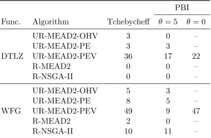
6.3.3 The Effect of Decomposition Methods on PEV . . . 86
6.3.4 Behavior of UR-MEAD2 without reference point . . . 92
6.3.5 Sensitivity analysis of UR-MEAD2 to weight vector update frequency 92 6.4 Chapter Summary . . . 95
7 A Novel Performance Metric for User-preference based Algorithms 98 7.1 Introduction . . . 98
7.2 Proposed Metric (UPCF) . . . 99
7.3 Simulation Results . . . 101
7.3.1 Two-Objective Test Problems . . . 106
7.3.2 Three-Objective Test Problems . . . 106
7.3.4 Result Analysis . . . 110 7.4 Chapter Summary . . . 114
8 Conclusion 116
8.1 Research Objectives Revisited . . . 117 8.2 Future Research . . . 121
Appendices 123
A Multi-objective Optimization Test Problems 125
B IGD,GD and L2 results on DTLZ1-DTLZ6 test problems using PBI
de-composition with different penalty parameters 128
C Hypervolume and IGD results for UR-MEAD2 Method 135
2.1 An example of a multi-objective optimization problem . . . 12
2.2 Illustration of the weighted-sum approach on a convex Pareto-optimal front . 15 2.3 Illustration of the Tchebycheff method. . . 16
2.4 Illustration of the PBI method. . . 17
2.5 An example to depict the deficiency of the metric proposed in [Wickramasinghe et al., 2010]. . . 37
3.1 Effect of updating the weight vectors in moving the solutions closer to the desired region. . . 40
3.2 ZDT1-ZDT4, ZDT6 benchmark functions using Tchebycheff . . . 45
3.3 ZDT1-ZDT4 and ZDT6 benchmark functions using weighted-sum . . . 46
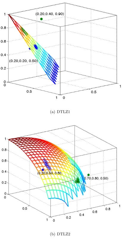
3.4 DTLZ1 and DTLZ2 benchmark functions using Tchebycheff . . . 47
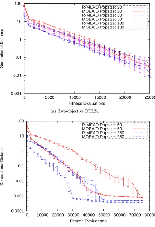
3.5 Convergence of GD for R-MEAD and MOEA/D on DTLZ1 . . . 50
4.1 Illustration how weight vectors are updated in RMEAD-2 . . . 54
4.2 Weight vector convergence behavior . . . 59
5.1 Relationship betweenθ and number of objectives . . . 72
6.1 Illustration of the overlapping Hypervolume method. . . 76
6.2 Illustration of the Potential Energy (PE) method. . . 78
6.3 Illustration of how the weight vectors are updated when PE and OHV are used in UR-MEAD2 . . . 81
6.4 Illustration of updating weight vectors based on direction vector and closeness to the reference point in UR-MEAD2 (PEV) . . . 83
6.6 Objective value plots on 10-objective DTLZ2 and WFG7 . . . 94
7.1 Composite front which is used to define a preferred region . . . 100
7.2 Results on ZDT1, ZDT2, ZDT4 and ZDT6 function . . . 108
4.1 R-MEAD pop-size for different objectives (H = 10). . . 52
4.2 The average CD2 value of 25 independent runs for GLP and RNG . . . 56
4.3 IGD values on DTLZ1-DTLZ6 test problems . . . 62
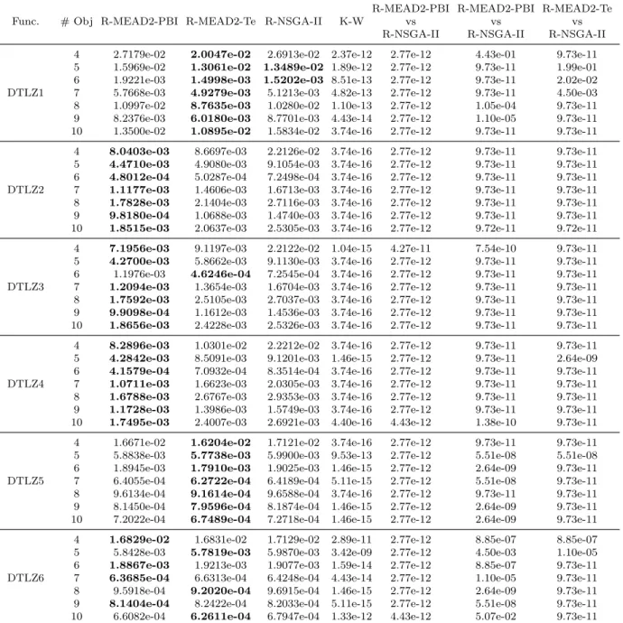
4.4 R-NSGA-II against R-MEAD2-Te and R-MEAD2-PBI . . . 62
II Spearman correlation coefficients with respect to different metrics . . . 67
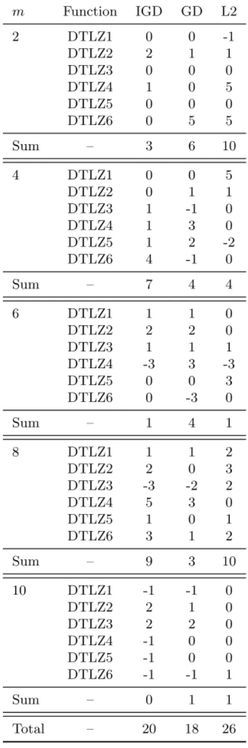
III Success frequency of various θ values. Using IGD,GD and L2 metrics on MOEA/D and R-MEAD2 . . . 67
IV Differences between MOEA/D and R-MEAD2 of best performing θ values . . 69
V Differences between indices of the best performing θ values of IGD and GD, as well as IGD and L2-discrepancy. . . 69
6.1 Number of times each algorithm has the best performance as compared to other algorithms(HV results). . . 90
6.2 Number of times each algorithm has the best performance as compared to other algorithms.(IGD results) . . . 91
6.3 Number of times UR-MEAD2-PEV has the best performance in different de-composition methods(HV Values) . . . 92
6.4 Number of times UR-MEAD2-PEV has the best performance in different de-composition methods(IGD Values) . . . 92
6.5 HV values of UR-MEAD2 with TE using different frequency parameters of updating weight vectors. . . 97
7.1 Nadir points for two and three-objective test problems . . . 101
7.2 Nadir points for 3,5 and 7 objective test problems . . . 102
7.4 Results on the three-objective test problems. . . 105
7.5 Results on the 5-objective test problems . . . 111
7.6 Results on the 7-objective test problems . . . 112
7.7 Results on the 10-objective test problems. . . 113
7.8 Consistency of each measure with IGD-OF for 2 and 3 objective problems . . 114
7.9 Consistency of each measure with IGD-OF for 5,7 and 10-objective problems 115 A.1 Features of ZDT Test Problems . . . 126
A.2 Features of DTLZ Test Problems . . . 126
A.3 Features of WFG Test Problems . . . 127
B.1 IGD,GD andL2 values on DTLZ1 test problem . . . 129
B.2 IGD,GD andL2 values on DTLZ2 test problem . . . 130
B.3 IGD,GD andL2 values on DTLZ3 test problem . . . 131
B.4 IGD,GD andL2 values on DTLZ4 test problem . . . 132
B.5 IGD,GD andL2 values on DTLZ5 test problem . . . 133
B.6 IGD,GD andL2 values on DTLZ6 test problem . . . 134
C.1 HV values for PBI decomposition method on DTLZ1-DTLZ6 test problems . 136 C.2 HV values for TE decomposition method on DTLZ1-DTLZ6 test problems . . 137
C.3 HV values for PBI decomposition method on WFG1-WFG9 test problems . . 138
C.3 HV values for PBI decomposition method on WFG1-WFG9 test problems . . 139
C.4 HV values for TE decomposition method on WFG1-WFG9 test problems. . . 140
C.4 HV values for TE decomposition method on WFG1-WFG9 test problems. . . 141
C.5 HV values for TE and PBI (PEV variant) on DTLZ test problems . . . 142
C.6 HV values for TE and PBI (PEV variant) on WFG test problems. . . 143
C.6 HV values for TE and PBI (PEV variant) on WFG test problems. . . 144
C.7 IGD values for PBI decomposition method on DTLZ1-DTLZ6 test problems . 145 C.8 IGD values for TE decomposition method on DTLZ1-DTLZ6 test problems. . 146
C.9 IGD values for PBI decomposition method on WFG1-WFG9 test problems. . 147
C.10 IGD values for TE decomposition method on WFG1-WFG9 test problems. . 149
C.11 IGD values for TE and PBI (PEV variant) on WFG test problems. . . 151
This research aims to investigate methods to solve many-objective (a multi-objective prob-lem with three or more objectives) optimization probprob-lems. To achieve this, we propose an algorithm combining user-preference and decomposition approaches. The main reasons that decomposition-based evolutionary multi-objective optimization (EMO) methods are em-ployed in this research are: firstly, they suffer less from the selection pressure issue in com-parison to dominance ranking as they rely on decomposition methods such as Weighted-sum, Tchebycheff and Penalty-based Boundary Intersection (PBI) to convert a multi-objective problem into a set of single-objective problems. Secondly, decomposition approaches employ a set of weight vectors which give us a reasonable control of solutions in the objective space. As user-preference approaches alleviate the scalability issue of many-objective problems, they are adopted in this research. User-preference methods can potentially save a considerable amount of computational resources by searching on more desired regions rather than the entire Pareto-optimal front. In this research, user-preference is defined in the form of one or more reference points or directions. The proposed algorithm outperforms R-NSGA-II which is one of popular dominance-based approaches on many-objective optimization problems.
Finding a diverse set of solutions is another major challenge for EMOs. The issue of so-lution diversity is of greater importance when dealing with many-objective problems. In this thesis, we propose an algorithm using a mechanism to update the weight vectors according to feedback that quantifies the uniformity of the solutions in the objective space. Two existing metrics and a newly developed metric are adopted as feedback mechanisms. These metrics allow us to assess the contribution of each solution towards improving the overall uniformity of the solution set in the objective space, and to use this information to update the weight vectors adaptively so that the overall uniformity is maintained. The overarching is to iden-tify sparse areas in the objective space, and move the solutions from the denser to sparse areas. The newly developed metric uses the idea of electrostatic equilibrium to calculate the
explicit means of controlling the uniformity of solutions in the objective space.
Since existing metrics are neither sufficiently accurate nor scalable to measure the per-formance of user-preference based EMO algorithms, we develop a new perper-formance metric to fill this gap. The proposed metric uses a composite front as a substitute for the Pareto-optimal front then a preferred region is defined on the composite front. Performances of the new metric are compared against a baseline which relies on knowledge of the Pareto-optimal front. One of the key advantages of the proposed metric is that it does not depend on prior knowledge of the Pareto-optimal front of a particular problem, which is most likely the case in real-world situations.
Introduction
1.1 MotivationThe term optimization refers to finding one or more optimal solutions which correspond to the maximum or minimum values of one or more objectives [Schwefel, 1993; Ben-Tal and Nemirovski, 2002; Gill et al., 1981]. Optimization techniques have been applied to many problems such as engineering design and manufacturing industries [Coello et al., 1999]. There are different types of optimization problems. When there is only one objective, it is called single-objective optimization. The main goal of a single-objective optimization method is to find the best solution which corresponds to the maximum or minimum value of the objective function. When optimization involves more than one objective function and these objectives tend to conflict with each other, it is called multi-objective optimization. Multi-objective optimization problems are very important to both scientists and engineers as most real-world problems could be considered as multi-objective [Deb, 2001; Coello et al., 2006]. Some applications that use multi-objective optimization techniques are job scheduling [Xia and Wu, 2005], manufacturing the shape of turbine blades and aeroplane wings [Hughes, 2007; Takagi, 2001]. There are different methods used to solve optimization problems including classical methods [Miettinen, 1999; Laumanns et al., 2006; Miettinen, 1999; Benson, 1978; Keeney and Raiffa, 1993]. However, these methods are not effective to solve linear, non-convex and multi-objective optimization problems [Deb, 2001; Schwefel, 1993]. Evolutionary algorithms (EAs) [Back, 1996] are one of the alternatives to classical methods. EAs are based on Darwin's theory of evolution where the selection pressure allows fitter individuals to survive to the next generation. EAs evolve a population of potential solutions in successive iterations of the algorithm to find a set of candidate solutions.
In recent years, there has been a growing interest in the area of many-objective optimiza-tion [Hughes, 2005a]. That is a multi-objective optimizaoptimiza-tion problem having three or more objectives, which is the main focus of this research. However, the performance of evolutionary multi-objective approaches degrades rapidly as the number of objectives increases [Ishibuchi et al., 2008a;b]. There are several challenges that Evolutionary multi-objective Optimization (EMO) algorithms are faced with when they are dealing with many-objective problems [Deb et al., 2006]. Firstly, visualizing the Pareto-front when there are more than three objectives is very difficult. It is challenging for the decision maker (DM) to get a visual sense of the solutions accurately and to be able to select a preference. Another challenge is related to the number of solutions required to approximate the Pareto-optimal front. In other words, the number of solutions increases exponentially with respect to the number of objectives. Finally, in the case of dominance-based approaches such as NSGA-II [Deb et al., 2002], SPEA [Zitzler and Thiele, 1999] and MOGA [Fonseca and Fleming, 1993] when the number of objectives increases, most of the solutions, even in the initial randomly generated population, are non-dominated to each other. This suggests that none of the objective functions can be improved in value without degrading some of the other objective values. As a result, there will not be enough selection pressure to propel the solutions towards the Pareto-optimal front [Ishibuchi et al., 2008b;a]. To overcome the scalability issue of Pareto dominance EMO approaches, we propose to investigate the following two strategies:
1. Replacing dominance ranking by using decomposition techniques.
2. Confining the search space and focus on specific parts of the Pareto-optimal front instead of finding the entire Pareto-optimal front, which helps to reduce the computa-tional cost.
Decomposition strategies, which are borrowed from multi-criteria decision making [Hughes, 2005b], can alleviate the selection pressure problem imposed on dominance-based evolution-ary algorithms. They convert a multi-objective problem into a set of single objective prob-lems. In other words, since decomposition methods do not use dominance comparisons, they are scalable to a greater number of objectives. Decomposition methods use different scalariz-ing functions that assign a set of weights to the objective functions. When these scalarizscalariz-ing functions are used in conjunction with population-based metaheuristics, they can solve the resultant single objective problems with various weight values, resulting in obtaining so-lutions on different parts of the Pareto front. This makes the decomposition-based EMO algorithms less sensitive to the selection pressure issue. MOEA/D [Zhang and Li, 2007]
and MOGLS [Ishibuchi and Murata, 1998] are two popular EMO algorithms that eliminate dominance ranking by employing scalarizing functions. One of the main reasons that we use decomposition methods in this research is that they provide an explicit means of controlling where a population converges by changing the weight vectors. This can also be used to control the distribution of solutions directly.
Adopting user-preference based approaches, e.g. a reference point, is another promising way of alleviating the scalability issue of EMO algorithms. Using a reference point allows us to save considerable computational resources by focusing the search on more desirable regions on the Pareto-optimal front instead of searching the entire Pareto-optimal front. In this approach the user may have one or more existing solutions that were obtained through various means and can be passed to the algorithm as a reference point(or points). For instance, in a car-buying decision-making multi-objective problem, there are two conflicting objectives: cost and comfort. A car with a price of $30,000 and a comfort level of 60% can be passed to the algorithm as a reference point. There are various types of user-preference methods includinga priori (where a user defines his/her preferences before the search process),interactive (where a user defines his/her preferences during the search process), and a posteriori (where a user defines his/her preferences after the search process) decision making. Some of the popular user-preference based EMO algorithms are R-NSGA-II [Deb et al., 2006] which uses reference points to incorporate the user preferences, RD-NSGA-II [Deb and Kumar, 2007b] which uses reference direction for the same purpose, LBS-NSGA-II [Deb and Kumar, 2007a] which uses a light beam approach to incorporate user preferences and PICEA [Wang et al., 2013] which is an example ofa posteriori decision making. Since applying scalarization techniques to some extent alleviates the selection pressure issue of dominance-based approaches, and utilizing user-preference information reduces computational cost, this research combines both methods. In chapters 3 and 4, we develop user-preference decomposition based algorithms to solve many-objective optimization problems. One of the main advantages of this combination is that utilizing weight vectors of decomposition methods helps in handling user-preferences by guiding solutions towards the preferred region.
MOEA/D, which is the basis of our proposed approaches in this thesis, has been tested with two scalarizing functions: Tchebycheff and PBI. The Tchebycheff method works well on both convex and non-convex Pareto-optimal fronts, but does not result in a very uniform set of solutions on the Pareto-optimal front [Zhang and Li, 2007]. Penalty-based Boundary Intersection (PBI) is a variation of Normal Boundary Intersection (NBI) [Das and Dennis, 1998] that uses a simple penalty method to eliminate the need for direct handling of NBI’s
equality constraint. PBI generally produces more uniform solutions than Tchebycheff, but its convergence can be affected by its penalty parameter (θ) which has not been well-studied. As a result, chapter 5 of this thesis presents a sensitivity analysis of the PBI penalty parameter. Finding uniformly distributed solutions in the objective space is a major challenge in EMO. Two main difficulties of finding a uniform set of solutions on the Pareto front are as follows:
1. An accurate metric is needed to measure the uniformity of solutions in the objective space.
2. Most of the existing metrics measure the uniformity of the entire solution set, but they are unable to rank the individuals in terms of their contributions to the overall uniformity. In other words, most of the uniformity metrics face a credit assignment problem.
Several metrics [Deb et al., 2002; Pettie and Ramachandran, 2002; Silverman, 1986; Huang et al., 2005] have been proposed to address the uniformity issue. However, most of these metrics are not scalable to many-objective optimization problems [Purshouse and Fleming, 2007; Hughes, 2005b]. Maintaining the diversity of solutions becomes even more difficult in many-objective problems since the size of the search space grows exponentially. Therefore, the accuracy of current metrics degrades severely in high dimensional spaces.
As previously mentioned, one of the main features of decomposition methods is controlling the distribution of solutions by adjusting weight vectors. The following question arises when dealing with decomposition methods: How to generate a set of weight vectors for a given aggregation function in order to ensure a desired level of diversity among the solutions? Some approaches [Tan et al., 2013; Qi et al., 2014; Ma et al., 2014] replace the weight vector initialization method in MOEA/D (Simplex-lattice design) with a good lattice point (GLP) and other complex weight vector initialization methods to generate uniform solutions. However, most of those algorithms are not efficient in finding uniform solutions as they either use sophisticated methods which can be computationally expensive or they rely on the information of the Pareto-optimal front to generate a set of well distributed weight vectors. Since the relationship between the weight space and the objective space is not always linear, generating a uniform set of solutions from a uniform set of weight vectors is not always possible. Relying on Pareto-optimal front information to engineer weight vectors to obtain a uniform set of solutions is also not viable since this information is not always available. As a result, there is a need for a mechanism during the course of optimization
to maintain this unique relationship between the weight vectors and solutions in objective space. In other words, weight vectors should be dynamically updated during the course of optimization with the aim of generating a uniform set of solutions in the objective space. To achieve this, in chapter 6 of this thesis a feedback mechanism is proposed. Some existing metrics [Van Moffaert et al., 2014; Ong et al., 2012] have been used to measure the uniformity of solutions and a new uniformity metric is also proposed.
Finally, since very few metrics exist [Veldhuizen and Lamont, 2000; Zitzler et al., 2003; Veldhuizen, 1999a] to measure the performance of user-preference approaches accurately, in chapter 7 we develop a metric to compare the performance of user preference-based algorithms fairly. The main novelties of this metric compared to existing metrics are: 1) It measures both convergence and diversity of the solutions in the preferred regions independent of any parameters such as nadir points; and 2) it is scalable when the number of objectives increases since it is independent of the knowledge of the Pareto-optimal front.
1.2 Research Objectives
This research will focus on addressing the following objectives:
1. To develop a novel method by combining the decomposition and user preference meth-ods for better handling many objective optimization problems
2. To evaluate the effect of penalty parameters in PBI on the performance of user-preference and non-user-user-preference EMO algorithms
3. To design a new technique to improve the uniformity of solutions in the preferred region particularly when the shape of the Pareto-optimal front is complex or highly non-linear. To investigate a mechanism which can find a diverse set of solutions without the knowledge of the Pareto-optimal front
4. To define a new metric to evaluate the performance of different user-preference based algorithms
The next section presents techniques which are developed to address these research ques-tions.
1.3 Methodology
Decomposition and user-preference are two main techniques adopted in this research to ad-dress the objectives stated above. In this research, we make use of user preference information through the form of reference points, which can be one of the existing solutions in the objec-tive space. We use three different decomposition methods: Weighted-Sum [Miettinen, 1999], Tchebycheff [Miettinen, 1999], Boundary Intersection [Das and Dennis, 1998], and Penalty-based Boundary Intersection [Zhang and Li, 2007]. A set of multi-objective optimization benchmark functions with different Pareto-optimal shapes are used to evaluate the perfor-mance of the proposed algorithms. To measure the quality of solutions generated by the proposed approaches, both convergence and diversity aspects have been measured simulta-neously and separately. Since existing metrics used in the field are not designed specifically to measure the quality of solutions in the preferred regions, the performance metrics take user-preference information into account. To assess the capability of the proposed methods in terms of finding optimal solutions, visualization tools have also been used. To determine whether the results are significantly different, a non-parametric statistical test is run on the results. In order to rank the algorithms, we used the Mann-Whitney-Wilcoxon (MWW) test with a Bonferroni correction only when the null hypothesis of Kruskal-Wallis was rejected under a 95% confidence interval.
1.4 Contributions
This thesis makes novel contributions to the field of EMO, particularly to many-objective optimization. The core of these contributions is about combining decomposition methods with user-preference models for solving many-objective optimization problems. In particular the key contributions are as follows:
1. The development of scalable decomposition and user-preference based multi-objective algorithms which can be applied to many-objective optimization problems. The pro-posed algorithm is less susceptible to the selection pressure, focused in the preferred region and converges on the Pareto-optimal front more rapidly.
2. The development of a more effective mechanism updating weight vectors and decoupling the population size and number of objectives. This makes the proposed approach more effective in higher numbers of objectives.
3. The development of a sensitivity analysis of penalty parameter in PBI. In order to do so, the effect of penalty parameter has been studied according to (a) the problems with and without user-preference information; (b) the convergence and uniformity of the solutions separately and simultaneously; and (c) the performance of the algorithm as the number of objectives increases.
4. The development of a mechanism to maintain the uniformity of solutions in user-preference based approaches by providing feedback from the behavior of solutions in the objective space to weight vectors. Dynamically adapting the weight vectors according to the solutions in the objective space during the course of optimization is the main novelty of this approach. To achieve this, a new uniformity metric is proposed, and the results are compared with those using existing metrics.
5. The development of a metric to measure the performance of user-preference based EMO algorithms so that we can compare preference-based EMO algorithms more fairly. The main idea has been borrowed from cardinality-based metrics. A composite front has been formed to replace the Pareto-optimal front and the preferred regions have been defined on it.
1.5 Overview of the Study and Organization
Chapter 2 first provides the basic definitions for multi-objective optimization with example problems. Next, we present a review of classical methods and evolutionary algorithms to solve multi-objective optimization problems. The literature review of decomposition and user-preference based EMO approaches are also presented. Finally, the performance metrics which are used in this thesis are described and reviewed.
In chapter 3, we propose a user-preference based evolutionary algorithm that relies on decomposition strategies to convert a multi-objective problem into a set of single-objective problems. The proposed approach is called R-MEAD. The use of a reference point allows the algorithm to focus the search on more preferred regions, which can potentially save a con-siderable amount of computational resources. Combining decomposition strategies with ref-erence point approaches paves the way for the more effective optimization of many-objective problems.
In chapter 4, we propose a user-preference based evolutionary multi-objective algorithm that uses decomposition methods for solving many-objective problems. The newly proposed
algorithm, R-MEAD2, improves the scalability of its previous version (R-MEAD) by adopt-ing a Simplex-lattice design method for generatadopt-ing weight vectors. This makes the population size independent from the dimension size of the objective space. R-MEAD2 uses a uniform random number generator (RNG) to remove the coupling between dimension and the pop-ulation size. It should be noted that a uniform set of weight vectors does not necessarily map to a uniform set of solutions in the objective space, especially on highly non-linear and complex Pareto-optimal fronts. This requires a feedback mechanism to adjust the weights in order to obtain a set of uniform solutions, which is the main topic of chapter 6.
As indicated previously, MOEA/D relies on decomposition methods such as weighted-sum, Tchebycheff and Penalty-based Boundary Intersection (PBI), to convert a multi-objective problem into a set of single-objective problems. It has been argued that PBI can generate a more uniform set of solutions than other decomposition methods. However, the main draw-back of PBI is that it has a penalty parameter (θ) which needs to be specified by the user. This penalty parameter can affect the convergence as well as the uniformity of solutions. Chapter 5 provides a comprehensive analysis of PBI’s penalty parameter and its effect on a user-preference algorithm (R-MEAD2), and a non-user-preference algorithm (MOEA/D) has been conducted. Also in this chapter, the effect of θon convergence, uniformity and the combination of convergence and uniformity have been analyzed.
Since generating a uniform set of solutions turns out to be a challenging task for multi-objective optimization problems, chapter 6 provides a strategy to tackle this. A feedback mechanism is developed to assess the uniformity of solutions in the objective space dur-ing the course of optimization. These feedback values are then used to dynamically adapt weight vectors for better solution uniformity in the objective space. The proposed method (UR-MEAD2) can adopt any uniformity metrics as a feedback mechanism. More specifi-cally, adopted metrics are used to rank individuals in terms of their contributions towards improving the overall solution uniformity.
In chapter 7, we propose a metric for evaluating the performance of user-preference based EMO algorithms. It defines a preferred region based on the location of a user-supplied reference point. This metric uses a composite front which is a type of reference set and is used as a replacement for the Pareto-optimal front. This composite front is constructed by extracting the non-dominated solutions from the merged solution sets of all algorithms that are to be compared. A preferred region is then defined on the composite front based on the location of a reference point. Once the preferred region is defined, existing evolutionary multi-objective performance metrics can be applied with respect to that region.
Literature Review
Since the late 1990s, the number of applications of multi-objective evolutionary algorithms (MOEAs) has grown considerably. The main reason behind this increase is the success of MOEAs in solving real-world problems. In recent years, many-objective optimization has become more popular. However, only a limited number of many-objective real-world applications exists since there is no efficient and effective technique to handle many-objective optimization problems. In this thesis, we have developed some user-preference Evolutionary Multi-objective Optimization algorithms (EMOs) which are able to solve many-objective optimization problems effectively. Before we get into the details of the proposed algorithms it is important to describe the background materials and literature related to the research presented in this thesis. First, in Section 2.1, some key concepts involving multi-objective and many-objective optimization are introduced. In Section 2.2, classical methods to solve multi-objective optimization problems are presented with their shortcomings identified to justify the use of Evolutionary Algorithms (EAs). Concepts of EAs with examples are described briefly in Section 2.3.1. Next, in Section 2.4, we present how EMOs are developed. Some issues that EMO algorithms are facing to solve many-objective optimization problems are also illustrated. Section 2.5 presents techniques found in the literature in tackling these issues. In this section, popular user-preference EMO algorithms are illustrated in detail. Finally in Section 2.6, existing performance metrics for user-preference and non-user-preference EMO algorithms in the literature are described.
Figure 2.1: An example of a multi-objective optimization problem 2.1 Multi-objective Optimization
An optimization problem involving one objective is called a single-objective optimization. The main goal of a single-objective optimization method is to find the best solution, which corresponds to the maximum or minimum value of an objective function. When an opti-mization involves more than one objective function and these objectives tend to conflict with each other, it is called multi-objective optimization. In a multi-objective optimization prob-lem due to the existence of conflicting objectives, there is often a set of trade-off solutions which is referred to as a Pareto-optimal front. Assuming minimization, a multi-objective optimization problem withm objectives can be described as the following [Deb, 2001]:
minimizeF(x) = (f1(x), . . . , fm(x)) , (2.1) where F(x) ∈ Rm is the objective vector and fi(x) is the ith objective function where i∈ {1, . . . , m}. Each decision vectorx∈Rnis defined as (x1, . . . , xn) wherenis the number of variables in the decision space.
Figure 2.1 shows an example of a multi-objective optimization problem, where one axis shows the price of a car ranging from $3,000 to $70,000. The second axis shows the comfort
level of a car ranging from 5% to 80%. If the cost is the only objective of this problem, Solution 1 would be the optimal choice. As a result, there would be only one type of car on the road and manufacturers would not produce any expensive cars. In the same scenario, if comfort level is the only objective of this optimization problem, Solution 5 is the optimal choice. However, various other solutions (2, 3, 4) between these two extreme solutions provide a trade-off between comfort level and cost. As a result, none of these solutions can be said to be better than the others with respect to both objectives. These solutions are called non-dominated solutions and there is a set of such trade-off solutions. In Figure 2.1, all these solutions are joined in a form of curve. These solutions which are mapped from the decision spaced are called the Pareto-optimal front.
2.1.1 Dominance Relation
The dominance concept can be introduced to multi-objective optimization for comparison of two solutions [Deb, 2001]. In a minimization problem, x1 dominates x2 which is denoted as
x1 ≺x2 if:
∀i∃j(fi(x1)≤fi(x2)∧fj(x1)< fj(x2)),
wherei, j∈ {1, . . . , m}.
Pareto-Optimal Set: A non-dominated set is a set of solutions where no members dom-inate the others. A Pareto-optimal set is a non-domdom-inated set where its members domdom-inate all other possible solutions in the search space.
Pareto-Optimal front: The mapping of all possible Pareto-optimal solutions into the objective space form a curve (or surface) which is commonly referred to as a Pareto-optimal front. A Pareto-optimal front is said to be convex if and only if the connecting line between any two points on the Pareto-optimal front lies above it and non-convex otherwise.
2.1.2 Many-objective Optimization
In the past, most multi-objective problems have used two or three objectives. In recent liter-ature, special attention has been given to problems with more objectives. A multi-objective problem with more than three objectives is commonly referred to as a many-objective prob-lem [Fprob-leming et al., 2005]. In this thesis, we mainly focus on many-objective optimization problems.
2.2 Classical Methods to Solve Multi-objective Problems
Classical methods [Branke et al., 2008] mainly use user-defined procedures to convert a multi-objective problem into a single multi-objective problem. One of these methods is the weighted-sum approach [Miettinen, 1999] which uses the weighted weighted-sum of objectives to convert a multi-objective problem to a single-objective problem. The main drawback of the weighted-sum approach is that it is not applicable to non-convex problems. ǫ-constraint [Haimes et al., 1971] is one possible replacement for weighted-sum. This method keeps one of the objectives and restricts the rest of the objectives within user-specified values. One of the main disadvantages of this method is being dependent onǫvector. Another classical method is Tchebycheff [Miettinen, 1999], which requires different weights for weighting objectives. The Penalty-Based Boundary Intersection Approach (PBI) [Zhang and Li, 2007] is another alternative to the weighted-sum approach. All three methods are explained in greater detail below.
2.2.1 The Weighted-Sum Approach
The weighted-sum method is one of the simplest and best-known strategies used to convert a multi-objective problem into a single-objective problem [Miettinen, 1999]. Although this approach is simple and easy to apply, choosing a weight vector that results in finding a solution near the user reference point is not straightforward. Choosing a weight value for each objective depends on its relative importance in the context of the actual problem. Moreover, in order to have a fair scaling of the objectives, they first need to be normalized [Deb, 2001]. A compound objective function is the sum of the weighted normalized objectives which is defined as follows: minimizegws = m X i=1 wifi(x) , (2.2) where 0 ≤ wi ≤ 1, m is the number of objectives and wi is the weight value for the ith objective function. It is customary to choose weights that add up to one. It has been proved that for any Pareto-optimal solution x⋆ of a convex multi-objective problem, there exists a positive weight vector, such thatx⋆is a solution to Equation (2.2) [Miettinen, 1999]. For any given set of weight values, Equation (2.2) will form a hyperplane inRmfor which the location is identified by the objective values which are subsequently dependent on the input vectorx, and the orientation of the plane is determined by the weight values wi. In the special case of having two objectives, the gws will take the form of a straight line for which the slope is
a
b
c
d Pareto−optimal Front
Feasible Objective Space
O01
f1 f2
w2 w1
Figure 2.2: Illustration of the weighted-sum approach on a convex Pareto-optimal front.
determined by the weight vector as depicted in Figure 2.2. The effect of minimizing gws is
to push this line as close as possible to the Pareto-optimal front until a unique solution is obtained. For example, in Figure 2.2 the solutions lie on the line ‘a’ and as they improve during the evolution, they move in the feasible region towards the Pareto-optimal front until an optimum solution (‘O’) is obtained. Lines ‘a’ through ‘d’ show how the improvement of solutions will result in the movement on the line (hyperplane in higher dimensions) until it becomes tangential to the Pareto-optimal front at point ‘O’. A major advantage of the weighted-sum approach is its simplicity and effectiveness; however, it is less effective when dealing with non-convex Pareto-optimal fronts [Deb, 2001].
2.2.2 The Tchebycheff Approach
The Tchebycheff method [Miettinen, 1999] is formulated as follows:
minimize (gtch(x,w,z⋆) = max{wi|fi(x)−zi⋆|}), (2.3) where i ∈ {1, . . . , m}, m is the number of objectives, z⋆ ∈ Rm is the ideal point, and
w = (w1, . . . , wm) is a weight vector, which is positive. As shown in Figure 2.3, for each Pareto optimal point x⋆ which presented as black filled circle, there is at least a weight
vector w (it is presented as an arrow in the figure) such that x⋆ is an optimal solution of Equation (2.3). The effect of the weight vector is also depicted in Figure 2.3.
Pareto−optimal Front Search Direction A Sub−optimal Solution f1 f2 w
Figure 2.3: Illustration of the Tchebycheff method.
2.2.3 The Penalty-Based Boundary Intersection Approach
The Penalty-Based Boundary Intersection Approach (PBI) [Zhang and Li, 2007] is an im-proved version of a normal boundary intersection (NBI) [Das and Dennis, 1998]. Unlike NBI, which can only handle equality constraints, PBI [Zhang and Li, 2007] can handle both equality and inequality constraints. PBI is formulated as follows:
minimizegpbi(x,w,z⋆) =d1+θd2, (2.4) whered1 = (F(x)−z⋆)Tw) /kwk and d2 =kF(x)−(z⋆+d1w)k.
As shown in Figure 2.4, L is a line passing through z⋆ with the direction of w and p is the projection ofF(x) onL. The penalty parameterθ forcesF(x) to be as close as possible toL (penalizingd2).
The weighted-sum approach is the simplest and the most well known technique, which works well on convex optimization problems. However, non-convex Pareto-optimal fronts cannot be accurately approximated with this method [Deb, 2001]. The Tchebycheff method
Pareto−optimal Front Search Direction f2 f1 d1 d2 F(x) z⋆ w p L
Figure 2.4: Illustration of the PBI method.
works well on both convex and non-convex Pareto-optimal fronts, but it does not result in a uniform set of solutions on the Pareto-optimal front [Zhang and Li, 2007]. PBI generates more uniform solutions compared to other decomposition methods. The Penalty parameter in PBI, which is calledθ, controls the uniformity of solutions to some extent. The convergence of the solutions can be affected by this penalty parameter.
2.3 Metaheuristics Algorithms
Metaheuristics are strategies that guide the search process to find the near-optimal solu-tions by exploring and exploiting the search space [Osman and Laporte, 1996]. Some of the properties of a metaheuristic algorithm are [Blum and Roli, 2003]: 1) they are usually non-deterministic and approximate; 2) they are not problem specific; 3) they use domain-specific knowledge in the form of heuristics that are controlled by a meta-level strategy. Some metaheuristics algorithms are introduced below.
2.3.1 Evolutionary Algorithms (EAs)
Evolutionary algorithms are one type of metaheuristics that use natural evolutionary prin-ciples to guide the search process and construct the optimization procedure. Evolutionary algorithms are an alternative approach to classical methods as they could overcome some of the most common difficulties of classical methods, being: 1. convergence on an optimal
solution is very dependent on choosing an initial solution; 2. classical methods are not effi-cient in terms of handling parallel machines; and 3. classical methods are usually stuck in suboptimal solutions. The common theory behind evolutionary algorithms is that, given the population of individuals within a limited resource, competition for these resources causes natural selection, or “survival of the fittest” [Eiben and Smith, 2008]. The process of choosing better candidates for the next generation uses two operators: recombination and/or muta-tion. Mutation is an operator which is applied to one individual and which generates one new individual. Recombination is an operator which is applied to two or more individuals and generates one or more new offspring individuals. Therefore, the process of executing these two operators creates a set of new individuals (the offspring). The fitness values of these individuals are evaluated and competed with the parent individuals. This process will continue until individuals with sufficient quality are found.
There are two main forces in evolutionary systems according to Eiben and Smith [2008]: 1. Recombination and mutation can create necessary diversity in the population, which
facilitates novelty.
2. Selection increases the quality of solutions in the population.
The combination of these two forces improves an individual’s fitness values in the population. If the evolution is optimizing a fitness function, the optimal value is getting closer and closer over time. The main schema of an evolutionary algorithm can be defined as follows:
Algorithm 2.1:Evolutionary Algorithm INITIALIZE population
EVALUATE each individual
whileTermination Condition is Satisfied do
SELECT parents;
RECOMBINE pairs of parents; MUTATE the resulting offspring; EVALUATE new candidates;
SELECT individuals for the next generation
end while
Different types of EAs can be generated by defining various components, procedures and operators. The most important components of an EA are: 1. Defining an individual; 2. Evalu-ating fitness functions; 3. Population; 4. Parent Selection Mechanism; 5. Variation Operators
and 6. Survivor Selection Mechanism. To create a runnable algorithm, each component should be defined and its initial procedures should be specified.
2.3.2 Differential Evolution (DE)
Differential Evolution (DE) is another metaheuristic algorithm. Since we used it in our proposed approaches in this thesis, we explain its main properties here. DE was firstly introduced by Storn and Price [1997a]. It was a new heuristic approach for minimizing possibly nonlinear and nondifferentiable continuous space functions [Storn and Price, 1997a]. Given the population of solution vectors, by adding perturbation vector p(Equation 2.6) to an existing mutant vector x, a new mutant vectorx′ (Equation 2.5) is generated,
x′ =p+x (2.5)
p=F(y−z) (2.6)
where p is the scaled vector difference of the other two y and z, which are randomly chosen population members (their values should not be exactly the same). Scaling factorF is a real number greater than zero. F controls the rate at which each population evolves. Crossover operation which is used in DE is mainly the same as a regular crossover operation that is used in evolutionary algorithms. However, crossover operator in DE has an extra parameter which is called crossover probability (CR). CR ∈[0,1] specifies the chance that for any position in the parents currently undergoing crossover, the allele of the first parent will be included in the child.
In the main DE algorithm, population is like a list. This allows referencing toith individ-ual by its positioni∈ {1, . . . , µ}. The order of individuals in a populationP = (x1, ...,xµ) is
not related to its fitness values. In an evolutionary cycle, firstly a mutant vector population M = (v1, ...,vµ) is created, then for each mutant new vector vi three different vectors are
chosen fromP, a base vector to be mutated and the other two vectors to define a perturba-tion vector. After making a mutant vector, by applying crossover to vi and xi a trial vector population T =hu1, ...,uµi is created where ui is the result of applying crossover toxi and
vi. Finally, a deterministic selection is applied to each pair of individuals such asxi andui .
xi will be selected in the next generation if and only iff(xi)6f(ui). In summary, there are
the years, many variants of DE have been developed and published, each of which focuses on different aspects of DE parameters [Storn and Price, 1997b; 1996; Storn, 1996] and [Das and Suganthan, 2011] have done a survey on DE from different aspects including: major variants, application to multi-objective, constrained, large scale, and uncertain optimization problems.
The below table shows the brief description of differential evolution Representation Real-valued vectors Recombination Uniform crossover
Mutation Differential mutation
Parent selection Selection of the three different vectors Survival selection Deterministic elitist replacement (parent vs. child)
2.4 Evolutionary Multi-objective Optimization (EMO) Algorithms
The history of EA approaches to multi-objective optimization begins with the vector-evaluated genetic algorithm (VEGA) which is proposed by Schaffer [1985]. In this approach, the popu-lation is first divided into sub-popupopu-lations. Each sub-popupopu-lation receives a fitness value based on the objective function. However, recombination and parent selection happens globally. VEGA manages to approximate the Pareto front after a few generations. The main disad-vantage of VEGA is that there is not enough diversity in the population. One alternative solution to tackle this issue was proposed by Kursawe [1990]. In this approach, diversity is maintained by using a niching strategy. In other words, they use an elimination of crowding strategy to remove solutions which are close to each other. Below we describe some of the popular EMO approaches.
2.4.1 Non-elitist Approaches
Generally speaking non-elitist approaches do not use any elite-preserving operator. The multi-objective genetic algorithm (MOGA) which was proposed by Fonseca and Fleming [1993] was one of the first non-elitist algorithms. MOGA uses genetic algorithms to solve a multi-objective optimization problem. Decision maker (DM) inputs are also used as a step in the evolutionary process. In other words, the interaction between DM and a genetic algorithm leads to the selection of satisfactory solutions to the problem. The non-dominated sorting genetic algorithm (NSGA), which is another none-elitist approach, was first proposed by Srinivas and Deb [1994]. NSGA is similar to MOGA in many ways. However, the
population is divided into a number of fronts, each with equal domination, for assigning fitness. The procedure of the algorithm is as follows: Firstly, the algorithm searches for individuals which have not been labeled as related to a previous front. Secondly, individuals in the current front will be labeled and the front counter will be increased until all the individuals have been labeled. The fitness of each individual in a front is calculated based on the number of all solutions in the lower front. Solutions with the same rank are assigned the same fitness value. Algorithm 2.2 explains non-dominated sorting.
Algorithm 2.2:Non-dominated sorting Algorithm
foreach p∈P do
Sp=∅ // set of individuals p dominate
np = 0 // counter for number of individuals that dominate p
for each q∈P do if p≺q then Sp =SpS{q} else if q ≺pthen np=np+ 1 end if end for if np == 0 then Prank = 0 F1 =F1S{p} end if end for
i= 1 // initialize the front counter
whileFi6=∅do
Q=∅ // set of individuals of the next front
for each p∈Fi do foreach q∈Sp do nq=nq−1 if nq= 0 then qrank=i+ 1 Q=QS {q} end if end for end for i=i+ 1 Fi=Q end while return Fi
For each individual p, there are two variables: 1) np is the number of individuals that dominatepand 2)Sp is the set of solutions whichpdominates. prank indicates the dominated front that p belongs to. In the above algorithm in line 11, p belongs to the first front and in line 22, q belongs to the next front. A niched Pareto genetic algorithm (NPGA) was first proposed by Horn et al. [1994]. The main modification in this algorithm concerned tournament selection which was based on two criteria: firstly, dominance comparison and secondly, the number of similar solutions already present in the new population.
2.4.2 Elitist Approaches
Although non-elitist approaches can perform well in a number of test problems, there are some issues. Firstly, their performance is heavily dependent on choosing parameters. Secondly, they can also potentially lose good solutions. Elitist approaches were developed to address the issues of non-elitist approaches. NSGA-II [Deb et al., 2002] is an elitist approach which uses the idea of non-dominated sorting. NSGA-II differs from NSGA in two main aspects: 1) Density Estimation. To estimate the density of each point in relation to other points, crowding distance metric is defined. This metric indicates how far individuals are from each other. To achieve this for each point, the average distance of two points on either side of that point along each objective is calculated. This value is used to estimate the perimeter of the cuboid which is formed by the nearest neighbours as the vertices. For the purpose of calculating the crowding distance metric, individuals in the population should be sorted based on the objective function value. The smaller the value of a crowding distance indicates that the individual is in a dense area. 2)Crowded-Comparison Operator. This operator≺n directs solutions towards diversity on the Pareto-optimal front in different stages of the algorithm. Each individual has two attributes: (a) non-dominate rank (irank) and (b) crowding distance (idistance). The operator is defined as below: i≺n j if (irank < jrank) or (irank=(jrank and idistance) > jdistance) If two solutions have different non-domination ranks, the lower rank is preferred. If two solutions are in the same front, the one that is in a less dense area is proffered. Strength Pareto evolutionary algorithm (SPEA-2) [Zitzler et al., 2001] and Pareto achieved evolutionary strategy (PAES) [Knowles and Corne, 1999] are two other popular elitist algorithms. They both use a fixed size archive. Non-dominated points which are discovered during the search process are kept in the archive. The archive is updated based on dominance information and the number of archive points close to a new solution.
2.4.3 Decomposition-Based EMO Algorithms
Although elitist approaches remedy the issues raised by non-elitist approaches, they suffer from the selection pressure issue and cannot scale well in higher objective space. In contrast, decomposition approaches are less susceptible to the selection pressure problems and they can solve many-objective optimization problems more effectively. Because of their highly desirable properties, we have used decomposition-based approaches in this research to handle many-objective optimization problems.
Decomposition approaches convert a multi-objective problem into a single-objective prob-lem which is then optimized using an Evolutionary Algorithm. As mentioned before in sec-tion 2.2, three widely used decomposisec-tion approaches are Weighted-Sum [Miettinen, 1999], Tchebycheff [Miettinen, 1999] and Penalty-based boundary intersection (PBI) [Zhang and Li, 2007]. Some popular decomposition-based EMO algorithms which combine evolutionary algorithms with decomposition methods are described here:
MOGLS was first proposed by Ishibuchi and Murata [1998] and was improved by Jaszkiewicz [2002]. In short, in each iteration a set of current solutions (CS) and the fit-ness values of these solutions are maintained. An external population (EP) is used to store non-dominated solutions. In MOGLS, two main parameters, K and S, are used. K deter-mines the size of EP and S is the size of the current solution. For each individual which is generated by genetic operations, a local search procedure is applied. When a pair of par-ent solutions is selected to generate new solutions, the fitness function (Weighted-sum or Tchebycheff) is utilized. A local search procedure is applied to new solutions to maximize its fitness value.
MOEA/D uses a decomposition method to decompose a multi-objective optimization problem into a number of single objective optimization problems. Then an EA is used to solve these sub-problems simultaneously. Each individual is assigned to a sub-problem. Based on the distance of sub-problem weight vectors, a neighborhood relationship among all sub-problems is defined. As two neighbouring sub-problems have a close optimal solu-tion to optimize a sub-problem its neighborhood informasolu-tion is used. Since MOEA/D relies on the individuals’ neighborhoods rather than the whole population to generate new off-spring, it benefits from a lower computational cost compared to its counterparts such as MOGLS [Ishibuchi and Murata, 1998] and NSGA-II [Deb et al., 2002].
The general framework of MOEA/D is as follows:
during the search.
Algorithm 2.3:MOEA/D Algorithm Initialize external Population to Null Initialize Weight Vectors
whileExist a Weight Vectordo
Calculate T closet weight vectors to each weight vector
end while
Generate Initial Population zj =min16i6Nfj(xi) z= (z1, . . . , zm)T
whileTermination Condition is Satisfied do
Generate new offspring by applying genetic operators using the neighborhood information
Update the neighborhood for each sub-problem Update EP
end while
During the time, MOEA/D has been studied and investigated from different aspects [Trivedi et al., 2017] such as: weight vector generalization, computational resource allocation, handing many-objective optimization, mating selection, replacement mechanism which we introduced them briefly in this section.
Weight Vector Generalization
1. UMOEA/D was proposed by Tan et al. [2013]. It uses good lattice point design (GLP) for weight vector initialization instead of simplex-lattice design. It has been shown that UMOEA/D can generate more uniform solutions than MOEA/D due to the use of GLP. Unlike simplex-lattice design, the use of GLP decouples the dependence between the number of objectives and the population size. As a result, UMOEA/D is scalable to a higher number of objectives.
2. More recently, Ma et al. [2014] proposed MOEA/D-UDM which replaces the ini-tialization method of weight vector and the original Tchebycheff decomposition ap-proach in MOEA/D. For weight vector initialization, MOEA/D-UDM combines the simplex-lattice design with a transformation method proposed in [Fang and Wang, 1993] and [Fang and Lin, 2003] to obtain uniformly distributed Pareto-optimal solu-tions over PF, then a uniform decomposition measurement [Ning et al., 2011] is used to select a uniform set of weight vectors. A Modified Tchybecheff (M −T CH) [Jain and Deb, 2013] which is defined asM−T CH(x, w, z∗) =maxM
i=1 fi(x)−z∗i /wiis adopted in
MOEA/D-UDM. It has been shown that MOEAD/UDM outperforms MOEA/D and UMOEA/D in terms of both diversity and convergence.
3. MACE-gD [Giagkiozis et al., 2014] is based on generalized decomposition (gD) [Gi-agkiozis et al., 2013a] and the Cross Entropy method (CE) [Rubinstein, 1999]. Gener-alized decomposition (gD) is used to select weight vectors to satisfy the distribution of solutions on Pareto-optimal solutions along PF. CE is used as the main optimization algorithm. In MACE-gD the geometry of Pareto front should be made available before the search process and a method to generate distribution along geometry based on the DM requirement should be available as well.
Computational Resource Allocation
1. Bi-criterion Evolution(BCE) [Li et al., 2015] is another decomposition-based EMO that attempts to maintain the diversity of solutions. BCE uses two populations, namely PC (Pareto Criterion) and NPC (Non-Pareto Criterion), where NPC guides the search towards the optimal front while PC mainly focuses on maintaining the diversity of solutions by exploring undeveloped or not well-developed regions in the objective space. These two populations communicate with each other and use the suitable individuals generated by either of them.
2. MOEA/D with the adaptive weight vector adjustment (MOEA/D-AWA) was pro-posed by Qi et al. [2014]. It uses a new weight vector initialization method with adaptive weight vector adjustment. MOEA/D-AWA initializes the weight vectors based on the geometric relationship between weight vectors and solutions under the Tchebycheff de-composition. To update the weight vectors, MOEA/D-AWA uses an elite population which introduces new sub-problems into the sparse regions of the search space. It has been shown that MOEA/D-AWA can outperform MOEA/D [Qi et al., 2014].
3. Pareto-adaptive weight vectors (paλ)(paλ-MOEA/D) [Jain and Deb, 2014] was inspired by the idea of e-dominance to divide the objective space into different hyper boxes based on the geometry information of Pareto front. paλhas two features; first it is based on the Mixture Uniform Design (MUD) and can generate an arbitrary number of weight vectors for any number of objectives. Secondly, sincepaλuses the Hypervolume metric, it is able to maintain diversity and convergence better than NSGA-II and MOEA/D.
Handing Many-objective optimization
1. DBEA which is proposed by Asafuddoula et al. [2015] uses reference directions to guide the search process. Sampling points are used to generate reference directions, similar to that of NSGA-III [Deb and Jain, 2014]. To maintain the diversity and convergence of solutions, two distance measures have been used. One distance is measured along the reference direction to control the convergence. The second measures the perpendicular distance from the solution to the reference direction and is used to maintain the diversity of solutions. To handle constraint optimization problems, adaptiveǫlevel-based schema are adopted. In the proposed approach, the number of the reference directions is the same as the population size. Where a problem with a complex Pareto-optimal front is needed to maintain convergence and diversity properly, a large number of reference directions is required and consequently a large number of individuals is needed. This may not be cost-effective or practical.
2. RVEA [Cheng et al., 2016] is another decomposition-based EMO algorithm that uses reference vectors inspired by ideas from MOEA/D-M2M [Liu et al., 2014] to balance between convergence and diversity. The main idea behind RVEA is to use the reference vector to divide the objective space to some sub-spaces. In each sub-space, Angle-Penalized Distance (APD) is used to measure the closeness of solutions to the ideal point and reference vectors can be used to measure diversity or satisfaction of preferences. To maintain the uniformity of solutions in the objective space, reference vectors have been adapted based on the distribution of candidate solutions in the objective space. 3. [Deb and Jain, 2014] proposed a reference-point-based many-objective evolutionary
algorithm NSGA-III which is based on the NSGA-II framework but with the significant changes in its selection operator. Diversity and uniformity in NSGA-III are maintained by providing and adapting well distributed reference points. NSGA-III applied to many-objective problems up to 15 objectives and its performance compared with two versions of MOEA/D.
Mating Selection and Replacement Mechanism
1. MOEA/D-STM was proposed by Li et al. [2014]. It uses a stable matching model (STM) to coordinate the selection process in MOEA/D. In MOEA/D-STM, sub-problems and solutions are expressed as two sets of agents. Each sub-problem agent ranks all solutions and prefers the solution to have a better aggregation function value. Each solution
agent ranks sub-problems based on its distance to the direction vector of sub-problems and prefers sub-problems with the lowest distance. This assignment can balance the diversity and convergence of a search.
2. MOEA/D-STM2L which is the extended version of MOEA/D-STM is proposed by Wu et al. [2015]. The proposed algorithm added another level to improve diversity of so-lutions. In other words, the first level is used of match a solution to one of its most preferred subproblems and the second level is used to match the solutions to the re-maining subproblems. Experimental results show that MOEA/D-STM2L outperforms other state-of-the-art variants of MOEA/D as well as MOEA/D-STM.
2.5 Integrating Preferences in EMO Algorithms
There are three ways of involving a decision maker (DM) in an optimization process [Van Veld-huizen and Lamont, 2000]: The specification of preference can be done before the optimization process (a priori), during the optimization process (interactive) and after optimization pro-cess (a posteriori). These preference mechanisms were originally introduced in multi-Criteria decision making [Gandibleux, 2006]. Most EMOs can be referred to as a posteriori approach as they try to find a well distributed set of solutions on the Pareto-optimal front before allowing a decision maker to look at solutions and choose the most preferable solutions. In this research, we consider (a priori) approach. In other words, a decision maker can provide his/her preference(s) before the optimization process as a reference point and a reference point can be one of the existing solutions. It might not always be practical for the user to specify his/her exact preference(s). However, we assume that the user has an approximate idea about the objective space. Integrating the DM to the search process saves considerable computational resources by focusing on more desirable regions of DM’s interest.
2.5.1 a priori Methods
In this section, we describe some of the EMO algorithms which incorporate the preference information prior to the optimization process. Sincea priori methods are used in this thesis to propose new approaches, our literature has mainly focused on these methods. In this thesis, we have categorized a priori algorithms to three main categories based on the techniques that they used to incorporate the preference information: 1) Goal attainment 2) Reference Point Based 3) Light Beam Based.
Some popular approaches inGoal attainmentare described below. Goal Programming, which is proposed by Deb [1998], is one of the first attempts to apply EMO approaches to classical goal programming [Ignizio, 1976]. The ability of an EA to find multiple solutions makes it possible to simultaneously minimize the deviations from individual goals, which eliminates the need for a user-defined weight vector. The effectiveness of this evolutionary approach to goal programming has been verified empirically using several test problems as well as a real-world engineering design problem [Deb, 1998]. In this approach, the empha-sis was mainly on goal satisfaction and the algorithm does not try to find Pareto-optimal solutions close to the supplied goal. Since a DM needs to supply his/her goals before the optimization process, this approach is categorized as aa priori method.
The guided multi-objective evolutionary algorithm (G-MOEA), proposed by Branke et al. [2001], is another a priori method user needs to specify the linear trade-off between objectives before the search begin. For example, in a two-objective problem the decision maker has to specify how many units of the first objectives he/she is willing to trade for one unit of the second objective. G-MOEA then uses this trade-off information to guide the search towards the more desired regions of the Pareto-optimal front. Although G-MOEA is more flexible and intuitive than other approaches, it is not always an easy task for the decision maker to specify the trade-off between objectives, especially for many-objective problems.
Biased-Sharing, which was proposed by Deb [2003], applies the biased sharing technique to NSGA [Srinivas and Deb, 1994] where the biased Pareto-optimal solutions are generated on a desired region. To achieve this the user needs to assign weights to objectives before the optimization process. An objective with a higher priority takes a higher weight value. The main disadvantage of this technique is that it cannot find solutions on a compromise region where all objectives are of similar importance to the decision maker. Branke and Deb [2005] improved the idea of biased sharing and compared its performance with G-MOEA. They proposed a biased crowding distance in NSGA-II which has more flexibility than biased sharing in terms of finding solutions within the region of interest.
Some popular approaches inReference Point Based Algorithmsare described below. Deb et al. [2006] proposed a method that integrated use-preference information with NSGA-II [Deb et al., 2002]. The new method which was called R-NSGA-II requires the decision maker to provide one or more reference points at the beginning of the search process. In R-NSGA-II, a modified version of the crowding distance operator [Deb et al., 2002] pref-erence distance was used to favour the solutions which are closer to the reference point(s). To compute the preference distance, the Euclidean distances of all solutions to the reference

![Figure 2.5: An example to depict the deficiency of the metric proposed in [Wickramasinghe et al., 2010].](https://thumb-us.123doks.com/thumbv2/123dok_us/9974416.2489981/49.892.282.635.137.481/figure-example-depict-deficiency-metric-proposed-wickramasinghe-et.webp)