DigitalCommons@UNO
Student Work
7-1-1994
Time series analysis of corporate quarterly earnings
Mihaela BabiasUniversity of Nebraska at Omaha
Follow this and additional works at:https://digitalcommons.unomaha.edu/studentwork
This Thesis is brought to you for free and open access by
DigitalCommons@UNO. It has been accepted for inclusion in Student Work by an authorized administrator of DigitalCommons@UNO. For more information, please contactunodigitalcommons@unomaha.edu.
Recommended Citation
Babias, Mihaela, "Time series analysis of corporate quarterly earnings" (1994).Student Work. 1296.
OF CORPORATE QUARTERLY EARNINGS
A Thesis Presented to the Department of Economics
and the
Faculty of the Graduate College University of Nebraska
In Partial Fulfillment
of the Requirements for the Degree Master of Arts
University of Nebraska at Omaha
by
Mihaela Babias July 1994
All rights reserved
INFORMATION TO ALL USERS
The quality of this reproduction is dependent upon the quality of the copy submitted. In the unlikely event that the author did not send a complete manuscript and there are missing pages, these will be noted. Also, if material had to be removed,
a note will indicate the deletion.
Dissertation Publishing
UMI EP73436
Published by ProQuest LLC (2015). Copyright in the Dissertation held by the Author. Microform Edition © ProQuest LLC.
All rights reserved. This work is protected against unauthorized copying under Title 17, United States Code
ProQuest
ProQuest LLC.789 East Eisenhower Parkway P.O. Box 1346
Acceptance for the faculty of the Graduate College, University of Nebraska, in partial fulfillment of the requirements for the degree Master of Arts, University of Nebraska at Omaha.
Committee
Department of Economics
Information Systems and Quantitative Analysis
Department of Economics
Chairperson
Date _ O T /y I f f y
Professor Keith Turner, PhD
/ / •
Professor^Sufi M. NazenvPhD
This paper has examined the time-series properties of the earnings per share series of twenty companies, observed quarterly during the 1977-93 period. The goodness-of-fit properties of five forecasting models for quarterly accounting data was evaluated. Goodness-of-fit was examined by comparing the standard deviations of each series when using the five models.
The five models are:
1. Foster’s ARIMA(1,0,0)(0,1,0) 2. Griffin’s ARIMA(0,1,1)(0,1,1) 3. Brown-Rozeff ARIMA(1,0,0)(0,1,1)
4
4. Winter’s seasonal exponential smoothing
5. Specific ARIMA model, developed on a each firm’s basis
The main results of this study are: a) individual models are in most of the cases the best or the second preferred models from the five ones analyzed, b) parsimoniously, quarterly earnings per share can be generally described as a seasonal process dependent on the adjacent quarter’s performance and fluctuations ( an ARIMA(1,0,0)(0,1,1) process), and c) quarterly earnings per share models that use a longer past history of the companies (Winter’s models) perform well especially for the banking industry.
I wish to express my gratitude to Sufi M. Nazem, professor at University of Nebraska at Omaha, for helping me have the useful experience of studying here and for carefully advising my entire work in this graduate program. Many constructive comments have been received from professors Keith Turner and Kim Sosin during this thesis’s progress, from proposal to completion.
I am also in debt to Mihai Tarca, my professor at the University of Iasi, Romania, for helping me discover the beauty of Statistics. For the wonderful experience I had studying in Omaha, I also want to thank to Larry Trussell, Director of International Initiatives.
I. The importance of corporate earnings and earnings research 1 II. An historical description of corporate earnings research literature 3 III. Comprehensive presentation of time-series analysis
using seasonal exponential smoothing and Box-Jenkins models 9 IV. Sample selection and data description 15
Table no. I
Companies included in the study of quarterly earnings 17 Figure no. 1
Earnings per share in homebuilding 18 Figure no. 2
Earnings per share in food processing 19 Figure no. 3
Earnings per share in machine tool industry 20 Figure no. 4
Earnings per share in chemical industry 21 Figure no. 5
Earnings per share in banks 22
V. Research results - presentation and critique 23 1. Description of corporate earnings per share using
Individually developed ARIMA models for the sample of twenty firms 46
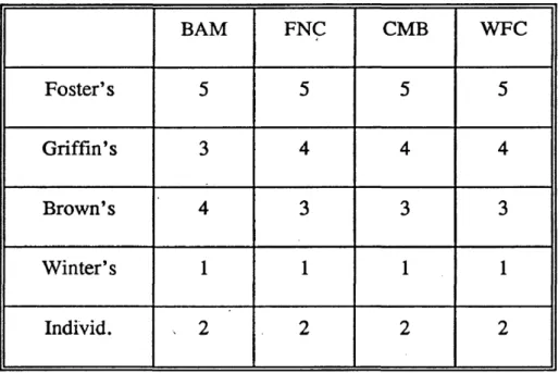
2. Individually developed models versus global ones: comparison with the models proposed by Foster, Griffin, Brown and Winter 47 Table no.Ill
Ranks attributed to the five models for BankAmerica, Citicorp, Chase Manhattan
and Wells Fargo 52
VI. Conclusion and recommendations 53 APPENDICES
Appendix 1
Standard deviations of the models 57 Appendix 2
Ranks attributed to the models by SAS RANK Procedure 59 Appendix 3
Number and percent of times the models were ranked 1 or 2 60 Appendix 4
Nonparametric tests for comparing the models 61 Bibliography
I. THE IMPORTANCE OF EARNINGS AND EARNINGS RESEARCH
Earnings are widely believed to be the most important information item provided in financial statements. Economic theory allocates the main role in directing resource allocation in capital markets to earnings information.
Accounting forecasting models have been used in auditing analytical review, in financial ratio analysis, in assessing corporate share value and in evaluating accounting changes. The beliefs regarding the importance of this accounting research vary widely. In the 1960s, issues of financial information usefulness were at the top of the research agenda. The Financial Accounting Standards Board introduced the issue of interim financial reporting and focused the earnings research literature of the 1970s on the usefulness of quarterly data in forecasting.
It is in the 1980s when the question of earnings information usefulness was most debated. The beliefs varied from saying that "when the capital markets err in predicting a firm’s earnings, the firm’s stock price typically moves in the direction of the error, and the magnitude of the stock movement is related to the size of the error," ( L.D. Brown, 1987, pp. 74) to saying that "the correlation between earnings and stock returns is very low, sometimes negligible, [..] suggest that the usefulness of quarterly and annual earnings to investors is very limited" (B. Lev, 1989, pp.21).
explain stock prices. Most of the studies continue the traditional time series models, developed in the seventies. These introduce structural changes or base the valuation models on time series representations. ARIMA models are used to detect potential structural changes by studying the residuals in the work of Lee and Chen (1990), while Ramakrishnan and Thomas (1992) develop the book value, market value and capitalized earnings models and base these models on various possible ARIMA processes.
The purpose of the present thesis is to focus on finding the time series properties of quarterly accounting earnings and comparing the performances of different models. Five different models will be examined from the goodness-of-fit perspective: ARIMA(1,0,0)(0,1,0) developed by G. Foster, ARIMA(0,1,1)(0,1,1) suggested by P. Griffin, ARIMA(1,0,0)(0,1,1) proposed by L. Brown and M. Rozeff, Winter’s exponential smoothing and an individually developed ARIMA model, specific for each company.
n . AN HISTORICAL DESCRIPTION OF EARNINGS RESEARCH LITERATURE
The earnings forecasting research began in the 1970s and is considered to have a stronger relationship with capital markets research since Foster’s work (1977). Three basic models for quarterly companies earnings have been developed. The later work in the field provides evidence in favor of one of these models. Each of the three versions employed ARIMA methodology to identify and estimate the parameters of quarterly earnings time-series models. The two major findings of these three models were (1) quarterly earnings may be described adequately as a multiplicative combination of two processes, adjacent quarter-to-quarter movements and annual quarter-to-quarter movements, and (2) firm-specific ARIMA models do not perform better in forecasting quarterly earnings than a basic ARIMA process underlying all companies income behavior.
The developments in the theory were encountered especially in the 1990s. Factors like structural change or the analysts’ earnings forecasts (Lee and Chen ,1990, Ramakrishnan and Thomas, 1992) were added to the basic ARIMA models.
The first of the three reference models for quarterly earnings forecasting was developed by George Foster, in 1977. Foster published "Quarterly Accounting Data: Time-Series Properties and Predictive-Ability Results" - a study of quarterly earnings, sales and expense series of 69 firms over the 1946-74 period. The author examined six
alternative models. The first two assumed a seasonal pattern in quarterly earnings, with and without drift. Another set of two alternate models ignored the seasonality and assumed a random walk (with drift) process. The fifth variant incorporated the other models, considering an (1,0,0)*(0,1,0) autoregressive, seasonally differenced series. A final alternative approach utilizes the Box-Jenkins methodology for identifying the process that generates each series. This last variant was previously analyzed by Nelson (1974) and Watts (1970). They illustrated that the analysis can lead to a diversity of models across firms when using finite samples, even when all the firms have a similar time-series behavior.
The solution suggested by Foster is to examine the predictive ability of the model on a set of observations not used for model identification and estimation. As underlined in the introductory part of the present study, the question of the seventies was if an interim financial report is to be required from firms. The existence of the seasonality in earnings time series had been, already recognized then and many models had been developed at that time to deal with this process. What the accounting research had to solve at that moment was the question: will investors be confused and mislead by the seasonal reporting, or do they know to adjust the information for the seasonality? Foster examines the predictive ability of the six alternative models in two contexts: (1) the ability to forecast future values of the same series and (2) the ability to approximate the capital market’s expectation.
combination in the 1962-74 period. A Friedman analysis of variance test is used to test the significance of the differences between the average ranks of the six models. Foster uses also the Mean Absolute Percentage Error and the Mean Square Percentage Error to evaluate the dispersion of the forecast errors.
What makes the Foster’s study particularly important for the history of accounting forecasts, as L.D. Brown underlines, is the introduction of capital market research in the earnings forecasting literature. Foster examines the association between capital markets indicators for each firm, and the sign of the unexpected earnings change. Because this regression is a strong one, he concludes that the aggregate market, when interpreting an interim report, adjusts for the seasonality in the earnings series. The study of George Foster ends, from the time-series perspective, with choosing the (1,0,0)*(0,1,0) ARIMA model as the most appropriate one in quarterly earnings forecasting.
The second ARIMA reference model for quarterly earnings was presented by Paul Griffin in "The Time-Series Behavior of Quarterly Earnings: Preliminary Evidence." The tentative four ARIMA alternatives that Griffin analyzes are different from what Foster before considered to be possible variants. He compares the following ARIMA models: (0,1,0)(0,1,0), (0,1,1)(0,1,1), (1,0,0)(0,1,0) (Foster’s), and (0,0,1)(0,0,1). The sample of firms included ninety-four companies listed on the New York Stock Exchange during the period 1958-71.
The criteria used by Griffin, in selecting the best model for describing the quarterly earnings, include the autocorrelation coefficients, the partial autocorrelation
coefficients and the Box-Pierce statistic. The conclusion of the study is that the first-order autoregressive model applied to four-period differences (the model developed by Foster) in quarterly earnings does not account fully for seasonality. Griffin considered that the stationary series, quarter-to-quarter differenced, have to include regular and seasonal autoregressive or moving average processes. The multiplicative first-order moving average ARIMA (0,1,1)*(0,1,1) model is suggested as the most appropriate for quarterly earnings forecasting.
The third model in the earnings literature was developed by Brown and Rozeff. Comparing the results of the previous two (Foster’s and Griffin’s) models with the proposed ARIMA (1,0,0)*(0,1,1), for a sample of fifty company’s earnings, Brown and Rozeff suggest that the latter performs better in forecasting longer than one-period ahead. In "Univariate Time-Series Models of Quarterly Accounting Earnings per Share: A Proposed Model," Brown and Rozeff use the most frequently identified ARIMA models in a previous study to test for the existence of the same underlying pattern for all the companies earnings per share numbers.
In a previous study, Brown and Rozeff examined fifty companies and found evidence for two Foster models, eleven Griffin-Watts models and fourteen Brown-Rozeff models. The rest of twenty-three companies were found to have different explanatory ARIMA processes. In their analysis, they reported only to Foster’s, Griffin’s and their own model. The diversity of the individually determined models might have appeared as a result of sampling errors. Therefore, the study tested the significance of the
performances of these single-firm models and the global models found earlier in the related literature. The Brown-Rozeff and Griffin-Watts models are found to perform better than the Foster one in estimating the firms quarterly earnings per share behavior. Brown and Rozeff s study continues by finding that in the long-term, the Watts-Griffin model’s forecasts follow a straight-line path as forecast horizon lengthens, but those of the Brown-Rozeff model follow a less steep, curved path.
The conclusion of the study is that the ARIMA (1,0,0)*(0,1,1) model is superior in terms of forecasting accuracy to the other analyzed alternatives, and should be used therefore as (1) a replacement for identification of individual Box-Jenkins models and (2) a benchmark model for evaluating security analysts’ or time-series models’ quarterly forecasts.
Several attempts have been made to improve the performance of the basic ARIMA models. Lee and Chen (1990) showed that these models can be enhanced by incorporating temporary, short-run and long-run structural changes. The authors of "Structural Changes and Earnings Forecasts," Lee and Chen, consider that the global model was preferred in modelling the stochastic structure of accounting earnings because structural changes were not included in the analysis. They state, "The parsimony in the global model makes it more robust to changes in the economic environment." (Lee and Chen, 1990, pp.94) Accounting earnings are decomposed in Lee and Chen’s study into two parts: (1) the stochastic process modelled as a multiplicative ARIMA process, and
approach on the residuals obtained by initially fitting an ARIMA model, with the assumption of no structural change.
Lee and Chen compare six models: the firm-specific model with complete control for structural changes, the firm-specific model with partial control, the firm-specific model without control and the three basic ARIMA models in the literature (Foster, Griffin, Brown). In Lee and Chen study, the statistical measures used for comparing the forecasting performances are the percentage of absolute forecast error and the percentage of squared forecast error. The ranks for the six models in the study are assigned considering 24 forecasts, and two statistical tests (the pair-wise rank test and the Friedman rank sum test) used to compare the models. The conclusion of the analysis is that "a well-executed firm-specific model with structural change adjustments outperforms the global models in forecasting the primary EPS of utility firms." (pp.96)
In "Earnings Forecasting Research: Its Implications For Capital Markets Research," (1993) Lawrence D. Brown presents a comprehensive historical look at the earning forecasting literature. He points out several studies in forecasting annual earnings of the companies, as well as research conducted in evaluating the analysts’ earnings expectation process, biases and sources of enhancements.
The earnings literature is very vast and includes several other approaches than the ones referred in this analysis. For the purposes of the present paper, the focus is on the literature review on the time-series models developed for describing quarterly earnings behavior.
m . COMPREHENSIVE PRESENTATION OF TIME-SERIES ANALYSIS USING SEASONAL EXPONENTIAL SMOOTHING AND BOX-JENKINS MODELS
This study compares model fitting for quarterly earnings per share numbers using Winter’s exponential smoothing technique and ARIMA processes.
1. Winter’s seasonal exponential smoothing
The smoothing methods generally include moving average models and exponential smoothing techniques. The first category starts with the idea of equally weighted observations, ending up using unequal weights, with moving averages of moving averages. The larger weights are given to the middle values of the past set of data, so that this group of models is useful for smoothing rather than forecasting purposes.
The exponential smoothing techniques imply exponentially decreasing weights as the observations get older. This weighing provides the advantages of moving average methods, with a faster response of the model to changes in data patterns. While the single exponential smoothing methods deal with stationary data, the double smoothing takes into account the trend (linear), but neither of these can forecast series with a significant seasonal component. Seasonal data are better smoothed using Winter’s method, which is based on three smoothing equations: one for stationarity, one for trend
and one for seasonality.
The equation of the forecast can be written:
F»m ~ (S, + b,m)1,-L.„
where L is the length of seasonality, b is the trend component and I is the seasonal adjustment factor.
The main model represented by this equation is a double exponential smoothing, which has been transformed to handle the seasonality:
s r « A +(i . a ) (st l+bt _x) Vl
b ' - y + (1 - y ) 6,-1
/(. p 5 +(l_p)/(1
The first equation is the overall smoothing equation, and, together with the second equation, adjusts the series for a linear trend. This adjustment is different from Brown’s double exponential smoothing since it allows the trend to be smoothed with another parameter than that used for the original series. The last of the above three equations is used for the seasonal smoothing. The St values are averages of the series that do not include seasonality, as opposed to the Xt values, which do include it.
The process of initialization is more difficult in Winters’ method than for other exponential smoothing techniques. For Winter’s method, properly chosen weights are of critical importance in generating reasonable results. There are several factors to consider
when choosing weights. The more variance in the data, the lower should be the weight attached to the most recent observation. Another factor to consider is how quickly the time series is changing. If the series changes rapidly in trend (has an exponential increasing rate for example), relatively more weight should be placed on the most recent observation. The seasonal weight applied to the data varies according to amount of seasonality observed and irregularity of the seasonal factor.
The present analysis will focus on individually developed ARIMA models and compare those with global ones. Winter’s method will be considered with a general model for all companies. Therefore, the SAS default values will be used for the weights in Winter’s model, weights that are dependent on the trend value only. This default weights are .25 for the seasonal and trend adjustment and (1-0.8**(1/trend)) for smoothing the constant. The SIGMA option in the SAS FORECAST procedure provides a measure of the Root Mean Square Error of the Winter model.
2. ARIMA(p,d,q)(P,D,Q) models for the analysis of time-series
Another approach in the analysis of time-series is developed in the class of models known as ARIMA(p,d,q)(P,D,Q) models. The main concept is to consider the actual values of the series, from which the trend is eliminated first by d differencing of data, as a consequence of the last p values of the same series without trend, and of a series of q error terms.
Using the chosen notations, the general model, without taking into account the seasonality, is:
(1-<|>1B -c|>2B2-...-<|>/,B'’)(1 -B )‘'>-< -
8 + ( l - e iB - e 2B2- . . . - 0 sB 9) e (
where B is the backward shift operator (BXt=Xt,1).
For the seasonal time series, the model, A RIM A C pjd^^D jQ )8, detects seasonality from the differenced data in a manner similar to that applied for recognizing the AR and MA processes.
The process of fitting an ARIMA model to the data involves the following steps:
1. Identify the model. In this step, the concepts of autocorrelation, partial correlation and differencing help in recognizing the pattern of the data and in adopting
an appropriate model. The autocorrelation coefficient between Xt and Xt_k is defined:
cov{Xt,Xt_k)
The autocorrelation coefficients follow a normal distribution, with the standard _1_
\fn
error a - — ji - N - d • This allows the developing of a comprehensive statistic,
used in diagnostic checking — the Box-Pierce Q statistic, Q - n Y ,rk > which is
k-l
distributed approximately as a chi-square statistic with (m-p-q) degrees of freedom (m is the maximum numbers of lags considered).
2. Estimate the parameters in the tentative model and test the appropriateness of the model (diagnostic checking). Most of the statistical software packages will provide
the results of the estimation, once the model is defined. Diagnostic checking is done by: a), studying the residuals, to see if any pattern still exists. This can be done by analyzing the mean percent error, which indicates the presence of bias in the residuals, or by checking the autocorrelations of the residuals (including the comprehensive measure that is the. Q-statistic)
b). studying the sample statistics of the estimated model, or the closeness- of-fit statistics. Over the past years, many studies have been conducted to find the best method in terms of accuracy, for a certain kind of data. This is also the purpose of the present study, since its aim is to find the most appropriate forecasting technique for earnings per share quarterly data. The criteria that the present study will use is the standard deviation (root mean square error) of the series estimated using various models.
Several other measures of closeness-of-fit of a model have been developed. In a recent study, J. Armstrong and F. Collopy evaluated several measures for making comparisons of errors across time series. The following table provides their rating of the error measures:
E rror Reliability Construct Outlier Sensitivity Relationship
measure validity protection to decisions
RM SE poor fair poor good good
MAPE fair good poor good fair
MdAPE fair good good poor fair
GMRAE fair good fair good poor
The error measures used in the study conducted by Armstrong and Collopy are: RMSE (Root Mean Square Error), MAPE (Mean Absolute Percent Error), MdAPE (Median Absolute Percent Error), GMRAE (Geometric Mean of the Relative Absolute Error) and MdRAE (Median Relative Absolute Error).
The present analysis uses the Root Mean Square Error because it is the most widely used statistic and because it is the only measure computed by the SAS procedures used by this study.
3. Use the model to forecast the series and analyze the forecasting errors. The primary use of forecasting errors is in generating confidence intervals around the forecast
values. The SAS ARIMA procedure provides two methods for obtaining forecasts of a univariate time series, depending on the method specified in the estimation step. Because the present analysis focuses on goodness-of-fit rather than on accuracy of the models, this ARIMA step is not necessary.
IV. SAMPLE SELECTION AND DATA DESCRIPTION
The study includes a sample of twenty firms from five major and diverse fields: homebuilding, food processing, machine tool, chemical and banking. Each of these fields is represented by four firms that have been listed in The Value Line Investment Survey
with quarterly reported earnings per share during 1977-1993. Thus, the time series have 68 quarterly observations.
The sample was intended to have diversity between and within the industries. Every one of the five industries was expected to have its own stochastic pattern. The homebuilding field is expected to have the most seasonality. The previously developed ARIMA models reviewed in the earnings literature concluded that most of the companies from all the sectors have a seasonal component. This study is expected to find, for the latest time period, less seasonality in food processing because of increasing external trade. The chemical industry will reflect the cycles in oil prices. All the other industry groups will have an affect on banking field. Because of the differences in the financial year structures of the companies, the affects of other field’s fluctuations in earnings on bank’s accounts will probably be offset.
More than twenty firms from the groups considered met the criterion. Five homebuilding corporations, five from the chemical industry, five from the machine tool sector, 14 from banking, and 23 from the food processing industry constitute the
population. Because the selection for homebuilding, chemical and machine tool industries was limited, the present study selected four from each of them. Even when the company was present for the time period of the present study, some had too many unreported values (Giddings&Lewis, from machine tool industry) and some had a big administrative change (Webb Corp., from homebuilding industry). The other two fields, banking and food processing, could have had more than four units selected. The sample size of 20 determined the option of four firms to be included from the other two industries also.
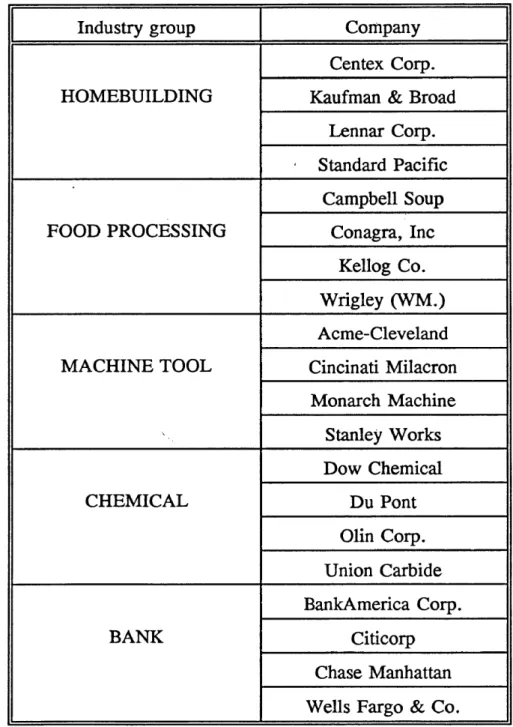
The Value Line Investment Survey lists the corporations in alphabetical order. Therefore, this study included in the sample firms selected on the basis of a selection fraction (this fraction was chosen equal to two for banking and equal to five for food processing). Table I presents the twenty firms included in our examinations.
It is important to note that inferences drawn from this study apply specifically to the five fields selected and to a sample of "survivor firms" (firms that have been in business for the 1977-93 time frame).
Some difficulties were encountered in collecting the data; companies have different fiscal year structures and missing observations appeared in the case of three companies (four from 68x4). Since SAS ARIMA does not work with missing observations, the problem was solved by using the SAS procedure EXPAND, which interpolates the missing values. This procedure (EXPAND) is recommended by SAS documentation as the best method for dealing with missing observations. The earnings per share series for each industry group are presented in Figures no. 1-5.
Table I Companies included in the study of quarterly earnings
Industry group Company
HOMEBUILDING
Centex Corp. Kaufman & Broad
Lennar Corp. * Standard Pacific FOOD PROCESSING Campbell Soup Conagra, Inc Kellog Co. Wrigley (WM.) MACHINE TOOL Acme-Cleveland Cincinati Milacron Monarch Machine Stanley Works CHEMICAL Dow Chemical Du Pont Olin Corp. Union Carbide BANK BankAmerica Corp. Citicorp Chase Manhattan Wells Fargo & Co.
Fi
gu
re
no
.1
Ea
rn
in
gs
pe
r
sh
ar
e
in
ho
m
eb
ui
ld
in
g
5 6661 S' 1661 S 0661 S 9861 Q-Q861 Q>861 5X861 5 1861 8'086l 5'6Z6l 5 8^61 b'ZZ.6L u_ CL CO LU mo
Pa
ge
18
Fi
gu
re
no
.2
Ea
rn
in
gs
pe
r
sh
ar
in
foo
d
pr
oc
es
si
ng
Pa
ge
19
s> CO u 0.-0 </> .E 05
_
.E oE 2
u j | 2 ^2 CDc E
2> o3 • — .05 i £661 ££661 S' 1661 8f&61 rT 0 6 6 L 86861 S’886 i s m v 8 986 L 6 886L_ * 8 8861 S 1861 8*0861 8*6A6l 8*886 L 8*886 L o CM Q> 05 CO CLFi
gu
re
no
.4
Ea
rn
in
gs
pe
r
sh
ar
e
in
ch
em
ic
al
i
nd
us
tr
y
5 6661 5-^661 8u66L 5’6861 87861 b 9861 8‘886l 8>86l 8186 L 9 686 L 9' 1861 9 0861 8 6/161 9’8/6L 8 7 /6 i z _ J o o Q O OPa
ge
21
8> CO Jc tn i_ O) Cl <o 05
(/)
e r* C E co CO -Q UJ E W ■ o c S> 3 05 5*665 L 5;.Q6.6l Q66J 5*6861 6861 5'886l 8861 55861 5 586 L S'286L 5' L86 L 5 086 L 5 6561 5 856 L 5 5 / 6 1 o m 5 oo
< CD CM CM <D 05 CO £ LV. RESEARCH RESULTS - PRESENTATION AND CRITIQUE
This section of the paper will present the reasoning that led to the decision to adopt a specific ARIMA model for describing every company’s earnings per share numbers. The review of the earnings literature pointed out that several studies have concluded global time-series models may perform as well as the individually developed ones. The second part of this chapter presents a comparison between the group of individually estimated models against the proposed global models.
1. Description of corporate earnings per share using Box-Jenkins approach 1. Homebuilding
Some results for firms are discussed in the following section. The first field included in the analysis is homebuilding, represented by four companies: Centex Corp., Kaufman&Broad, Lennar Corp., and Standard-Pacific.
CENTEX CORP. (CTX)
Centex Corporation grew, in the time period covered by our study, from a classified ’'major” to "the largest" home builder in U.S. The financial indicators listed by The Value Line Investment Survey show an increase over the company’s financial strength from C + + to B + , and a greater stock price stability. Centex Corp.’s earnings predictability improved during the time of our analysis.
The earnings per share series fluctuates mostly between $0.4 and $0.9, with an average of $0,627. One high peak appears in the second quarter of 1980 (fiscal year ends March 31 for Centex Corp., therefore this would be the last financial quarter of 1979). When analyzing the financial situation of Centex Corporation, one has to consider the lag between orders and deliveries. Hence, the peak of March 1980 derives from the situation of December 1979 orders. In 1979, besides spending 2.5 times more than in the preceding year on exploration and development, other important changes occurred: the company sold an interest in some energy properties to ease the financial strain and a gas processing plant was put into work. Since the value in March 1980 is 4.40 times larger than the mean of the working series, these data were identified without this extreme value. As explain in the previous chapter, this missing value will be interpolated by the SAS EXPAND procedure. The standard deviation of the original series decreased from .329 to .200. Analysis was continued without this outlier.
In the identification phase of the Box-Jenkins procedure illustrates first two autocorrelations (ac) statistically significant and partial autocorrelations ipac) of lag 1, 6 and 7, outside the confidence interval. The series needs therefore no differencing and has no significant seasonality. A first-order autoregressive parameter and two moving averages were introduced in the estimation phase. Residual analysis shows no significant
ac's or pac's. The standard deviation of the original series is improved by 42.5 percent and the diagnostic checking using chi-square tests shows no remaining pattern in the residual series. ARIMA(1,0,7) was selected for the Centex Corp. quarterly earnings per
share numbers. The mathematical model estimated for Centex Corp. is (1 - 0.61 IB1 )yt - 0.602 + (1 - 0.427B6 - 0.536B7) e g
KAUFMAN & BROAD (KB)
Kaufman and Broad, Inc. started as a homebuilding and life insurance company, then changed into a building company in 1986. The financial part of the firm became the new Broad, Inc. Since the results of the analysis might have been affected by this change, the model was developed for both time periods: 1977-1993 and 1986-1993. For the time span of our study, as shown in The Value Line Investment Survey, the company improved its financial strength from C + to B + , the earnings predictability increased three times, but the stability of the stock’s price has been evaluated as decreasing. The mean of the series is $0,298, with a standard deviation of $0,231.
Identification of the earnings per share series, in the case of Kaufman and Board, shows decreasing, statistically significant ac’s of lags 4, 8, 12 quarters and relatively large, pac’s of lags 4 and 8. The first order pac is also statistically significant. We introduced one regular moving average (lag one) and one seasonal moving average (order one) parameters, reducing in this way by 11.25 percent the standard error of the data. Estimation of the new model shows that all selected parameters are statistically significant (conclusion inferred from the t-values listed by SAS). If another seasonal autoregressive parameter (order two) is added to the model, the standard deviation decreases by another 5 percent. The correlation matrix has in one high member (.492) in the last variant,
which suggests an overfitting of the model. Because of the change that occurred in the company’s organization, the series was also analyzed for 1986-1993. Identification phase for the 34 observations indicate large ac's of order 1 ,2 , and 4. This pattern of the data suggested ARIMA(1,0,0)(1,0,0) to be the model that describe the series since 1986 (the standard deviation of the series since 1986 is reduced, with this transformation, by 21.65 percent), as well as from 1977 till 1993. This is the reason we have decided to work with the same sample as for the other nineteen companies, and the model selected for Kaufman&Broad is:
yt - 0.291 + (1 - 0.34IB 1) (1 - 0.409B4) e f
LENNAR CORP. (LEN)
Lennar Corporation is a planner and builder of moderately priced single and family housing in Florida, Arizona and Michigan. The company has the enviable position of being the largest homebuilder in Florida. The increasing trade with Latin America and the preferences among retirees make a very good market for this particular industry. Although the company’s financial strength is not considered to have increased substantially, the earnings predictability and stock’s price stability are three times higher now than at the beginning of the period presently studied. One can distinguish several temporary peaks and troughs in the company’s earnings per share figures. It is expected that Lennar will have a record year of share profits in 1994, due to the contracts carried
over from the end of the 1993 fiscal year, the expected stability of mortgage rates and the rise in the home prices.
The identification phase of the ARIMA procedure describes a nonstationary time- series of earnings per share for Lennar Corp. Autocorrelations decrease very slowly and the first-orderpac is high: .735. Therefore, we identified the first-order differenced data. Differencing resulted in a smaller standard deviation of the series: .148, from .211 in the original data. In the new identified model, there is one significant ac of order one and a nonzero pac of lag one. Therefore, in the next step, a moving average parameter of lag one was added to the estimation phase. The t-statistic proves the significance of the new parameter and the autocorrelations of the residuals show no remaining pattern in the data. The study arrived at the ARIMA (0,1,1)(0,0,0) model for the Lennar Corp. earnings per share numbers shown below:
( l - B ) y r- ( l - 0 . 2 9 9 B 1) e f
STANDARD-PACIFIC (SPF)
Quarterly earnings per share follow a cycle at Standard-Pacific over the time span studied. After demonstrating relatively high numbers in 1978, the company showed a decline in earnings until 1982, when the next expansion began and lasted through 1989- 1990. The decline that began in 1990 was very rapid and dramatic. The fall in 1982 was caused by high interest rates and low house prices, while the 1989-1990 boom was triggered by the climbing home prices in California. Due to the state’s tightening
development regulations minimizing the supply of available homesites, Standard-Pacific, which has been able to maintain a large supply of homesites, increased its profit margins substantially. The favorable situation changed very much in the nineties, the decline continuing at the end of our data set. In an effort to make the shares more attractive, Standard-Pacific converted from a master limited partnership to a corporation in December 1991.
The identification phase of the ARIMA procedure defines a nonstationary series, since the ac’s experience slow decline. Differencing the series reduces its standard deviation by 32.87 percent. The fourth pac and ac and the first-order one suggest a seasonal moving average parameter and a regular first-order one should be included in the model. Estimation phase proves the statistical significance of the selected parameters ( the t-values are high) and the residual analysis shows no remaining pattern in the new series. The selected model for describing quarterly earnings per share for the case of Standard-Pacific is the ARIMA(0,1,1)(0,0,1):
(1 - B) y, - (1 - 0.297B1) (1 + 0.524B4) e,
2. Food Processing
Stable in comparison with the series from other sectors, the food processing industry is represented in this study by Campbell Soup, Conagra, Inc., Kellog Co., and Wrigley.
CAMPBELL SOUP (CPB)
Campbell Soup is a leading manufacturer of canned soups, spaghetti, fruit and vegetable juices, and frozen foods. At the beginning of the time span of the study, Campbell was the largest domestic and Canadian manufacturer in this field. As viewed by The Value Line Investment Survey, the company’s financial strength slightly decreased, from A + + to A + during the past fifteen years, while the earnings predictability dramatically dropped together with the stock’s price stability. After the beginning of the 1980’s, when Campbell Soup’s earnings per share reached a peak (1981 quarter 3), the decline started. The bottom point of the decline was the negative $0.79 reached in the second of 1989. This sharp decrease was related with problems in the founder’s family (the founder’s son died and the company changed the head). Earnings per share improved at Campbell during the nineties. Campbell Soup is expected to continue its growth due to improvements in international operations (restructuring in Europe) and to a acquisition of a majority stake in Amotts.
The analysis of the original series for the earnings per share numbers in the case of Campbell Soup shows nonstationary data. Large first-orders ac's that decline to zero after the lag of eight and high pac's made us consider a first order difference as necessary. The differencing reduced the series’ standard deviation by 23.88 percent, leaving large ac's of lags 1, 2, 12, and a high pac's of lag 1, 2, 3. We estimated the model with one autoregressive seasonal parameter of lag 12 and one regular moving
average. The model chosen for the Campbell Soup earnings per share numbers is ARIMA(0,1,1)(3,0,0):
(1 -0.352B12) ( 1- B ) y r (1 -0.631B1) e f
CONAGRA, INC. (CAG)
Described as "a diversified food processor" at the beginning of the time span of the study, Conagra is now classified as "the nation’s second largest food processor." The company has demonstrated remarkable consistency in expanding sales and profits,with only two down years in share earnings since 1977. The earnings predictability index increased. Internal growth and acquisitions made this situation possible. Conagra acquired Armour Food Company in 1983, and recently joined with Kellogg to create several
Healthy Choice cereals and purchased a new section of frozen foods. Changing tastes and increasing concern about fat in American diets account for the larger numbers in earnings per share at the end of 1979.
Analysis of the results from the identification phase of the S AS procedure reveals significant ac’s of lags 1, 2, 4, 12 and the correspondent pac's. Several combinations of regular and seasonal parameters were introduced and the autoregressive parameter of order one and two, and a seasonal moving average of order three finally included in the selected model. The t-tests for the three parameters are significant and the standard deviation of the original series is reduced by 31.64 percent. The residuals correlations indicate no remaining pattern in the data. One might argue that the model is overfitted,
since we have a high correlation between the autoregressive parameters. After exploring other possibilities, the ARIMA(2,0,0)(0,0,3) model was selected for the earnings per share numbers of Conagra, Inc.:
(1 - 0.28451 - 0.386B2)yt « 0.511 + (1 + 0.638B 12) e ,
KELLOGG CO. (K)
During 1977-1993, the time period covered by this study, Kellogg succeeded in remaining the world’s largest manufacturer of ready-to-eat cereals, although its domestic market share declined slightly (with 5 percent). There are several indicators of consistency at Kellogg during the time: the company’s financial strength was steadily A + + , the earnings predictability varying very little around 90. The company is appreciated as very strong financially and recommended for risk-averse investors. For the near future, Kellogg is expected to do well especially due to the external markets, while the domestic sector might be affected by the price cuts announced by General Mills.
The original series, analyzed with ARIMA, shows four large first orders ac* s, while the first two and the fourth pac' are also high. The partial autocorrelation of lag five is statistically significant and, even though this lag does not do much in explaining and forecasting the series, the corresponding moving average was introduced and improved the model. Estimation phase has been conducted with a first-order autoregressive parameter, a first-order seasonal one, and a moving average of lag five.
The standard deviation of the original series has been reduced by 34.74 percent and the chi-square tests detect no remaining pattern in the series. ARIMA(1,0,5)(1,0,0) has been selected to describe the earnings per share for the Kellogg Co.:
(1 -0.64651)(1 -0.621B*)yt -0.593 + (1 - 0.3375s) e,
WRIGLEY (WM.)
Earnings per share figures at Wrigley, the world’s largest chewing gum manufacturer and seller, show a fairly constant, though decreasing pattern. The company’s sales grew during the last twenty years, but due to the fact that almost half of this volume is realized overseas, the growth has been partly offset by the strengthening of the U.S. dollar. At the beginning of our time span, Wrigley faced increased costs for raw materials. However, Wrigley has not raised domestic prices and this fact boosted the market share, but declined for this reason the profit margins.
The original series has a decreasing trend, shown by SAS identification phase in the long lag of significant pac’s and very large first-order pac. After differencing, the mean of the series is negative (the trend is decreasing) and the new identification step reveals large first and second order ac’s and pac’s, and high ac and pac of lag four. The estimation phase with two regular, first and second order moving averages, and one first order seasonal moving average proves that all parameters are statistically significant ( the t-values are large). The residual analysis concludes that no significant pattern exists in the new estimated model. Wrigley’s earnings per share during the time period between
1977 and 1993 can be described with ARIMA(0,1,2)(0,0,1):
(1 - B)y, - (1 - 0.298B1 - 0.281B2) (1 + 0.32 IB4) e,
3. Machine Tool
The most fluctuating series in this study are the ones representing earnings per share in machine tool industry. The nonconstant variation caused two of the series to be analyzed in the logarithmic transformation. Selected companies in this field are Acme- Cleveland, Cincinatti Milacron, Monarch Machine, and Stanley Works.
ACME-CLEVELAND (AMT)
Acme-Cleveland has been constantly appreciated with a grade of B for financial strength as rated by The Value Line Investment Survey over the time period between 1977 and 1993. However, for the same time frame, the large producer of machine tools, experienced sharp declines in stock’s price and earnings predictability points of view. At the beginning of the period, the company was characterized by large variability in earnings per share numbers and by several shocks including the changing of presidency in 1980, and strikes in March 1985. Capital additions made the debt and interest charges high and the depreciation expense rise at a higher-than-normal rate. Recently, orders at Acme-Cleveland increased because of the large demand for inspection systems and telecommunications test products. With a lower level than at the beginning of the period, earnings per share look more stable in the nineties.
variant suggest that there is a nonstationarity in the variance of the data (the model is heteroskedastic). The logarithm and the identification of the new series confirms this hypothesis. The new ac’s are high for the first four lags and so are the pac*s of lag 1, 2, 4, and 6. Estimation was conducted with one regular autoregressive parameter, one seasonal, and one moving average of order six. All the parameters are significant and the autocorrelations of the residuals are statistically zero. Standard deviation of the original (log) series was reduced by 19.78 percent. ARIMA(1,0,6)(1,0,0) is chosen for the Acme- Cleveland earnings per share:
(1 -0.334B ')(1 -0.235fi4)log(y,) --1.061+ ( 1 +0.307B«)e;
CINCINNATI MILACRON (CMZ)
One of the top suppliers of machine tools and plastic processing machines, Cincinnati Milacron Inc. displays a very large variance in earnings per share during the 1977-1993 period. Demand fluctuations for metal and plastic cutting machinery affected the company because of its leading position. Although other parts of the company’s businesses did very well in this time, the weakness of the machine tool segment, which counts for 65-70 percent of total sales, eclipsed the good news from the other sectors. Large orders heavily influence the company’s accounts very much. The company’s financial strength was steadily evaluated with a B rating by The Value Line Investment Survey during this time, but earnings predictability decreased eight-fold.
Earnings per share have been fluctuating little between 1977 and 1982, when they are also positive, and started to have a large variation, including large negative numbers, since 1982. The logarithm of the data is used and this transformed the series one stationary in variance. The model has three significant pac's and four non-zero first ac's. We estimated the new model, with the additional introduction of three autoregressive parameters. Residual analysis displays no remaining pattern in the data and the model selected is ARIMA(3,0,0)(0,0,0):
(1 -0.150B1 - 0.137B2 - 0.277R3) log(yf) - -1.203 + e f
MONARCH MACHINE (MMO)
Monarch Machine is a rather small but financially sound manufacturer of manual and computer controlled turning machines and vertical machining centers. After a period of increasing earnings per share numbers at the beginning of the time period of this study, the company shows constant small numbers until 1993. "This company’s results are rarely in phase with the general business cycle," says The Value Line Investment Survey. Many of Monarch Machine machine tools take several months to build, so, like all machine tool industry, the accounts of the Company are affected by these backlogs.
The identification phase of Box-Jenkins analysis resulted in a series with ac's that decline to zero after four lags and a .713 first-order pac. Therefore, after differencing, the new series had one high ac and the corresponding first-order pac.
a standard deviation with 30.80 percent smaller than the original series and statistically zero autocorrelations of the residuals. ARIMA(0,1,1)(0,0,0) was the model selected for the data in the case of Monarch Machine Tool Company:
( l - 5 ) y r- ( l- 0 .4 4 9 5 1) e f
STANLEY WORKS (SWK)
The consistency in Stanley Work’s performances increased its earnings predictability and price growth persistently in the time period considered in this study. Stanley Works is the world’s largest manufacturer of hand tools. It purchased Mac Tools at the beginning of the period analyzed, entering the only major hand-tool area in which the company was not a factor. This investment and other that followed (the acquisition of a division of Textron in 1985 and the purchasing of the hand tool manufacturing business of Peugeot Group in 1986) slightly affected the company’s financial strength. Stanley Works managed to be profitable despite the changing climate of the machine tool industry. Presently it is involved in external markets like Australia and the Far East, in addition to the domestic sector.
The identification phase of the ARIMA analyzed the original series and pictures two significant ac's for the first lags, and a decreasing pattern in the ac's of lag 4, 8, 12, 16. The first two and the fourth pac's are high. The model was estimated after introducing a first-order regular autoregressive parameter and one seasonal one. The standard deviation was reduced by 21.37 percent and there is no significant correlation
of the residuals. There is a significant correlation between the selected parameters, but the performance of the model significantly improve. The selected ARIMA(1,0,0)(1,0,0) model has the following equation:
(1 - 0.742B1) (1 - 0.820B4)yt - e f
4. Chemicals
The chemical industry displays, through all its exponents, a cycle in the earnings per share numbers more than any other of the industries examined above. It has a peak in the second quarter of 1978, a trough in 1980, quarter three; a peak in 1981, quarter two, a trough in the fourth quarter of 1982, a local high in 1984 quarter two; a peak in
1988 quarter two; and the latest low in the first quarter of 1993. The cycle is probably related mostly to the price of oil.
DOW CHEMICAL (DOW)
At the beginning of the period considered by our study, despite the recession of the early eighties, Dow Chemical, at that time the U .S.’s second chemical producers, was following its ambitious plans of capital spending. The company’s sales structure, with about 60 percent of its operating income from abroad in 1985, was favored by the decreasing value of the dollar and lower oil prices in the mid-eighties. Higher prices, modest volume improvements and increased productivity made the earnings in 1988 and
1989 excellent. The down-swing in the later years, observed in all companies from his field included in the study, is mainly due to excess industrywide capacity and poor
demand in a sluggish economy. Dow Chemical has been very consistent during 1977- 1993 from the perspectives of financial strength and stock price stability, but decreased slightlyin earnings predictability.
The analysis of the original series shows a slowly decreasing pattern in the ac's and a very high (.84) first-order pac. We therefore took the difference of the data and arrived at a model with significant first and second order ac's and pac's. Decreasing, high ac's of order 4, 8, 12, and 16, and large fourth lag pac suggest a seasonal autoregressive parameter. Estimation was conducted with a moving average of order one and a seasonal, first-order autoregressive parameter. Standard deviation in the series was reduced by 48.44 percent and the residual analysis shows no remaining pattern in the data. The ARIMA(0,1,1)(1,0,0) model for the Dow Chemical’s earnings per share pattern is:
(1 -0.380B4)(1 - 2?)yf- ( l -0.318B1) e f
DU PONT (DO)
While the cycle of the chemical sector can be clearly seen in the Du Pont earnings per share numbers, the company’s accounts have a supplementary pattern. Du Pont is the largest chemical company in the U.S. Its products include oil, natural gas, gasoline, agricultural chemicals and other specialties. The company’s earnings were very cyclical until 1981, when Du Pont merged with Conoco in order to dampen the oscillations generated in chemical industry. This hope held at the end of 1982, when the bottom
The graphical representation of the autocorrelations of the original series, indicates large first-order ac and pac, large ac's and pac's of order 4 and 8. The model as estimated after introducing the following parameters: first-order regular moving average, seasonal autoregressive parameter of order 1. The t-values validate these parameters (3.21 and 3.62, respectively) and the standard error of the original series is reduced by 14.88 percent. Residual analysis shows no remaining pattern in the data, except for the relatively high autocorrelation of lag 14. The presence of the lag of 14 in the model decreases the standard error of the series by another 7 percent, but this lag is not useful for forecasting purposes. Observation 14 reflects probably an irregular fluctuation (1989 quarter two is the peak of the Olin’s earnings per share series). ARIMA(0,0,1)(1,0,0) is the model selected for Olin Corp. series:
(1 - 0.412£4)y, - 0.773 + (1 + 0.370B1) e f
UNION CARBIDE (UK)
Earnings per share decreased sharply at Union Carbide in 1982 and after that partly recovered only for 1989. The second largest U.S. chemical producer sold parts of the business during the time span of our analysis. In some cases, selling and concentrating on a narrower area proved successful, but only for a short time (the selling of the battery unit in 1985 was followed by an increase of the earnings per share numbers and then by a large decrease). Union Carbide’s earnings have been affected a large part of this time span by a conflict related to a leak in India. This Bhopal case has taken big
bites from Union Carbide’s earnings per share since 1984. At the end of 1988, Union Carbide was ranked by The Value Line Investment Survey the highest company for year- to-year relative price performance. As Value Line analysts warned at that time, that increase had much to do with negative earnings comparisons. Union Carbide divided from its industrial gas segment in 1991 and the insufficient observations since that event make the company hard to forecast.
The negative trend existing in the data is confirmed by the pattern of the autocorrelations ( the ac's decrease to zero after five lags) and the negative mean of the differenced series ( which shows the decrease). Differencing arrived to a model with a significant ac of order 8 and the corresponding pac. We estimated therefore the differenced series with one moving average parameter of order 8. The new model reduced the standard deviation of the original series with 55.34 percent and has no other significant pattern in the autocorrelations of the residuals. Selection was made for ARIMA(0,1,0)(0,0,2) to describe the earnings per share of Union Carbide:
( l- £ ) y ,- ( l- 0 .3 0 9 J ? 8)e,
5. Banks
Earnings per share in all four banking corporations selected by this study reflect an unusual drop in the second quarter of 1987. The loss was due to a supplementary loan loss provision for Third World debt and affected the entire U.S. banking. Since that was an external shock to the data, the analysis in this study removed the unusual observation
in the second quarter of 1987. This elimination reduced the standard deviation of the series with 33.82 percent (BankAmerica Corp.), 50 percent (Citicorp), and 22.80 percent (Wells Fargo & Co.). Data for Chase Manhattan had another extreme value for the third quarter of 1989: -12.45 compared with an 1.425 on average. The elimination of this value and of the one for the second quarter of 1987 reduced the standard deviation of the Chase Manhattan original series with 47.38 percent.
BANKAMERICA CORP. (BAM)
BankAmerica Corp. holds Bank of America, which used to be the largest bank in U.S until 1990, when it was taken over by Citibank. The corporation had a red ink earnings per share year in 1985 and at that time, the only solution to recovery was seen as a takeover proposal for BankAmerica. A merger became a fact at the end of 1991 when BankAmerica joined Security Pacific. The merger proved positive for the earnings per share numbers. This favorable situation is expected to continue, due to the boost in the Californian economy brought by the 1994 earthquake (where BankAmerica has most banks).
ARIMA analysis started with identification of the original series. Large second and fourth order acs and pacs determined the estimation phase to be performed including one moving average parameter of order two and one seasonal autoregressive parameter of order one. The t-values are 3.62 and 4.22 respectively, which, for 65 degrees of freedom, imply statistically significant parameters (the critical value for .05 level of significance is 1.98). Correlation check of the residuals shows no remaining pattern in
the data and the standard error of the original series is reduced by 20.2 percent. The ARIMA(0,0,2)(1,0,0) was selected to describe quarterly earnings per share for BankAmerica Corp:
(1 - 0.48 IB4) 0.642 + (1 + 0.429B2)e,
CITICORP (CCI)
Citicorp, the largest banking company in the United States, owns Citibank, the biggest American bank. The company began with proving itself profitable within foreign countries and across international boundaries, both in consumer and commercial business. A good year for Citicorp’s earnings per share was 1983, when the company was appreciated as having "a bright future" by analysts from The Value Line Investment Survey. Given the weak economic climate of the nineties and especially due to the illiquidity of many commercial real estate markets, Citicorp counted negative earnings per share in 1991. The recovery is already taking place. Citicorp’s long-term strategy is to have a strong presence in relatively underserved developing nations that are expected to grow much more than the U.S. in the next few decades.
The identification phase of the ARIMA procedure reveals a stationary series, with no seasonality and large first three ac's and pac's. Estimation of the first-order autoregressive parameter and third-order moving average reduces the standard deviation in the original series by 25.55 percent and leaves no pattern in the autocorrelations of the
residuals.
ARIMA(1,0,3)(0,0,0) is the model selected to describe time series behavior of quarterly earnings per share for Citicorp:
(1 - 0.49651 )yt - 0.947 + (1 + 0.39551 )e ,
CHASE MANHATTAN (CMB)
The Chase Manhattan Corp. owns The Chase Manhattan Bank, the sixth largest banking holding company in the U.S., based on,assets at the end of 1992. Earnings per share at Chase, for the time period of this study, show two extreme values that have been eliminated as outliers. The company’s good performance at the beginning of 1982, despite all the losses from loans in Latin America, were due to the introduction of new money market accounts. Negative numbers in 1989 and 1990 are associated with changes in loan loss provisions. Chase is appreciated as decreasing by The Value Line Investment Survey in terms of earnings predictability and financial strength, for the time period of the study.
The original series exposes two significant ac's and one large pac. Introduction of a first-order autoregressive parameter in the estimation phase of ARIMA reduced the standard error of the original series by 6.8 percent and the only significant lag left in the residuals is the tenth one. A moving average of order 10 included in the model improves the standard error by another 8 percent. The tenth lag is not very important in forecasting. The study will consider ARIMA(1,0,0)(0,0,0) the model for the earnings per
share pattern at Chase Manhattan:
(l-0 .3 9 1 £ 1) y , - 1.421 + «,
WELLS FARGO & CO (WFC)
Wells Fargo owns Wells Fargo Bank, which has gone from the 11th largest bank in U.S. at the beginning of our study to the seventh one according to 1993 assets. Besides the loss encountered in all banks earnings per share in the second quarter of 1987, Wells Fargo’s is a relatively stable one.. The only red ink earnings per share number was reported in the last quarter of 1991. The loss in the last quarter of 1991 is related to an increase in Wells Fargo loan loss provisions, following a real estate examination by the bank regulators. The reason for the large increase in loan loss provisions was a reevaluation of the bank’s commercial real estate portfolio, that was seriously hurt by the poor economy in California, the main place of business for Wells Fargo.
One statistically significant ac of order two and tw large decreasing pac's in the original data identification determined the inclusion of a second-order autoregressive parameter in the estimated model. The parameter proves statistically significant and the standard error in the data reduces by 11.5 percent. No remaining pattern is shown by the residual analysis. The ARIMA(2,0,0)(0,0,0) is selected for quarterly earnings per share at Wells Fargo & Co.:
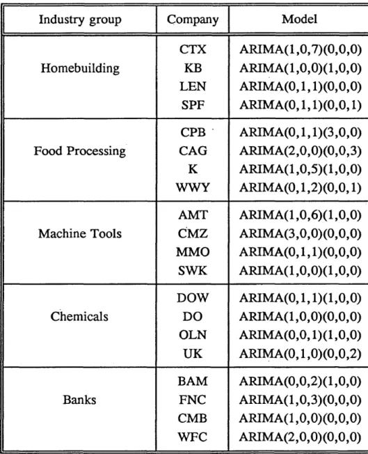
Table no. II Individually developed ARIMA models for the sample of twenty firms
Industry group Company Model
Homebuilding CTX KB LEN SPF ARIMA(1,0,7)(0,0,0) ARIMA(1,0,0)(1,0,0) ARIMA(0,1,1)(0,0,0) ARIMA(0,1,1)(0,0,1) Food Processing CPB CAG K WWY ARIMA(0,1,1)(3,0,0) ARIMA(2,0,0)(0,0,3) ARIMA(1,0,5)( 1,0,0) ARIMA(0,1,2)(0,0,1) Machine Tools AMT CMZ MMO SWK ARIMA(1,0,6)(1,0,0) ARIMA(3,0,0)(0,0,0) ARIMA(0,1,1)(0,0,0) ARIMA(1,0,0)(1,0,0) Chemicals DOW DO OLN UK ARIMA(0,1,1)(1,0,0) ARIMA(1,0,0)(0,0,0) ARIMA(0,0,1)(1,0,0) ARIMA(0,1,0)(0,0,2) Banks BAM FNC CMB WFC ARIMA(0,0,2)( 1,0,0) ARIMA(1,0,3)(0,0,0) ARIMA(1,0,0)(0,0,0) ARIMA(2,0,0)(0,0,0)
2. Individually developed models versus global ones: comparison with the models proposed by Foster. Griffin. Brown and Winter
Five models were compared by standard deviation. These are: 1. Foster’s ARIMA( 1,0,0)(0,1,0)
2. Griffin’s ARIMA(0,1,1)(0,1,1) 3. Brown’s ARIMA(1,0,0)(0,1,1)
4. Winter’s seasonal exponential smoothing
5. Individually developed ARIMA(p,d,q)(P,D,Q) models, for the case of each company
The specific hypothesizes examined are listed below:
H0(l): There is no difference in the standard deviation (root mean square error) of the five models examined
H0(2): There is no difference in the standard deviation (root mean square error) of the individually developed ARIMA model and the standard deviation of Foster’s ARIMA(1,0,0)(0,1,0)
H0(3): There is no difference in the standard deviation (root mean square error) of the individually developed ARIMA model and the standard deviation of Griffin’s ARIMA(0,1,1)(0,1,1)