Gradient-Based Multi-Component Topology Optimization for Manufacturability

(1)

Gradient-Based Multi-Component Topology Optimization for

Manufacturability

by Yuqing Zhou

A dissertation submitted in partial fulfillment of the requirements for the degree of

Doctor of Philosophy (Mechanical Engineering) in the University of Michigan

2018

Doctoral Committee:

Professor Kazuhiro Saitou, Chair Professor Greg Hulbert

Professor Sridhar Kota

(2)

©Yuqing Zhou [email protected] ORCiD: 0000-0002-1812-068X

(3)

Acknowledgments

I would like to first thank Prof. Kazuhiro Saitou for his discovery of my potentials at the beginning of this journey and the continuous support since then. He once told me that the journey of PhD is like exploring the zoo. Even though the advisor may know where to find dogs and cats, he would rather not tell me. Instead, I should always look for new paths and be ready to come back with nothing. I am not sure whether I’ve found the big tiger in the zoo after all these years, but I am confident to say that I am well prepared to fearlessly step into any new territories in front of me. I would also like to express my thankfulness to all my other committee members, Prof. Greg Hulbert, Prof. Sridhar Kota, and Prof. Joaquim R.R.A. Martins for their valuable input to this dissertation. The quality of this dissertation has been much improved thanks to the collaboration (2017–18) with Doc. Tsuyoshi Nomura from Toyota Research Institute of North America. During my PhD study, I’ve also assisted an undergraduate class: Design and Manufacturing I, as a Graduate Student Instructor. I would like to thank my previous students for sharing all those exciting moments. The co-instructor Mr. Michael Umbriac has really showed me what a true educator should look like. My research has received financial support from U.S. Department of Energy, Toyota Research Institute of North America, and Rackham Graduate School. These sources of supports are gratefully acknowledged. Finally, I would like to thank my friends, my parents, and my wife for their endless encouragement and support.

(4)

LIST OF FIGURES

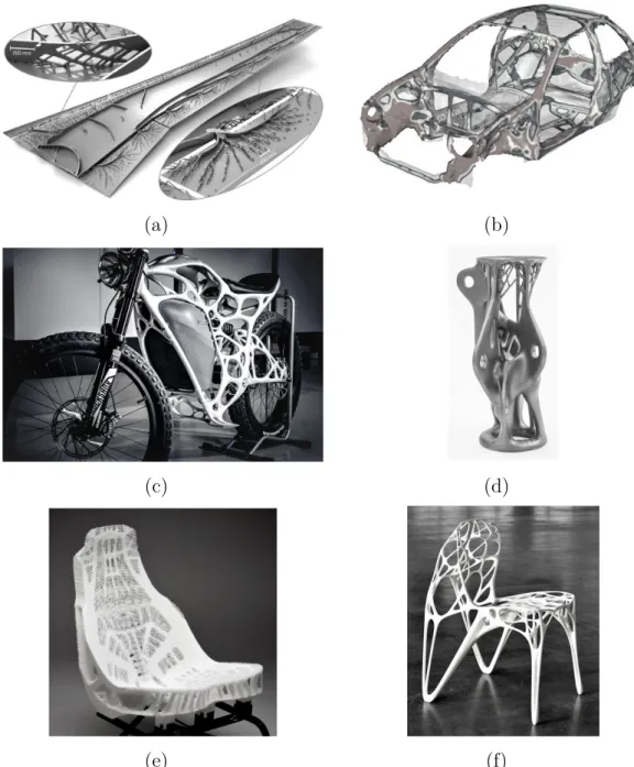
1.1 Example current state-of-the-art structures designed by topology opti-mization. (a) Concept aircraft wing (Technical University of Denmark); (b) automotive body structure (Altair Engineering); (c) motorcycle frame structure (Airbus APWorks); (d) structural steel component (Arup); (e) lightweight car seat prototype (Toyota Central R&D Labs); (f) Generico chair (Marco Hemmerling and Ulrich Nether). (Online images) . . . 3 1.2 A conventional chair assembly designed for economical production.

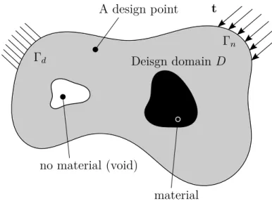
(On-line images) . . . 4 1.3 Conventional, single-piece continuum topology optimization problem

de-scription. . . 5 2.1 The non-gradient discrete framework for multi-component topology

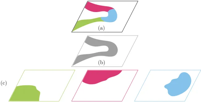
opti-mization. Different colors indicate different components. The thin black elements indicate joint locations. (a) Design domain; (b) discretized de-sign domain; (c) ground topology graph; (d) topology graph of a certain design; (e) realized multi-component design; (f) repaired multi-component design. . . 10 2.2 Demonstration of the two-layer design field, and the resulting simulation

model for an example case of number of components K = 3. (a) Simula-tion model; (b) density field ρ; (c) membership field m(k)_{. . . .} ₁₂

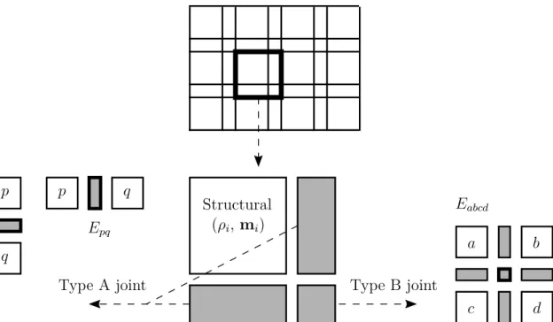
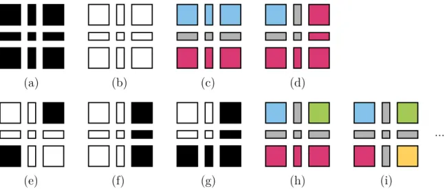
3.1 Definition of the design variables, structural element, and two joint ele-ment types. . . 16 3.2 Sample extreme scenarios for Type A joints. Black, gray and white colors

represent the structural materials, joint materials, and voids, respectively. Other colors represent different components with structural materials. (a) Between two, fully dense structural elements that belong to the same component; (b) between two, fully dense structural elements that belong to different components; (c) between two voids; and (d) between a fully dense structural element and a void. . . 17

(7)

3.3 Sample extreme scenarios for type B joints. Black, gray, and white colors represent the structural materials, joint materials, and voids, respectively. Other colors represent different components with structural materials. (a) Between four, fully dense structural elements that belong to the same component; (b) between four voids; (c-d) between four, fully dense struc-tural elements that belong to two different components; (e-f) between two, fully dense structural elements that belong to the same component and two voids; (g) between three, fully dense structural elements that be-long to the same component and one void; (h) between four, fully dense structural elements that belong to three different components; and (i) between four, fully dense structural elements that belong to four different components. . . 18 3.4 Computation of the bounding box with the continuously relaxed design

variables. This is a mesh-dependent formulation. (The mesh-independent formulation is presented in Figure 5.1.) . . . 21 3.5 Design domain and boundary condition settings for the (a) cantilever

example; (b) Messerschmidt-Bölkow-Blohm beam example. . . 24 3.6 Optimization iterative details for the cantilever example at (a) iteration

1; (b) iteration 5; (c) iteration 10; (d) iteration 15; (e) iteration 30; and (f) iteration 74. . . 26 3.7 A comparison between the multi-component topology and conventional,

single-piece topology for the cantilever example. (a) The optimized multi-component cantilever topology design. The gray regions indicate joint locations (assuming spot-welding joints) with the smaller Young’s mod-ulus than base structural materials; (b) the conventional, single-piece cantilever topology design. . . 27 3.8 Convergence history of the cantilever example. Due to the relatively

coarse mesh in this example, the complexity (die machining cost) con-straint was not included. . . 28 3.9 Multi-component topology designs of the Messerschmidt-Bölkow-Blohm

beam example with different levels of complexity control. (a) High die machining cost (complexity index: 3.99); (b) moderate die machining cost (complexity index: 3.45); (c) low die machining cost (complexity index: 3.03). From left to right: multi-component topology, “true” bounding box, and “true” perimeter. . . 29 4.1 A qualitative comparison of different composite manufacturing processes

in terms of the production cost in large quantities (vertical axis) and free-dom in orientation control (horizontal axis). As a manufacturing process becomes more economical for mass production, it sacrifices freedom in controlling fiber orientations. The suitability of different topology design methods is also plotted. (SFIM: short fiber injection molding; ATL: auto-mated tape layout; TFP: tailored fiber placement; CFP: continuous fiber printing) . . . 32

(8)

4.2 Demonstration of the three-layer design field and the resulting simula-tion model for an example case of number of components K = 3. (a) Simulation model; (b) density field ρ; (c) membership field m(k); (d) ori-entation field ϑ(k)_{. (The material orientation for each component can}

be either unidirectional or curvilinear based on the regularization filter radius used. This figure only shows the unidirectional case.) . . . 35 4.3 Coordinate transformation for the Cartesian orientation representation

through an isoparametric projection method. . . 37 4.4 Coordinate transformation for the component membership design field

through aK-dimensional cube-to-simplex projection for an example case

of K = 3. . . 38 4.5 The cube-to-simplex projection examples for cases of (a) K = 2 and (b)

K = 3. . . 39 4.6 Design domain and boundary conditions for the single load cantilever

problem. . . 44 4.7 Iterative details of all design fields for the single load cantilever problem

with K = 3 at (a) iteration 1; (b) iteration 5; (c) iteration 50; and (d) iteration 200. . . 45 4.8 Iterative details for the convergence of the component membership field

at (a) iteration 1; (b) iteration 5; (c) iteration 50; and (d) iteration 200. 47 4.9 The optimized three-component topology with component-wise

unidirec-tional orientations. Its optimized structural compliance is 6.21. . . 48 4.10 Convergence history for the single load cantilever problem with K = 3.

(a) Compliance (objective function); (b) volume constraint; (c) member-ship unity measure; (d) material anisotropicity constraints. (The mem-bership unity measure is plotted for the monitoring purpose, which is not included as a constraint in the optimization.) . . . 49 4.11 (a) Optimized single-piece topology with an isotropic material. Its

opti-mized structural compliance is 9.92; (b) optiopti-mized single-piece topology with continuous material orientation. Its optimized structural compliance is 4.07. . . 50 4.12 The optimized three-component design allowing component-wise

curvi-linear orientations. Its optimized structural compliance is 5.65. (a) The optimized multi-component topology; (b) the optimized density field ρ; (c) from left to right: the optimized membership fieldm(k)_{, the optimized}

component field (product of the two) ρm(k)_{, and the optimized material}

orientation field ϑ(k). . . 51 4.13 The optimized multi-component topologies with different number of

(9)

4.14 Design domain and boundary conditions for the multi-load tandem bicycle frame example, where t(xp) = −1.5; t(yp) = −1.0; t(xh) = 1.0; t(yh) = −1.0;

wx ={−1.0,−0.25}; and wy ={−6.0,−1.5}. At location (0.0,2.0), both

degrees of freedom inx andy are fixed. At location(63.5,16.0), only the degree of freedom inyis fixed. The lower left corner of the design domain is set as location(0.0,0.0). . . 53 4.15 (a) The optimized single-piece tandem bicycle frame structure with an

isotropic material; (b) the deformed structure under the heavy front load-ing condition; (c) the deformed structure under the heavy rear loadload-ing condition. Its optimized multi-load structural compliance is 4952. . . 54 4.16 The optimized multi-component tandem bicycle frame structure with

component-wise unidirectional material orientations. Its optimized multi-load structural compliance is 3312. (a) The optimized multi-component topology; (b) the optimized density fieldρ; (c) from left to right: the op-timized membership field m(k)_{, the optimized component field (product}

of the two) ρm(k)_{, and the orientation field}_ϑ(k)_{. . . .} ₅₅

5.1 Computation of the bounding box. This is a mesh-independent formula-tion. (The mesh-dependent formulation was presented in Figure 3.4.) . . 61 5.2 Problem description of multi-component topology optimization for

pow-der bed additive manufacturing. . . 64 5.3 Design domain and boundary condition settings for the (a)

Messerschmidt-Bölkow-Blohm beam example; (b) cantilever example. . . 67 5.4 Design field iterative details for the Messerschmidt-Bölkow-Blohm beam

example at (a) iteration 1; (b) iteration 35; (c) iteration 80; and (d) iteration 311. . . 69 5.5 Component interface explanation. The gray zone between component

boundaries is less stiff than regular base materials in the simulation model. Different colors indicate different components. . . 70 5.6 Manufacturing constraint iterative details for the

Messerschmidt-Bölkow-Blohm beam example at (a) Iteration 1; (b) iteration 35; (c) iteration 80; and (d) iteration 311. . . 71 5.7 The optimized multi-component topology for the MBB beam example.

The prescribed, maximum allowable build volume is plotted for each com-ponent. Different colors indicate different components. . . 72 5.8 The optimized topologies for the cantilever example with different

pre-scribed maximum allowable build volume: (a) 2.0×1.0; (b) 1.5×0.6; (c) 1.0×0.4; (d) 2.5×0.3; (e) the prescribed maximum allowable build volume for (a-d). . . 73 5.9 Design domain and boundary condition settings for the 3D simply-supported

center loading example. . . 74 5.10 The conventional, single-piece optimized topology for the 3D

simply-supported center loading example without applying manufacturing con-straints. (a) The quarter domain optimized structure; (b) the mirrored half domain structure. . . 75

(10)

5.11 The full domain optimized multi-component topology for the 3D simply-supported center loading example with manufacturing constraints. (a) The full domain optimized multi-component structure; (b) the sliced half domain multi-component structure. . . 76

(11)

LIST OF TABLES

4.1 Material properties for the numerical examples. . . 42 4.2 Summary of the structural performance and estimated mass-production

cost of cantilever designs discussed in Section 4.7.1. . . 52 5.1 Material properties and parameters for numerical examples. . . 66

(12)

LIST OF ABBREVIATIONS

ABB Axis-aligned Bounding Box ATL Automated Tape Layout BIW Body In White

BFGS Broyden–Fletcher–Goldfarb–Shanno CFP Continuous Fiber Printing

DMO Discrete Material Optimization ESO Evolutionary Structural Optimization

M3TO Multi-component Multi-material Multi-process Topology Optimization MABB Minimum Area Bounding Box

MBB Messerschmidt-Bölkow-Blohm

MTO Multi-component Topology Optimization

MTO-A Multi-component Topology Optimization for Additive manufacturing MTO-C Multi-component Topology Optimization for Composite manufacturing MTO-S Multi-component Topology Optimization for Stamping

OBB Oriented Bounding Box

SIMP Solid Isotropic Material with Penalization SFIM Short Fiber Injection Molding

TFP Tailored Fiber Placement VAC Variable Axial Composite

(13)

ABSTRACT

Topology optimization is a method where the distribution of materials within a design domain is optimized for a structural performance. Since the geometry is rep-resented non-parametrically, it facilitates innovative designs through the exploration of arbitrary shapes. Due to its unconstrained exploration, however, topology opti-mization often generates impractical designs with features that prevent economical manufacturing, e.g., complex perimeters and many holes. Above all, existing topol-ogy optimization methods assume that the optimized structure will be made as a single piece.

However, structures are usually not monolithic (i.e., single-piece), but assemblies of multiple components, e.g., cars, airplanes, or even chairs. It is mainly because pro-ducing multiple components with simple geometries is often less expensive (i.e., better manufacturability) than producing a large single-piece part with complex geometries, even with the additional cost of assembly.

This dissertation discussed a topology optimization method for designing struc-tures assembled from components, each built by a certain manufacturing process, termed the Multi-component Topology Optimization (MTO). The prior art of MTO used discrete formulations solved by genetic algorithms. To overcome the high com-putational cost associated with non-gradient heuristic optimization, this dissertation proposed a continuously relaxed gradient-based formulation for MTO. The proposed formulation was demonstrated with three manufacturing processes.

For the sheet metal stamping process, by modeling stamping die cost manufactur-ing constraints and assummanufactur-ing resistant spot weldmanufactur-ing joints, the simultaneous optimiza-tion of base topology and component decomposioptimiza-tion was, for the first time, attained using an efficient gradient-based optimization algorithm based on design sensitivities. For the composite manufacturing process, a cube-to-simplex projection and pe-nalization method was proposed to handle the membership unity requirement. With the multi-component concept, a unique structural design solution for economical com-posite manufacturing was achieved. The component-wise anisotropic material orien-tation design for topology optimization was presented without prescribing a set of alternative discrete angles as required by most existing material orientation methods.

(14)

For the additive manufacturing process, the MTO method enabled the design of additively manufactured structures larger than the printer’s build volume. By modeling manufacturing constraints on the build volume limit and elimination of enclosed holes, the optimized structure was an assembly of multiple components, each produced by a powder bed additive manufacturing machine. The first reported 3D example of MTO was presented.

(15)

CHAPTER 1

Introduction

1.1

Motivation

Structures are usually not monolithic (i.e., single-piece), but assemblies of multiple components. For example, a car usually has about 30000 parts [1]. The Boeing 737 airplane is made up of367000parts [2]. Most dinosaur skeletons have several hundred individual bones [3]. Even a frying pan is made of a disc base and a handle.

This dissertation was originally motivated by a fundamental question: why so many parts for structural products? Apparently, if different materials are necessary, a product has to be decomposed into pieces. This is the case for the frying pan, which requires thermal insulation materials to prevent the handle from getting too hot and heat conduction materials to heat up food. In addition, if relative motions are required, a structure also has to be decomposed into pieces. This is the case for dinosaur skeletons, where bones, connected by muscles and joints, move relative to each other.

However, the above two arguments are not applicable to the automotive Body In White (BIW), which is usually an assembly of many sheet metal stamped components joined by resistance spot welding. An automotive BIW can be made from a single material (e.g., steel), and does not involve any relative motions. It is mainly because producing multiple components with simple geometries are less expensive than pro-ducing a single piece BIW with complex geometries, even with the additional cost of assembly. In other words, the manufacturability of multi-component structures is often much better than that of single-piece structures. The manufacturability argu-ment for a multi-component structural product is the main motivation and focus of this dissertation while the other two, i.e., the materials and relative motions, are not.

(16)

1.2

Background

Topology optimization is a method for designing structures by optimally distributing materials within a prescribed design domain. It is an interdisciplinary research area between computational mechanics and design optimization. Unlike sizing and shape optimization, which are often based on parametric geometry representations, topology optimization describes geometries non-parametrically. It facilitates innovative designs through the exploration of arbitrary shapes.

Figure 1.1 presents several state-of-the-art example structures designed by topol-ogy optimization. It is obvious to see that structures generated by topoltopol-ogy op-timization are vastly different from conventional designs. Such out-of-box designs demonstrated the benefit of topology optimization in design exploration. However, these examples also revealed another significant shortcoming of designs generated by topology optimization: lack of manufacturability. Structures shown in Figure 1.1(a– b) are 3D digital models, which are still far away from realization into airplanes and cars. Structures shown in Figure 1.1(c–f) are prototypes produced by additive man-ufacturing, which are clearly not ready for economical production in large quantities. As seen in Figure 1.1, current state-of-the-art topology optimization designs share two major similarities, i.e., the complex overall geometry and the single-piece design, both of which lead to their lack of manufacturability. In contrast, structures de-signed for improved manufacturability or economical production in large quantities are usually assemblies of multiple components with simple component geometries. For example, Figure 1.2 shows a conventional chair assembly designed for economical production, which is composed of multiple beam and plate components assembled with fasteners.

The rest of this section reviews topology optimization methods (Section 1.2.1) and two related topics about improving manufacturability for topology optimization. Section 1.2.2 discusses related works in single-piece topology optimization for man-ufacturability. Section 1.2.3 discusses previous works in topology optimization of multi-component structures.

1.2.1

Topology optimization

According to [4], topology optimization is a natural outcome of introducing the mate-rial micro-structure design to shape and sizing optimization. Cheng & Olhoff (1981) discussed the optimal thickness distribution for elastic plates [5]. Their work led to a series of works on optimal design problems introducing micro-structure. Kikuchi

(17)

(a) (b)

(c) (d)

(e) (f)

Figure 1.1: Example current state-of-the-art structures designed by topology opti-mization. (a) Concept aircraft wing (Technical University of Denmark); (b) auto-motive body structure (Altair Engineering); (c) motorcycle frame structure (Airbus APWorks); (d) structural steel component (Arup); (e) lightweight car seat proto-type (Toyota Central R&D Labs); (f) Generico chair (Marco Hemmerling and Ulrich Nether). (Online images)

(18)

Figure 1.2: A conventional chair assembly designed for economical production. (On-line images)

and Bendsøe (1988) first introduced the material distribution approach for topology optimization [6].

Since the late 1980s, different methods have been developed for topology optimiza-tion, e.g., the Solid Isotropic Material with Penalization (SIMP) method [7, 8], the Evolutionary Structural Optimization (ESO) method [9], the topological derivative-based and level-set method [10, 11, 12, 13], the non-gradient method [14, 15], and the moving morphable components method [16]. For general introduction of dif-ferent topology optimization methods, readers are referred to several review pa-pers [17, 18, 19,20].

Based on different types of design domains, topology optimization can be classified into discrete (truss/beam) approaches and continuum (pixel/voxel) approaches. The continuum approach is the focus of this dissertation. Since the optimal structures of the discrete approaches are the collections of predefined primitive members, such as trusses and beams, the continuum approaches have advantages in representing realistic products with complex geometries.

Based on different types of optimization algorithms utilized, topology optimiza-tion can be classified into gradient-based methods and non-gradient methods. The gradient-based method is the focus of this dissertation. Recently, in topology opti-mization community, non-gradient methods received some serious critiques regarding their applicability in continuum topology optimization problems [18, 21]. It is due, mainly, to their lack of design sensitivities (i.e., gradient information), and the asso-ciated high computational cost.

(19)

optimiza-A design point material no material (void) Deisgn domain D Γn Γd t

Figure 1.3: Conventional, single-piece continuum topology optimization problem de-scription.

tion problem description. In a prescribed design domain D, under given boundary conditions (e.g., displacement boundary condition on Γd and traction boundary

con-dition on Γn), the problem is to optimize a structural performance by designing the

existence of materials in each design point, subject to some constraints (e.g., volume fraction). It can be summarized as a generalized shape design problem of finding the optimal material distribution.

Other than mechanical design problems, topology optimization has also been ap-plied to a variety of other applications, e.g., heat transfer [22], turbulent flow [23], antennas [24], architecture [25], and micro-systems [26].

1.2.2

Topology optimization for manufacturability

This section discusses manufacturing constraints for conventional, single-piece topol-ogy optimization. Two major classes are discussed including the general-purpose manufacturing constraints and process-specific manufacturing constraints.

It is well-known that continuum topology optimization tends to generate numer-ous small holes, i.e., checkerboards [27,28]. This behavior leads to mesh-dependency and non-existence of solutions. To resolve this issue, regularization schemes have been developed. They can be summarized into two main categories, the filtering methods [29, 30, 31, 32] and the constraint methods [33, 34, 28, 35, 36]. Recently, the PDE-based filtering method [37, 38] gained popularity due to its ease of imple-mentation and superior computational efficiency. When a regularization scheme is applied to topology optimization, it not only avoids numerical instabilities, but

(20)

gen-erates results with much simpler geometries. The reduced shape complexity usually leads to better general manufacturability. Therefore, such regularization schemes are regarded as general-purpose manufacturing constraints.

Manufacturing constraints modeled for certain manufacturing processes are re-ferred to as process-specific manufacturing constraints. Such constraints are usually imposed on part geometries. They are often more specific than general-purpose man-ufacturing constraints. For example, if a part is designed for molding and casting, it has to be open and lined up with the draw direction of the die. If this restric-tion is not applied to topology optimizarestric-tion, the resulting geometry is likely to have cavities and overhang features that would prohibit drawing the die. To ensure the manufacturability of structural topology designs for molding and casting, Zhou et al. (2002) [39] proposed to model the moldability constraint as additional single variable linear inequality constraints. Similar moldability manufacturing constraints were in-tegrated into level-set topology optimization [40, 41]. Recently, methods based on fictitious physical models were developed to ensure the moldability of topology opti-mized structures [42, 43]. Extrusion constraints have also been proposed to enforce uniform cross-sections [39,44]. To better conform to manufacturing processes tailored to plate structures, a geometry projection method was proposed to generate assem-blies of discrete geometric components [45,46]. For composite resin transfer molding, a data-driven model for resin filling time prediction was developed and integrated into topology optimization [47]. To reduce the amount of support materials required for additive manufacturing, different overhang manufacturing constraint methods were developed (e.g., [48, 49, 50, 51, 52, 53, 54]). For parts designed for additive man-ufacturing, enclosed voids should be avoided, so that the un-melted metal powders or internal support materials can be removed from the component once it has been built. A virtual temperature method was proposed to eliminate enclosed voids by constraining the maximum temperature field of a fictitious thermal analysis [55, 56]. To generate bone-like porous structures as lightweight infill for additive manufactur-ing, the method based on an upper bound constraint on localized material volume fraction was proposed [57, 58].

For more manufacturing oriented topology optimization methods, readers are re-ferred to recent review papers [59,60].

In summary, while the integration of manufacturing constraints in topology opti-mization can lead to better manufacturability of the optimized structure, its perfor-mance is often degraded. In some cases, the sacrifice of structural perforperfor-mance can be drastic. It is partially because the manufacturing constraints are always applied

(21)

to the entire single-piece structure. The single-piece assumption may overly simplify the geometries, which goes completely against the benefit of topology optimization. However, in the scope of this dissertation, when manufacturing constraints are ap-plied to each individual component of a multi-component structure instead of the entire single-piece structure, they will gain new interpretations.

1.2.3 Multi-component topology optimization

MTO is an evolution of conventional, monolithic (i.e., single-piece) topology opti-mization, which not only optimizes the overall base topology, but the component decomposition. From a viewpoint of mathematical formulation, it is closely related to multi-material topology optimization (e.g., [61, 62, 63, 64, 65, 66]), where differ-ent materials in multi-material structures can be regarded as differdiffer-ent compondiffer-ents in multi-component structures. Unlike most topology optimization studies (includ-ing multi-material topology optimization) that focus merely on optimiz(includ-ing various structural performances, MTO is motivated by the need of generating ready-to-manufacture optimal structures made as assemblies of multiple components, each of which conforms geometric constraints imposed by a chosen manufacturing process. Another related topic to MTO is the topology optimization for embedded compo-nents, also known as the component layout optimization (e.g., [67, 68, 69, 70, 71, 72,

73]). Though these works are important for certain applications, e.g., the integration of rigid objects, actuators and integrated circuits, the components are assumed with fixed geometries and only allowed floating during the course of optimization.

There are three major classes in prior art of MTO. The first class assumes a priori knowledge of joint locations [74, 75, 76, 77]. The second class assumes that component decomposition is an independent problem from base topology optimiza-tion [78, 79, 80, 81, 82]. By relaxing the above two assumptions, the third class poses the simultaneous optimization of base topology and component decomposi-tion, which is the focus of this dissertation. It was originally formulated as discrete optimization problems and solved by genetic algorithms [83, 84, 85]. However, as discussed in Section 1.2.1, such non-gradient heuristic methods for topology opti-mization have received criticisms regarding their computational inefficiency for high resolution problems [18, 21]. To address the criticisms, this dissertation proposes to model the component decomposition as a relaxed continuous problem, and developed a gradient-based framework for MTO.

(22)

MTO can be directly applied to designing structures assembled from components, each built by a certain manufacturing process.

1.3

Dissertation goal

The primary goal of this dissertation is to develop a new mathematical formulation for MTO that can provide scalable multi-component structural design solutions, which also take manufacturing limitations into account. Prior MTO methods were limited to discrete formulations solved by genetic algorithms, which were not suitable for large-scale problems.

The secondary goal is to expand MTO applications to varieties of manufacturing processes. Prior MTO methods were limited to the sheet metal stamping process.

1.4

Dissertation outline

The remainder of this dissertation is organized as follows. Chapter 2 presents a gen-eral gradient-based continuous framework for MTO. Chapter 3, 4, and 5 discuss three MTO applications, including stamping, composite manufacturing, and addi-tive manufacturing. Finally, Chapter 6 summarizes the dissertation and discusses opportunities for future research.

(23)

CHAPTER 2

A general gradient-based continuous formulation for

multi-component topology optimization

This chapter introduces a new gradient-based continuous framework for MTO. It is a relaxation of the discrete formulation in [84] and [85], which is briefly reviewed first in Section 2.1 for the sake of comparison.

2.1

Prior art: non-gradient discrete formulation

As seen in Figure 2.1(b), a prescribed design domain D is discretized into finite elements such that every other adjacent structural element (square) sandwiches a joint element (thin rectangle). Discrete design variables are assigned to both structural (x) and joint (y) elements, where:

xi =   

1 if structural material exists in element i

0 otherwise , and yj =         

2 if joint material exists in element j 1 if structural material exists in element j 0 otherwise

.

In the case ofyj = 2, it indicates the existing of a joint in elementj, and the neighbor

two structural elements belonging to different components.

Figure 2.1(c) shows a ground topology graph such that a node represents a struc-tural element, and an edge represents a joint element. A given combination ofx and

y can be interpreted as a unique topology graph, e.g., Figure 2.1(d). After certain repairing of invalid structures, a topology graph is realized as a multi-component

(24)

Design domain D

(a) (b) (c)

(d) (e) (f)

Figure 2.1: The non-gradient discrete framework for multi-component topology op-timization. Different colors indicate different components. The thin black elements indicate joint locations. (a) Design domain; (b) discretized design domain; (c) ground topology graph; (d) topology graph of a certain design; (e) realized multi-component design; (f) repaired multi-component design.

(25)

topology design, e.g., Figure 2.1(f).

Using discrete variables x and y, a multi-objective MTO problem can be formu-lated with both structural performance and manufacturing costs modeled as objec-tives. Additional constraints can be added if needed, e.g., weight target. Because the overall optimization problem is modeled with discrete variables and manufacturing cost functions are often not directly differentiable, in [84], a multi-objective genetic algorithm was used to solve it.

As discussed in Chapter 1, such non-gradient discrete formulation will encounter computational efficiency limitations. With the Kriging-interpolated level-set exten-sion [85], the number of design variables can be significantly reduced. However, due to the nature of non-gradient methods and lack of sensitivity information during optimization, the computational efficiency improvement is still marginal.

To overcome these challenges, this dissertation presents a continuously relaxed formulation for MTO in a gradient-based framework. For the first time, the simulta-neous optimization of base topology and component decomposition is attained using an efficient gradient-based optimization algorithm based on design sensitivities.

2.2

Continuously relaxed design field

As demonstrated in Figure 2.2, in the continuous MTO formulation, there are two layers of design fields. The first layer is the material density fieldρ as a common field for all components, which describes the overall base topology. The second layer is the membership vector field m = (m(1)_{, m}(2)_,· · · _{, m}(K)₎_. _m(k) _{represents the fractional}

membership of a design point in the design domain to the k-th component, k = 1,2,· · · , K, where K is the prescribed, maximum allowable number of components. The specification ofKis not needed in the discrete formulation as discussed in Section 2.1. Both ρ and m(k) are continuous variables ranging between 0 and 1. In order to ensure the unique selection of the component for each design point, an additional important criterion needs to be satisfied at the end of optimization. The membership to only one component converges to 1 while the memberships to all other components converge to 0. In this dissertation, different methods have been proposed to meet this requirement. Chapter 3 proposes to use many equality constraints to ensure the unity of fractional component memberships. For each design point i, a linear constraint

∑K k=1m

(k)

i = 1 is added. In Chapter 4 and 5, different nonlinear projection methods

(26)

(a)

(b)

(c)

Figure 2.2: Demonstration of the two-layer design field, and the resulting simulation model for an example case of number of components K = 3. (a) Simulation model; (b) density field ρ; (c) membership field m(k)_.

2.3

Continuously relaxed formulation

With the continuously relaxed design field, a general gradient-based continuous MTO formulation can be summarized as follows:

minimize ρ,m(1)_,_···_,m(K) F subject to h≤0 ρ∈[0,1]D for k = 1,2,· · ·, K : g(k) ≤0 m(k) ∈[0,1]D , (2.1)

where ρ and m(k) are the density and membership design fields; F is the structural performance objective (e.g., stiffness and strength); g(k) _{is a vector of manufacturing}

constraints applied to each decomposed component k based on different manufac-turing process applications; h is a vector of other constraints based on other design requirements (e.g., volume fraction). Both the objective (F) and constraints (h and

g(k)_{) should be modeled as continuous and differentiable functions with respect to all}

(27)

The manufacturing constraint modeling for gradient-based topology optimization has been a challenging task due to the nature of “blurry” intermediate topologies. Relaxation and approximation are often needed. For example, [28] used the total variation of the density field to approximate the complexity of an intermediate topol-ogy when its perimeter cannot be directly quantified. The MTO adds an additional layer of difficulties to the manufacturing constraint modeling, because the “blurry” effect is also applicable to the intermediate component decomposition. The compo-nent boundaries will not be clear until the end of optimization while the geometric constraint evaluation has to be done at the component level throughout the optimiza-tion.

2.4

Chapter summary

This chapter presented a general gradient-based continuous MTO formulation that will be used for different manufacturing processes in the rest of this dissertation. The overall base topology was described with a density design field following the conventional, density-based topology optimization methods (e.g., SIMP). To model the component decomposition in a relaxed continuous manner, the concept of frac-tional membership of a design point to different components was introduced. After the relaxation of design fields, the gradient-based continuous MTO formulation was presented, which built a foundation for the rest of this dissertation.

(28)

CHAPTER 3

Multi-component topology optimization for

stamping

This Chapter presents the MTO application to stamped sheet metal structures, termed the Multi-component Topology Optimization for Stamping (MTO-S). Stamp-ing is the process of placStamp-ing flat sheet metal into a stampStamp-ing die where a tool and the die surface will form the flat sheet metal into a net shape. Stamping has been widely used across different industries due to its primary advantage of high production rate with minimum operator intervention. As discussed in Chapter 1, most structural products are assemblies of multiple components. This is especially true for stamped sheet metal products. Different welding processes have been developed to connect the components into a final product assembly. While some products with small scale and simple geometries can be made as a single piece, e.g., water sinks, most sheet metal products are designed as multi-component structures, e.g., automotive, ships.

3.1

Why multiple components for stamped sheet metal

struc-tures

The cost of stamping dies contributes to the majority of the cost for manufacturing sheet metal products, which consists of the cost of die-set materials and the cost for machining the die. As die-set raw materials are usually purchased as rectangular prisms, the cost of die-set materials can be empirically modeled as proportional to the size of the bounding box enclosing each component [86]. The cost for machining the die can be modeled as proportional to a complexity index, which is defined as the perimeter of each component normalized by its bounding box size [86].

The sheet metal assemblies are usually joined by a welding process, which will inevitably require additional assembly costs compared with a single-piece product.

(29)

However, compared with the investment in stamping dies, the assembly cost is rela-tively low and sometimes even negligible.

Therefore, for a complex sheet metal product, it is often more cost effective to de-sign it as an assembly of multiple components with simple component geometries than producing a single-piece product with complex geometries, even with the additional cost of assembly.

The standard practice of designing a multi-component stamped sheet metal prod-uct is to design and optimize its overall (single-piece) base geometry first, and then decompose it to refine part boundaries and joint configurations. Such practice, known as a two-step approach, is likely to yield suboptimal solutions with respect to the overall structural performance and/or manufacturing and assembly costs, since the optimal decomposition obtained in the second step is largely dependent on the op-timal overall geometry obtained in the first step. The MTO-S method proposed in this chapter intends to realize the simultaneous design of the base topology and component decomposition for stamped sheet metal multi-component structures.

3.2

Domain discretization and design variable configuration

A prescribed design domain D is discretized into finite elements in the same man-ner as in Figure 2.1(b). Due to this special domain discretization, the mathematical formulation presented in this Chapter is mesh-dependent. Mesh-independent formu-lations will be presented in Chapter 4 and 5. Design variables are only defined in structural elements as shown in Figure 3.1. Following the two-layer design variables. For a structural element i, the (fictitious) densityρi takes a continuous value ranging

from zero to one, similar to the conventional SIMP formulation. The membership design variablemi is a vector of size K, where K is the prescribed, maximum

allow-able number of components. Each element m(_ik) of mi also takes a continuous value

ranging from zero to one, representing the fractional membership of elementiin com-ponent k. An additional linear constraint ∑K

k=1m (k)

i = 1is added to each structural

elementi in order to ensure the unity of total fractional memberships. Similar math-ematical formulations can be found in multi-material topology optimization studies (e.g., [87, 88]).

(30)

Structural (ρi, mi)

Type A joint Type B joint

p Epq Eabcd q p q a b c d

Figure 3.1: Definition of the design variables, structural element, and two joint ele-ment types.

3.3

Continuously-relaxed mesh-dependent joint model

The joint model assumes resistance spot-welding joints, which usually have less stiff-ness than structural members [89]. The joint model formulation, however, is general enough to be applicable to other joining processes with different material properties. There are two types of joint elements, as shown in Figure 3.1. One is the thin strip between two structural elementspandq, denoted as the Type A joint. The equivalent Young’s modulus of such joint elements is determined by density ρ and membership

m of the two neighbor structural elements. A joint stiffness matrix H is defined as a K ×K symmetric matrix where all diagonal elements are Young’s modulus of structural materials E(S), and all off-diagonal elements are Young’s modulus of joint materials E(J) (< E(S) for resistance spot-welded joints). Matrix H can be written as: H={hij}=    E(S) if i=j E(J) _if _i_̸₌_j . (3.1)

The equivalent Young’s modulus Epq of a Type A joint element between structural

elements pand q is computed as:

(31)

(a) (b) (c) (d) Figure 3.2: Sample extreme scenarios for Type A joints. Black, gray and white colors represent the structural materials, joint materials, and voids, respectively. Other colors represent different components with structural materials. (a) Between two, fully dense structural elements that belong to the same component; (b) between two, fully dense structural elements that belong to different components; (c) between two voids; and (d) between a fully dense structural element and a void.

whereρp andρq are densities of structural elementspandq, andmp andmq are their

corresponding memberships. Figure 3.2 shows sample extreme scenarios for Type A joints. The equivalent Young’s modulus of a Type A joint takes a value Epq = E(S)

if structural elements pand q both belong to the same component and have full den-sity values, indicating the joint element is actually a part of a structural member (Figure 3.2(a)); Epq = E(J) if the neighbor structural elements belong to different

components and have full density values, indicating the joint element represents a welded joint (Figure 3.2(b)); and Epq = 0 if at least one of p and q has zero density

value (Figure 3.2(c–d)). Otherwise, Epq takes a value between zero and E(S),

indi-cating the joint element is “in a fractional state”, somewhere between void (no weld) and structural solid.

The other type of joint element is the smaller square diagonal element, denoted as Type B joint in Figure 3.1. Its equivalent Young’s modulus Eabcd surrounded by

structural elements a, b, c, and d, is defined as the penalized average of the four neighbor Type A joint elements:

Eabcd = ((Eab+Eac+Ebd+Ecd)/4)Pw, (3.3)

where Eab, Eac, Ebd, and Ecd are the equivalent Young’s moduli of Type A joint

elements between structural elements a and b,a and c,b and d, and cand d,

respec-tively. The powerPw =log(E(S)₊_E(J)₎_/₂E(J) ensures thatE_abcd takes reasonable values

for most conceivable circumstances.

Figure 3.3 shows sample extreme scenarios for Type B joint elements. While the penalization strategy in Equation (3.3) is tuned to cover the most common scenarios in Figure 3.3(a–d), it produces somewhat (albeit negligibly infrequent) unnatural out-comes under several other scenarios such as the ones shown in Figure 3.3(e–i). Under the scenario in Figure 3.3(e), Equation (3.3) setsEabcd = 0, leading to a disconnected

(32)

(a) (b) (c) (d)

(e) (f) (g) (h) (i)

...

Figure 3.3: Sample extreme scenarios for type B joints. Black, gray, and white colors represent the structural materials, joint materials, and voids, respectively. Other colors represent different components with structural materials. (a) Between four, fully dense structural elements that belong to the same component; (b) between four voids; (c-d) between four, fully dense structural elements that belong to two different components; (e-f) between two, fully dense structural elements that belong to the same component and two voids; (g) between three, fully dense structural elements that belong to the same component and one void; (h) between four, fully dense structural elements that belong to three different components; and (i) between four, fully dense structural elements that belong to four different components.

component. However, this would be discouraged during the process of minimizing compliance, and also would potentially contribute to eliminating checkerboard pat-terns. Under the scenarios in Figure 3.3(f–g), Equation (3.3) assigns Eabcd with a

very small value that can be virtually considered as zero. The values of Eabcd in

conditions Figure 3.3(h–i) would be slightly smaller than E(J)_{. Since such conditions}

rarely happen, the effect would also be negligible.

3.4

Structural compliance objective considering the joint

prop-erty

As a result of the special domain discretization and the relaxed joint stiffness model discussed above, joint locations and properties can now be integrated into the overall structural compliance computation, written as:

(33)

where f is the external load and u is the solved displacement. K(E) is the global stiffness matrix assembled from the element stiffness Ke_. _K(E) _{is a function of}

E containing the equivalent Young’s moduli of structural and joint elements. For structural element i, the equivalent Young’s modulus Ei = ρPidE(S), which is the

power law in the conventional SIMP formulation. Pdis the density penalty parameter.

For joint elements, the equivalent Young’s moduli are calculated based on Equations (3.2) and (3.3).

3.5

Manufacturing constraint modeling for stamping

As discussed in Section 3.1, the manufacturing cost of a stamping die mainly consists of the die-set material cost and the cost for machining the die [86].

3.5.1 Die-set material cost

The cost of die-set materials is modeled as proportional to the area of the bounding box enclosing each component [86].

The computation of bounding boxes is a fundamental problem in computer graph-ics. Based on the tightness of the bounding box, it can be computed in several dif-ferent ways. The Axis-aligned Bounding Box (ABB) can be computed efficiently by fixing the orientation of the bounding box. However, it’s not sufficiently tight for many applications. The Oriented Bounding Box (OBB) whose orientation is deter-mined by an approximation analysis is much tighter than ABB yet still not optimal. The Minimum Area Bounding Box (MABB) is the theoretically ideal solution to de-scribe the size of a component. Unfortunately, its high computational complexity make it virtually unusable for practical problems. OBB is used in this dissertation to quantify the component size.

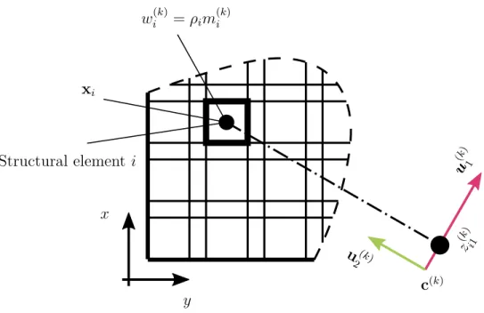
Many algorithms have been developed for the bounding box computation in com-puter graphics (e.g., [90, 91, 92, 93]). Unfortunately, existing algorithms are not directly applicable to our problem because they all require fixed input geometries with “clear” part boundaries. To accommodate the “blurry” intermediate topologies during the course of MTO, a weighted principal component analysis is proposed to approximate the orientation of the bounding box. A weighted projection method is proposed to approximate the size of the bounding box. The weighting function contains the information of both density and membership design variables. The den-sity design variables model the “blurry” effect on the overall base topology while the

(34)

membership design variables model the “blurry” effect regarding the intermediate component decomposition.

The orientation of the bounding box of component k is approximated using a weighted principal component analysis, where centroid xi of each structural element

i in the design domain is associated with a fictitious weight ρim

(k)

i as illustrated in

Figure 3.4. For each componentk, the weighted covariance matrixΣ(k)_{can be written}

as follows: Σ(k) = ∑N i=1ρim (k) i (xi)(xi)| ∑N i=1ρim (k) i , (3.5)

whereN is the number of structural elements. By applying the singular value decom-position onΣ(k)_{, two orthogonal principal components}_v(k)

1 andv (k)

2 can be extracted,

which will describe the approximate orientation of the OBB of component k.

The area of OBB of component k is approximated using the weighted projection variance, where the variances of the centroidsxi, weighted withρim

(k)

i , and projected

ontov(₁k) and v(₂k), are considered as the approximation of the length of the two sizes of the OBB. For each component k, the length (or width) of the OBB in direction

v(_jk) is approximated as a weighted projection variance:

l_j(k)= ∑N i=1ρim (k) i (z (k) ij −c (k) j )2 ∑N i=1ρim (k) i , (3.6)

where z_ij(k) = (xi)|vj(k) is the projection of xi onto v(jk), and c

(k)

j is the center of

component k in the v(_jk) direction, given as:

c(_jk) = ∑N i=1ρim (k) i z (k) ij ∑N i=1ρim (k) i . (3.7)

By multiplying the length and width, the area of the OBB for component k can be calculated, which is used as an approximation of the cost of die-set materials:

A(k) =

2

∏ j=1

(35)

x y w(_ik) =ρim (k) i Structural element i xi z (k) i1 u(_k₎ 2 u (k) 1 c(k)

Figure 3.4: Computation of the bounding box with the continuously relaxed design variables. This is a mesh-dependent formulation. (The mesh-independent formulation is presented in Figure 5.1.)

(36)

3.5.2

Die machining cost

The die machining cost for component k is modeled as proportional to a complexity index, which is the perimeter of each component normalized by its OBB size [86]:

X(k) = P

(k)

√

A(k), (3.9)

where P(k) is the perimeter length to be sheared during stamping. By generalizing the perimeter calculation, previously developed for single-piece topology optimiza-tion [28], P(k) _{can be approximated as the total variation of the density design}

vari-ables, weighted with the membership design varivari-ables, in a matrix form:

P(k) = nely∑−1 i=1 nelx ∑ j=1 |m(_ijk)ρij−m (k) i+1,jρi+1,j|+ nely ∑ i=1 nelx∑−1 j=1 |m(_ijk)ρij −m (k) i,j+1ρi,j+1|, (3.10)

where nelx and nely are the number of structural elements in x- and y-axis in the design domain. Due to the need of differentiability with respect to ρi and mi, the

absolute operator in Equation (3.10) is numerically approximated as:

|x| ≡√(1 + 2ε)x2₊_ε2−_ε, _(3.11)

whereεis a small positive real number balancing the accuracy and smoothness of the approximation.

It is noted that the manufacturing cost models discussed in this section would not be in the dollar-to-dollar level accuracy. It is due, mainly, to the numerical approxi-mations involved and other unknown factors, such as machine specifications and labor costs. However, in the concept generation stage, for which topology optimization is most suitable, the proposed simplified manufacturing cost models would be adequate for capturing the trend of manufacturing costs.

3.6

Optimization formulation

The overall MTO-S problem is formulated as the minimization of structural com-pliance subject to constraints on the cost of die-set materials and die machining,

(37)

summarized as follows: minimize ρ,m(1)_,_···_,_m(K) F(u) subject to g1 := K ∑ k=1 A(k)(ρ,m(k))≤α∗ g2 := K ∑ k=1 P(k)(_ρ_,_m(k)) √ A(k)(_ρ_,_m(k)) ≤β∗ for i= 1,2, ..., N : ρi ∈[0,1] g₃(i) := K ∑ k=1 m(_ik)= 1 for k = 1,2, ..., K and i= 1,2, ..., N : m(_ik) ∈[0,1] , (3.12)

where ρ and m(k) _{are the density and membership design variables;} _K _{is the}

pre-scribed, maximum allowable number of components; N is the number of structural elements; F is the structural compliance objective defined in Equation 3.4; A(k) _is

the approximate OBB area of component k; α∗ is the maximum allowable total OBB area (≈ die-set material cost); P(k) _{is the approximate perimeter of component} _k_;

and β∗ is the maximum allowable total complexity (≈die machining cost). The tra-ditional volume fraction constraint for topology optimization is not included, because the OBB area constraint serves a similar role as the volume fraction constraint. The additional constraint on memberships for each element i ensures the unity of the to-tal fractional memberships. Finally, both densities and memberships take continuous values ranging from zero to one.

3.7

Numerical results

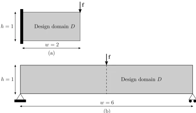
This section presents numerical results of the gradient-based MTO-S. A cantilever example is presented in Section 3.7.1 to show its detailed optimization iterations. Another Messerschmidt-Bölkow-Blohm (MBB) beam example is presented in Sec-tion 3.7.2 to demonstrate the effect of the die machining cost constraint. Their design domains and boundary conditions are summarized in Figure 3.5. Symmetry

(38)

bound-Design domainD w= 2 Design domain D f w= 6 h= 1 (b) (a) f h= 1 w= 2

Figure 3.5: Design domain and boundary condition settings for the (a) cantilever example; (b) Messerschmidt-Bölkow-Blohm beam example.

ary conditions were applied to the MBB example. The ratio of the width of Type A joint elements to the length of structural elements was set as 0.2 for the cantilever example. For problems with finer mesh, which was the case for the MBB example, this ratio was set to 1. The ratio of the Young’s modulus of joint elements to that of structural elements was set as 0.2, reflecting that spot-welding joints are less stiff than base structures. This value can also be set differently per design requirements. The convergence criteria for optimization are set as follows. The lower bounds on the size of a step and on the change in the value of the objective function were all set as

1e−5. The maximum number of iterations was set as 100 and 400 for the cantilever and MBB examples, respectively. The optimizer would terminate when any of the above three criteria was met.

The constrained optimization problem in Equation (3.12) was solved by the interior-point method using the Matlab fmincon. the first derivatives of the objective and con-straints were analytically derived with the assistance of the Matlab symbolic math toolbox, whereas the Hessian was numerically approximated using a finite-difference approach. The optimization usually converges within a few hundreds of iterations. For comparison, to solve similarly sized problems, previous methods based on non-gradient discrete formulations and genetic algorithms required significantly more func-tion evaluafunc-tions, e.g.,100000 in [84], and 60000in [85].

(39)

The finite-difference approximation of Hessian inevitably brings computational ef-ficiency concerns for large-scale studies. More computationally efficient implementa-tions can be achieved by, e.g., using the Broyden–Fletcher–Goldfarb–Shanno (BFGS) method to return a quasi-Newton approximation to the Hessian, deriving the Hessian analytically, and using first-order optimization solvers that do not require Hessian. In the past attempts by the authors, the BFGS required more iterations for convergence, likely due to its relatively inaccurate approximation compared with finite-differencing. Also, the algorithms that require only the first-order gradients did not perform well, due to the large number of linear equality constraints for membership unity.

3.7.1 Iterative details: cantilever

The proposed gradient-based continuous MTO-S is first applied to a10×5(structural element mesh) cantilever example to show its detailed optimization iterations. Its design domain D and boundary condition settings are presented in Figure 3.5(a).

The number of components was set asK = 3. As seen in Figure 3.6, at iteration 1, density and membership design variables ρi and m

(k)

i were uniformly initialized

as 0.4 and 1/K respectively. Due to the relatively coarse mesh in this example, the complexity (die machining cost) constraint was not included.

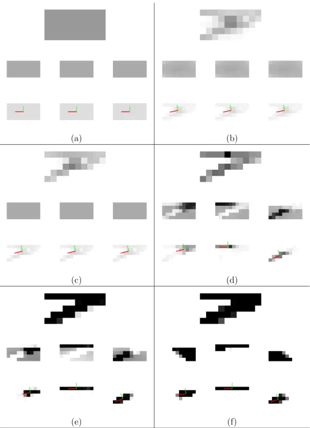
Figure 3.6 shows the iterative history of the density design variable ρi in the first

row, membership design variablem(_ik)in the second row, and intermediate components (product of the two) ρim(ik) in the third row. The red and green lines indicate the

orientation of bounding boxes. It can be seen that centers of the bounding boxes also update during optimization. As seen from the iterative details, membership variable

m(_ik) started to converge to a certain component at iteration 15. At the end of optimization, component boundaries were almost black and white when optimization converged at iteration 74.

Though several elements near the component boundaries still had fractional mem-berships, they were resolved by assigning those elements to the component with the largest m(_ik). The post-processed multi-component topology design is shown in Fig-ure 3.7(a). The thin gray elements between every two components are the resulting joint locations with the less stiff Young’s modulus. For a comparison, the optimized single-piece topology design using the conventional SIMP approach without regular-ization is presented in Fig. 3.7(b). Even without the complexity constraint that would penalize checkerboard patterns, they did not appear in the result in Fig. 3.7(a). It appears that the combination of having no volume constraint and the introduction

(40)

(a) (b)

(c) (d)

(e) (f)

Figure 3.6: Optimization iterative details for the cantilever example at (a) iteration 1; (b) iteration 5; (c) iteration 10; (d) iteration 15; (e) iteration 30; and (f) iteration 74.

(41)

(a) (b)

Figure 3.7: A comparison between the multi-component topology and conventional, single-piece topology for the cantilever example. (a) The optimized multi-component cantilever topology design. The gray regions indicate joint locations (assuming spot-welding joints) with the smaller Young’s modulus than base structural materials; (b) the conventional, single-piece cantilever topology design.

of the total bounding box area constraint encourages designs without checkerboard in order to have more materials. The special domain discretization also contributes to the elimination of checkerboard patterns in the optimized topology.

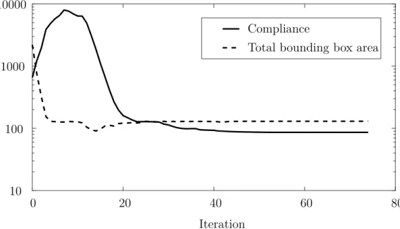
Figure 3.8 presents the optimization convergence history. Since the total bound-ing box area constraint was violated initially, the optimizer attempted to decrease the total bounding box area in early iterations while sacrificing the compliance ob-jective. Once the total bounding box area constraint reached the prescribed limit α∗, the optimizer continued by minimizing the compliance objective, driven mainly by the compliance sensitivity while keeping the manufacturing constraint active. The optimization converged in 74 iterations when the termination criterion for the change of objective value was met.

3.7.2

Die machining cost: Messerschmidt-Bölkow-Blohm beam

This section discusses the effects of the complexity (i.e., die machining cost) con-straint limit β∗ through a 240×40MBB example. Its design domain and boundary condition settings are shown in Figure 3.5(b). Only half of the design domain was optimized because of the symmetry in boundary conditions and the initial design do-main. While checkerboard patterns were discouraged by the new total bounding box area constraint and the special domain discretization, undesired small features would still appear for problems with increased mesh, which in turn would increase the die machining cost. Therefore, a complexity constraint, as described in Equation (3.9),

(42)

0 20 40 60 80 10 100 1000 10000 Compliance

Total bounding box area

Iteration

Figure 3.8: Convergence history of the cantilever example. Due to the relatively coarse mesh in this example, the complexity (die machining cost) constraint was not included.

was introduced to control the die machining cost.

Figure 3.9 shows three multi-component topology designs with different settings of the complexity constraint limitβ∗. The same value of the total bounding box area constraint limit α∗ was applied to all three cases. Figure 3.9 also presents the “true” bounding box and “true” perimeter for each decomposed component. Lower com-plexity indices 3.45 and 3.03 were achieved by decreasing the comcom-plexity constraint limit β∗ compared with the baseline 3.99 with the limit β∗ =∞ (i.e., no complexity control). Once again, even without the complexity control, checkerboard patterns did not appear, as seen in Figure 3.9(a). With the decrease of β∗, the overall com-plexity of the optimized topology could be reduced, resulting in less expensive overall stamping die machining cost. Similar effect on the complexity control could also be achieved by filtering methods. It was observed that the complexity constraint limit

β∗ had little influence on the component decomposition, but greater effect on the overall base topology of the multi-component structures.

3.8

Chapter summary

This chapter proposed a topology optimization method for structures made of sheet metal components. With the continuous density and membership design variables and the cost modeling of stamping dies, simultaneous optimization of the overall

(43)

(a)

(b)

(c)

Figure 3.9: Multi-component topology designs of the Messerschmidt-Bölkow-Blohm beam example with different levels of complexity control. (a) High die machining cost (complexity index: 3.99); (b) moderate die machining cost (complexity index: 3.45); (c) low die machining cost (complexity index: 3.03). From left to right: multi-component topology, “true” bounding box, and “true” perimeter.

(44)

base topology and component decomposition was realized in a continuously relaxed manner. A continuously relaxed joint stiffness model was also developed to con-sider the component interface property in the structural performance analysis. The simplified cost model for stamping dies was developed based on an empirical cost model [86]. As a result, MTO was, for the first time, solved using a gradient-based method, which demonstrated promising potentials to dramatically improve the com-putational efficiency over previous discrete formulations solved by genetic algorithms (e.g., [84, 85]).

However, the development of the gradient-based MTO method was still in its in-fancy. Some major limitations of MTO-S are acknowledged as follows. Though the complexity control can help generate mesh-independent results without checkerboard patterns, due to the special domain discretization and mesh-dependent joint stiffness modeling, the overall MTO-S formulation is still deemed mesh-dependent. More-over, to ensure the membership unity for each structural element, a large number of equality constraints are required in the MTO-S formulation. Equality constraints are generally not favored by gradient-based optimization, especially with large quanti-ties. Therefore, the MTO-S problem was solved with the need of Hessian calculat