1Abstract—In this paper we present a new method to obtain the density of solid composites using ultrasound. The method exploits the relation between density and acoustic impedance and only requires the measurement of a reference signal form the interface water-air. Once made in a controlled environment, it can be used for any material, and does not require any additional measurement or set-up, so that with a simple calculus it can be used with automatic ultrasonic measurements to calculate the density and therefore elastic constants of the composite for its complete characterization. The method is applied to 3 different materials: two composites based on epoxy and polyester resins respectively with unknown final properties and a common methacrylate sample used as reference. Results show good concordance between obtained and expected results.
Index Terms—Ultrasound; composite; material characteri-zation; density.
I. INTRODUCTION
Composite materials are nowadays a key component in most of the industries developments and can be found in almost any product, from the most advanced satellite to the carcass that protects our smart mobile. In recent years it has become widespread starting to use nanoparticles of different materials (such as carbon or graphene nanoparticles) to modify the properties of the composites. Given the novelty of the introduction of these materials in commercial products and the difficulty of their integration into conventional manufacturing processes, it is necessary to conduct a study to adapt the manufacturing process to ensure proper dissemination of nanoparticles in the final product. Likewise, it is also necessary to have an analytical method capable of accurately characterize the result, which can be integrated into the production process.
Using ultrasound, it is possible to control the process in
Manuscript received 13 January, 2016; accepted 26 March, 2016. This research was partly funded by a grant ADECON by Kaunas University of Technology and by the Spanish Ministerio de Economía y Competitividad (TEC2014-58438-R).
situ, real-time production, which is a qualitative advantage for the end product, plus it can result in the reduction of costs and production time. It can also help to properly design the manufacturing process and to overcome the drawbacks involving the use of new doping or reinforcing.
For the characterization of the mechanical properties of the composites it is necessary to obtain the constants of elasticity, closely related to the mechanical properties of the materials. The elastic constants can be obtained knowing the longitudinal and transverse propagation velocities plus the density of the samples. Several methods can be found for the accurate calculation of the speeds locally at any point in the material [1], [2], but in the case of the density it is not so simple. Although there are numerous methods of obtaining the density of solids in the laboratory (densitometer, pycnometer, etc.), these require both additional laboratory equipment and preparation of the samples. Furthermore, these methods calculate the density for the whole sample, therefore it is impossible to obtain the density as a function of the dispersion of the additives in the composite.
On the other hand, we have the methods that use ultrasound, using the relationship between the acoustic impedance, propagation velocity and density. There are numerous well known techniques for obtaining these parameters [3]–[11], but unfortunately all of them have serious drawbacks that make them useless in our case, whether they require functionalization of the surfaces of the material (they only work if the surfaces are absolutely parallel) in addition to complicated processes for correcting the diffraction due to the difference in the propagation path of each pulse.
In this work we present a simple and fast technique to calculate the density requiring only that one side of the material is flat and without any additional measures beyond those required to calculate velocity. Thus, in a single measurement, at each point in the surface of the analysed specimen the propagation velocities, the thickness and the acoustic impedance can be obtained with high accuracy,
Ultrasound-Based Density Estimation of
Composites Using Water-Air Interface
Arturas Aleksandrovas
1, Alberto Rodriguez
2, Linas Svilainis
1, Miguel Angel de la Casa
3,
Addisson Salazar
41
Department of Electronics Engineering, Kaunas University of Technology,
Studentu St. 50, LT-51368 Kaunas, Lithuania
2
Department of Communications Engineering, University Miguel Hernandez de Elche,
Avda. Universidad S/N, 03203 Elche, Spain
3
Bioengineering Institute, University Miguel Hernandez de Elche,
Avda. Universidad S/N, 03203 Elche, Spain
4
Department of Communications,
Universitat Politècnica de
Val
è
ncia,
Avda. Naranjos S/N, 46022 Valencia, Spain
[email protected]
allowing us to calculate additional parameters related to the mechanical properties of materials such as the density.
II. DENSITYESTIMATIONPROCEDURE
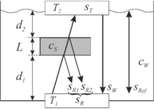
The proposed technique to calculate density is based on the use of simultaneous pulse-echo and through-transmission immersion ultrasonic measurements, which allow the calculation of all required parameters with high accuracy and without any prior knowledge of the material properties [2]. Figure 1 shows the typical immersion set-up in which the transmitterT1is located in the bottom of the water basin, the receiver T2 in the top, and the specimen in between them using a computer controlled XYZ scanner that allows the raster of the material.
Fig. 1. Experiment set-up.
As stated in [2], the advantage of this method is that it only requires three measurements while keeping the layout of the transducers. First, the specimen (variable thickness L and sound velocity cS) is inserted between transducers at appropriate distances (d1andd2). Then, transducer T1sends a pulse and simultaneously reflected and passed through signals are recorded in transducer T1and T2respectively as sR(t) andsT(t). Note thatsR(t) contains reflections from front and back surfaces from the specimen, which will be later gated and separated assR1(t) andsR2(t) respectively. Finally, the specimen is removed and transducer T1 sends a pulse through the water-path, which is received in transducer T2 and recorded as sw(t). Additional water-path measurements are performed changing the distance between transducers for an accurate measurement of the velocity in water.
For any given solid, it is well known that the density S can be calculated as the ratio between the acoustic impedance zS and the sound velocity cS
. S S S z c (1)
The sound velocity can be calculated with an accuracy of millimetres per second using the method developed in [2].
The acoustic impedance of the material can be calculated indirectly using the amplitude of the first echo of the reflected signal. The reflection coefficient RWS between the water and the material can be written as a function of their respective acoustic impedances zS and zW as
. S W WS S W z z R z z (2)
On the other hand, the reflection coefficient can also be written as the ratio between the incident and the reflected signals 1 , R WS Ref A R A (3)
where ARef is the amplitude of the incident wave (note that it is not related to the water-path signal stored assw(t)) and
1
R
A is the peak value of the first reflection in the pulse echo signal,sR1(t).
The density can finally be written as a function of the previous using (3), (2) and (1) as
1 1 , Ref R W S S Ref R A A z c A A (4)
where cS is accurately calculated usingsR(t),sT(t) andsw(t) as described in [2], AR1is the peak of the first echo received in the pulse-echo transducer, and working in a 20º C controlled temperature environment, the acoustic impedance of the distilled water used in the experiments is also known with a constant value of zw1.48MNs m/ . Therefore, the only remaining incognito in (4) is the peak amplitude of the incident wave ARef .
To calculate the incident amplitude we proceed in the same way as we did for the reflected wave, but in this case the material is substituted by air, and signal acquired in transducer T1is now called sRef(t) whose peak amplitude is
Ref
A . Taking into account that the acoustic impedance of air is much smaller than that of water (
1,480,000 / 413.3 /
w Air
z MNs m Ns m z ), the reflection coefficient between them is close to 1 (in magnitude), so all the energy is reflected back to the transducer, therefore the received echo is the incident wave at the water surface distance.
According to the previous, if the material is then placed at exactly the same distance from the transducer as it was from the water surface (d1 in Fig. 1), the ratio between the reflections will provide the desired reflection coefficient between the water and the material that can be used in (4) to calculate the density. It must be taken into account that as both signals have travelled the same distance and have hit the corresponding surface at the same place, the diffraction effects are negligible.
Of course, there are some considerations that have to be taken into account:
1. To avoid the need of corrections, the transducer used in both measurements must be the same, and preferably a focused transducer, using therefore the focal distance as the distance for the water surface and for the material surface.
2. The surfaces of the material and the water must be perpendicular to the transducer. If the surface of the material is not plane, measures could only be taken at particular perpendicular points.
3. Measurements must be taken under controlled temperature environment and with the same fluid (in this case distilled water).
If the above conditions are hold, a 2D map of the densities of the material can be obtained using the scanner, thus providing information about its inner structure and mechanical behaviour locally.
III. EXPERIMENTSET-UP
In order to obtain the desired parameters, an experimental setup was designed according to Fig. 1, in which the transmitter T1 was a 5 MHz wide band focused transducer IRY405 from NDT Transducers LLC and receiver T2 was a composite 5 MHz transducer TF5C6 from Doppler Electronic Technologies. The liquid used was distilled water and temperature was controlled to be at 20º C during all the experiment. The movement of the samples for the 2D scan was made with a 3D scanner designed for that purpose synchronised with the pulser. The resolution in the XY axes was 200 µm per step and 100 µm in the Z axis. The pulser– receiver used was a SE-TX06-00, with a sampling frequency of the acquisition system set to 100 MHz and sampling windows length adjusted in order to have all measurements of each experiment in the same time basis. A 100 ns 5 MHz pulse was used as excitation.
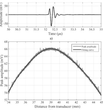
The first step of the method is to calculate a reference signal for the incident wave to be used in (4). For this purpose, and in order to adjust the distance to the actual focal point of the transducer, the tank was slowly filled with water in order to change the distance from the front-face of the transducer to the water surface around the nominal focal distance, which was 38 mm. 4000 signals were obtained between 33 mm and 44 mm controlling the temperature and the stability of the surface.
a)
b)
Fig. 2. (a) – example of reflected signal from water surface and (b) – peak value of the reflected signals as a function of the distance from transducer (black) and its corresponding fitted curve (grey).
Figure 2(a) shows an example of signal acquired from the
surface of the water at a single distance, while Fig. 2(b) shows the peak values of the received echo at each distance (blue line) and the corresponding fitted curve (red line) as a function of the distance of the surface from the transducer T1. As can be seen in Fig. 2(b), the maximum is obtained around 39 mm. The exact calculated focal distance will be the distance at which the flat front surface of the samples will be located for the scanning, therefore this will be the peak value used as ARef .
Then the tank was totally filled and the sample introduced in the liquid. Once the temperature was stabilized, the sample was moved perpendicular to the transducer in steps of 0.5 mm and reflections were used to calculate and average the sound velocity in water according to the procedure described in [2]. Then, the sample is located at the focal distance calculated previously and the scanning starts.
In this experiment 3 different materials were used. The first one was a standard EN-ISO 527-y4 type 1B testing sample of epoxy base provided by a local manufacturer used for the naval industry. The same manufacturer provided also the second sample, a standard EN-ISO 527-y4 type 1B polyester base sample, both with different additives, accelerants and catalysers. The third one was used as reference and was a commercial methacrylate sample 3 cm thick, which according to manufacturer should be flat (in both sides, front and bottom faces) and homogeneous. Figure 3 show pictures of all three samples. Due to their manufacturing process, the polyester and epoxy samples were fabricated using stain steel matrices in which only one face was flat and the other one was left to cure to air, and manually polished after curing, therefore only the front surface of the specimens were flat.
Fig. 3. Specimens used in the analysis.
All 3 specimens were scanned in the same way, acquiring signals in a scanning area of 10 x 10 mm in steps of 0.5 mm, taking 10 measurements at each point and averaging to increase the SNR.
IV. RESULTS
Figure 4 shows the results obtained for the epoxy sample for the sound velocity (Fig. 4(a)), thickness (Fig. 4(b)), acoustic impedance (Fig. 4(c)) and density (Fig. 4(d)) as a function of the scanning point in the X and Y axis in millimetres.
a)
b)
c)
d)
Fig. 4. Epoxy sample: (a) – sound velocity, (b) – thickness, (c) – acoustic impedance and (d) – density.
It can also be seen that the acoustic impedance, and therefore the density, present some abrupt discontinuities,
most of them caused by imperfections in the surface of the samples. These imperfections produce sudden changes in the amplitude of the reflected signal as some of the energy is reflected in different directions, thus the values of the density at these points cannot be trusted and should be rejected.
a)
b)
Fig. 5. Density profiles for (a) – polyester and (b) – methacrylate.
a)
b)
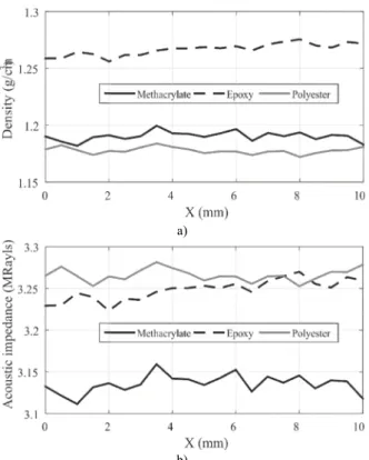
Fig. 6. Comparison between materials for a single scanning line: (a) – density and (b) – acoustic impedance.
This effect is more evident if we observe the density results obtained for the polyester and methacrylate specimens, especially the last one, as shown in Fig. 5(a) and Fig. 5(b) respectively. In this latter case, the discontinuities were caused by scratches produced in the surface with the clamp used to attach the sample in the cutting process.
Apart from these singularities, as expected, the density profile for the industrial methacrylate shows that this material is more homogeneous than the epoxy and polyester samples, that were produced manually mixing the resins and the additives by the manufacturer without a controlled curing process.
Finally, Fig. 6 shows the comparison of the density and the acoustic impedance calculated for each material in a single line free of discontinuities (dotted black line in each density figure indicates the line used for the comparison). Here it can be seen the coincidence between the obtained value of the density for the methacrylate and the mean value provided by the manufacturer (1.19 g/cm3). This figures
show the real potential of this technique for the local and accurate characterization of composites in the manufacturing process.
V. CONCLUSIONS
In this paper we present a new method for calculating the density of solid composites using ultrasound. The method is quite simple and does not require additional calibration or correction of the values obtained. If combined with the proper method for the automatic calculation of the thickness and the sound velocity, it is able to provide automatic and accurate local measurements of the density.
The method is based in the indirect measurement of the incident signal in the material taking advantage of the acoustic properties of water and air, which is at the same time the source of its strength and weakness. The measurement of the reference water reflection is performed only once, because once stored it can be used for any further density measurement of whatever material. Unfortunately, peak amplitude measurements are very sensitive to flatness and temperature, so that the measurements must be performed under controlled conditions.
Concerning the variability with temperature, it may be interesting to repeat the measurements in different temperature conditions to fill a database of water references that can be used as a function of the temperature. The flatness requirement may not have a so easy solution and is a requisite that should be carefully followed. It can also be
extended to the surface of the samples to be analysed. It would also be interesting to calculate the dependence of the parameters with the frequency, as it will provide interesting information about the material mechanical behaviour. According to preliminary analysis, it will be necessary to use spread spectrum signals in order to increase the bandwidth and the energy of the pulses [12].
REFERENCES
[1] L. Svilainis, A. Rodriguez, V. Dumbrava, A. Chaziachmetovas, V. Eidukynas, “Estimation of composite plate attenuation”, Elektronika ir Elektrotechnika, vol. 20, no. 1, pp. 59–62, 2014. [Online]. Available: http://dx.doi.org/10.5755/j01.eee.20.1.4675 [2] A. Rodriguez, L. Svilainis, V. Dumbrava, A. Chaziachmetovas,
A. Salazar, “Automatic simultaneous measurement of phase velocity and thickness in composite plates using iterative deconvolution”, NDT&E International, vol. 66, pp. 117–127, 2014. [Online]. Available: http://dx.doi.org/10.1016/j.ndteint.2014.06.001
[3] H. Wang et al., “The design of the ultrasonic liquid density measuring instrument”, in Third Int. Conf. Measuring Technology and Mechatronics Automation, vol. 3, 2011, pp. 758–760. [Online]. Available: http://dx.doi.org/10.1109/ICMTMA.2011.762
[4] R. C. Asher, “Ultrasonics in chemical analysis”,Ultrasonics, vol. 25, pp. 17–19, 1987. [Online]. Available: http://dx.doi.org/10.1016/0041 -624X(87)90004-7
[5] J. M. Hale, “Ultrasonic density measurement for process control”, Ultrasonics, vol. 26, no. 6, pp. 356–357, 1988. [Online]. Available: http://dx.doi.org/10.1016/0041-624X(88)90036-4
[6] A. Puttmer, P. Hauptmann, B. Henning, “Ultrasonic density sensor for liquids”, IEEE Trans. Ultrason., Ferroelectr. Freq. Contr., vol. 47, no. 1, pp. 85–92, 2000. [Online]. Available: http://dx.doi.org/10.1109/58.818751
[7] R. T. Higuti, J. C. Adamowski, “Ultrasonic densitometer using a multiple reflection technique”, IEEE Trans. Ultrason., Ferroelectr. Freq. Contr. vol. 49, no. 9, pp. 1260–1268, 2002. [Online]. Available: http://dx.doi.org/10.1109/TUFFC.2002.1041543
[8] D. J. McClements, P. Fairly, “Ultrasonic pulse echo reflectometer”, Ultrasonics, vol. 29, pp. 58–62, 1991. [Online]. Available: http://dx.doi.org/10.1016/0041-624X(91)90174-7
[9] M. S. Greenwood, “Ultrasonic fluid densitometer having liquid/wedge and gas/wedge interfaces”, U.S. Patent 6.082.181, July 2000.
[10] S. Hoche, M. A. Hussein, T. Becker, “Ultrasound-based density determination via buffer rod techniques: a review”,J. Sens. Sens. Syst. vol. 2, pp. 103–125, 2013. [Online]. Available: http://dx.doi.org/10.5194/jsss-2-103-2013
[11] S. Hoche, M. A. Hussein, T. Becker, “Density, ultrasound velocity, acoustic impedance, reflection and absorption coefficient determination of liquids via multiple reflection method”,Ultrasonics, vol. 57, pp. 65–71, 2015. [Online]. Available: http://dx.doi.org/ 10.1016/j.ultras.2014.10.017
[12] L. Svilainis, S. Kitov, A. Rodriguez, L. Vergara, V. Dumbrava, A. Chaziachmetovas, “Comparison of spread spectrum and pulse signal excitation for split spectrum techniques composite imaging”, in IOP Conf. Series: Materials Science and Engineering, vol. 42, no. 1, 2012. [Online]. Available: http://dx.doi.org/10.1088/1757-99X/42/1/012007