Uniform Sampling Framework for Sampling Based Motion Planning and Its Applications to Robotics and Protein Ligand Binding

(1)

UNIFORM SAMPLING FRAMEWORK FOR SAMPLING BASED MOTION PLANNING AND ITS APPLICATIONS TO ROBOTICS AND PROTEIN

LIGAND BINDING

A Dissertation by HSIN YI YEH

Submitted to the Office of Graduate and Professional Studies of Texas A&M University

in partial fulfillment of the requirements for the degree of DOCTOR OF PHILOSOPHY

Chair of Committee, Nancy M. Amato Committee Members, J. Martin Scholtz

Dezhen Song Tiffani L. Williams Head of Department, Dilma Da Silva

May 2016

Major Subject: Computer Science

(2)

ABSTRACT

Sampling-based motion planning aims to find a valid path from a start to a goal by sampling in the planning space. Planning on surfaces is an important problem in many research problems, including traditional robotics and computational biology. It is also a difficult research question to plan on surfaces as the surface is only a small subspace of the entire planning space. For example, robots are currently widely used for product assembly. Contact between the robot manipulator and the product are required to assemble each piece precisely. The configurations in which the robot fingers are in contact with the object form a surface in the planning space. However, these configurations are only a small proportion of all possible robot configurations. Several sampling-based motion planners aim to bias sampling to specific surfaces, such asCobst surfaces, as needed for tasks requiring contact, or along the medial axis,

which maximizes clearance. While some of these methods work well in practice, none of them are able to provide any information regarding the distribution of the samples they generate. It would be interesting and useful to know, for example, that a particular surface has been sampled uniformly so that one could argue regarding the probability of finding a path on that surface. Unfortunately, despite great interest for nearly two decades, it has remained an open problem to develop a method for sampling on such surfaces that can provide any information regarding the distribution of the resulting samples.

Our research focuses on solving this open problem and introduces a framework that is guaranteed to uniformly sample any surface in Cspace. Instead of explicitly

(3)

sam-pling framework only requires detecting intersections between a line segment and the target surface, which can often be done efficiently. Intuitively, since we uni-formly distribute the line segments, the intersections between the segments and the surfaces will also be uniformly distributed. We present two particular instances of the framework: Uniform Obstacle-based PRM (UOBPRM) that uniformly samples Cobst

surfaces, and Uniform Medial-Axis PRM (UMAPRM) that uniformly samples the Cspace medial axis. We provide a theoretical analysis for this framework that

estab-lishes uniformity and probabilistic completeness and also the probability of sampling in narrow passages. We show applications of this uniform sampling framework in robotics (both UOBPRM and UMAPRM) and in biology (UOBPRM). We are able to solve some difficult motion planning problems more efficiently than other sam-pling methods, including PRM, OBPRM, Gaussian PRM, Bridge Test PRM, and MAPRM. Moreover, we show that UOBPRM and UMAPRM have similar computa-tional overhead as other approaches. UOBPRM is used to study the ligand binding affinity ranking problem in computational biology. Our experimental results show that UOBPRM is a potential technique to rank ligand binding affinity which can be further applied as a cost-saving tool for pharmaceutical companies to narrow the search for drug candidates.

(4)

DEDICATION

To my parents: you are always my strong foundation

(5)

ACKNOWLEDGEMENTS

I would first like to thank my advisor, Dr. Nancy Amato, for her support and encouragement. I deeply appreciate all her guidance and care through the years.

I would also like to thank my committee members, Dr. J. Martin Scholtz, Dr. Dezhen Song, and Dr. Tiffani L. Williams, for their support and feedback. I appre-ciate they committed their time to help me grow as a researcher.

I also thank all the collaborators that I have worked with over the years, both on this work and on other research projects: Jory Denny, Chinwe Ekenna, Mukulika Ghosh, Aaron Lindsey, Dr. Lydia Tapia, Dr. Shawna Thomas, and Chih-Peng Wu. I am especially thankful to Shawna for her guidance over the years. Thank you for your extreme patience as I explored research problems in motion planning and computational biology. I am also grateful for working with Chinwe and Mukulika through most of my graduate career. Since we’ve shared an office together, we col-laborated not only on research but also the service in AWICS. We have accomplished a lot by working together.

Thank you to all the Parasol members, both former and current.

Thanks to Texas A&M University Diversity Fellowship who have supported my graduate career. I would also like to thank all the conferences and workshops that provided travel grants during my graduate career. These include funding to attend the Grace Hopper Celebration of Women in Computing Conference, the IEEE/RSJ International Conference on Intelligent Robots and Systems, the IEEE International Conference on Robotics and Automation, and the ACM Conference on Bioinfor-matics, Computational Biology, and Health Informatics. It helped to broaden my view.

(6)

Finally, I would like to thank my family who always support me and stay with me through my graduate career. My parents taught me the value of the hard work. Their encouragement helped me throughout this long journey. My brother, Shu-Hao, has been the one who always reminds me the joy of learning new things. Thank you for always providing me the courage of facing new challenges.

(7)

3. UNIFORM SAMPLING FRAMEWORK . . . 16

3.1 Uniformly Generate Configurations in Cspace . . . 16

3.1.1 Bounding Box Adjustment . . . 17

3.2 Uniformity . . . 18

3.3 Probabilistic Completeness . . . 18

3.4 Uniform Sampling in Passages . . . 21

4. UNIFORM OBSTACLE-BASED PRM (UOBPRM) . . . 23

4.1 Detecting Surface Membership . . . 23

(8)

4.2 UOBPRM v.s. Gaussian PRM . . . 26

4.3 Experiment Results . . . 29

4.3.1 Planners Studied . . . 30

4.3.2 Uniformity . . . 30

4.3.3 Cost . . . 40

4.3.4 Narrow Passage Analysis . . . 43

4.3.5 Motion Planning . . . 46

4.3.6 UOBPRM and Gaussian Sampling Performance Comparison . 47 5. UNIFORM MEDIAL-AXIS PRM (UMAPRM) . . . 53

5.1 Detecting Surface Membership . . . 53

5.1.1 Bounding Box Adjustment . . . 54

5.2.1 Planners Studied . . . 57

5.2.2 Implementation Detail for Point Robot . . . 57

5.2.3 Uniformity . . . 58

5.2.4 Cost . . . 61

5.2.5 Narrow Passage Analysis . . . 62

5.2.6 Motion Planning . . . 65

6. RANK LIGAND BINDING AFFINITY . . . 68

6.1 Preliminaries . . . 69

6.1.1 Ligand Binding Affinity . . . 69

6.1.2 Modeling Molecular Motions . . . 73

6.2 Method . . . 74

6.2.1 Protein and Ligand Models . . . 75

6.2.2 Using UOBPRM to Rank Binding Affinity . . . 75

6.2.3 Affinity Metrics . . . 78

6.3.1 Target Protein 3W6H . . . 79

6.3.2 Target Protein 4RRW . . . 80

6.3.3 Target Protein 4K5Y . . . 81

7. CONCLUSION AND FUTURE WORK . . . 87

(9)

LIST OF FIGURES

FIGURE Page

1.1 (a) A KUKA youBot [43] needs to pass through the narrow passage caused by the surrounding obstacles in order to approach to the en-trance to the next room. (b) Planning on the medial axis in the narrow passage provides a high clearance path since the medial axis is a surface that is equidistant to two or more obstacles. . . 2 1.2 (a) Binding between the protein 1UYX and two ligands. (b) The

binding pocket (binding site) is a small region on the protein surface where the ligand can form chemical bonds to cause some biochemical effects. The images were generated with PyMOL [25]. . . 3 1.3 Nodes generated by (a) PRM [40], (b) UOBPRM [22], (c) UMAPRM [73],

(d) OBPRM [2], (e) Gaussian PRM [13], (f) Bridge Test PRM [32], and (g) MAPRM [68] in a simple 2D environment containing two parallel obstacles. PRM, UOBPRM, and UMAPRM can guarantee uniformly distributed samples on their respective targeted surfaces. . 4 2.1 The configuration distribution of OBPRM (in blue) is biased by (a)

the shape of the Cobst and (b) the position of the initial colliding

con-figuration cin (in red). . . 10

3.1 Ris the target surface where uniform samples are distributed. The red dashed line represents the small portion Rp,ǫ onR where the line

seg-ment (c, l−→d) crossesR. pis the intersection between the line segment and R. Therefore, the probability of a line segment intersecting the target surface is the probability that one endpoint of the line segment resides in a sphere with radius l centered atpand the−→d intersects Rp,ǫ. 19

4.1 Finding intersections between the line segment and the obstacle by checking the validity of intermediate configurations along segment. The valid one is retained at every validity change. Here, the valid nodes that are retained are solid [22]. . . 24

(10)

4.2 The target surface R is the Cf ree around Cobst. p is the intersection

between the line segment (c, l−→d) and the target surface which will be retained as a roadmap node. Since the line segments are uniformly distributed in the Cspace, the intersections found in R along the line

segments are also uniformly distributed [22]. . . 25 4.3 In this example, the uniformity guarantee is broken for

UOBPRMbe-cause the original bounding box (solid line) is too close to the Cobst

in the upper left and bottom right corners. This restricts the line segments that can be placed in the red regions. The bounding box is extended to the dashed line to allow all segments of length l that could intersect the Cobst. . . 26

4.4 The example environment where directly expanding the bounding box by the line segment length l wastes time in generating line segments that can not find intersections in the targeted region. The solid line shows the original bounding box, the dashed line shows the bound-ing box directly expanded by l and the dotted line is the adjusted bounding box we perform. . . 28 4.5 Four environments are used to compare the distribution of samples

produced by UOBPRM and other sampling methods. The robot is a small cube. . . 31 4.6 Sample distribution example in the single ball environment. UOBPRM

has the most uniformly distributed samples around the obstacle surfaces. 33 4.7 Distribution comparison of ball (red) and free (blue) regions in the

single ball environment. Ideal percentage for ball is 25% and free is 0%. 34 4.8 Sample distribution example in the 4 balls environment. . . 35 4.9 Distribution comparison in the environment with 4 balls of equal size,

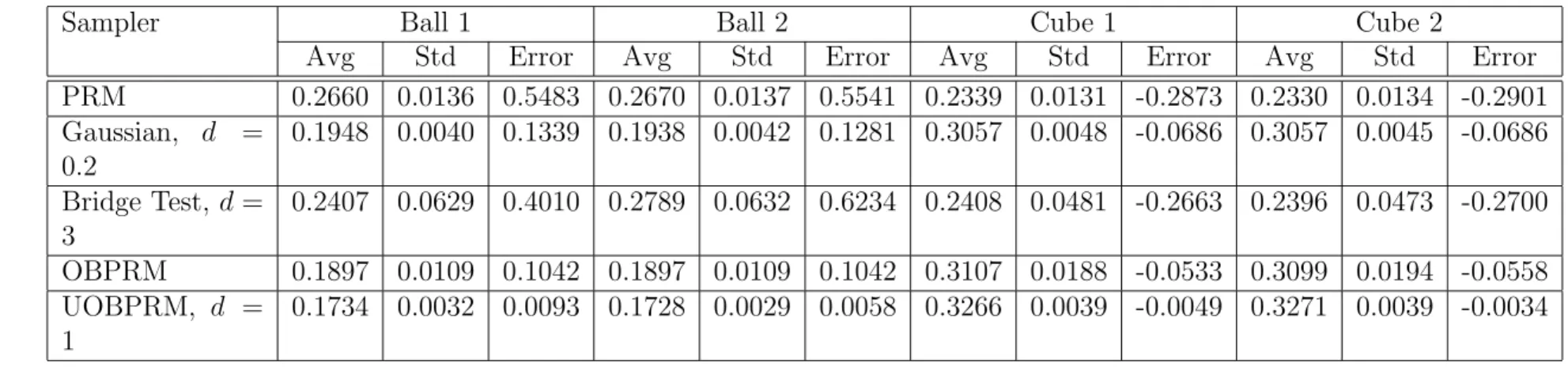
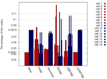
each ball is a different color. Ideal percentage is 6.25%. UOBPRM and Gaussian sampling generate more uniformly distributed samples than the others. . . 35 4.10 Sample distribution example in the mixture environment. . . 37 4.11 Distribution comparison of ball (red) and cube (blue) regions in the

en-vironment with a mixture of balls and cubes. Ideal percentage for ball is 4.31% and cube is 8.19%. The sample distribution for UOBPRM is the most uniform. . . 39

(11)

4.12 Normalized distribution error between different samplers. UOBPRM has the lowest distribution error among other samplers. . . 40 4.13 Environments that vary the narrow passage width. Passage 1 is the

easiest problem and Passage 3 is the most difficult problem. The robot is a small cube. . . 43 4.14 (a) Number of samples inside the narrow passage. (b) Time it takes

to generate 1000 samples in the roadmap. ⋆ stands for infinity value as Bridge Test PRM is not able to generate any sample in the en-vironment given the line segment length too short to bridge the gap between obstacles. (c) Percentage of samples in the narrow passage. The surface area ratio between the narrow passage and the Cobst is

0.4444. Only UOBPRM’s performance is comparable. . . 49 4.15 (a) Number of samples in the map in order to generate 100 samples

inside the narrow passage. (b) Time it takes to generate the configu-rations. ⋆ indicates the infinity time that Bridge Test PRM needs in Passage 1 since the line segment length is not long enough to bridge the obstacles. . . 50 4.16 Two environments are used for the study of the motion planning

prob-lems. The robot is a small cube. . . 50 4.17 A relatively free environment is used to study the relationship between

UOBPRM and Gaussian sampling. The robot is a small cube. . . 50 4.18 Time required to generate 4000 nodes by UOBPRM and Gaussian

sampling with different line segment lengths (l in UOBPRM and din Gaussian sampling). Step size t is equal to line segment length. Both methods perform similarly when the line segment length is short, and UOBPRM is more efficient than Gaussian sampling when the line segment length is long. . . 51 4.19 Distribution comparison of ball (red) and free (blue) regions. Ideal

percentage of ball is 25% and free is 0%. . . 52 5.1 The configurations and their closest obstacles. The medial axis is

given by the dashed line. Different colors represent different closest obstacles. The closest obstacle is changed when the medial axis is crossed. . . 54 5.2 An example showing that more than one crossing point can be

(12)

5.3 The target surface R is the Cf ree along the medial axis (dashed line).

p is the intersection between the line segment (c, l−→d) and the target surface which will be retained as a roadmap node. Since line segments are uniformly distributed in the Cspace, the intersections found in R

along the line segments are also uniformly distributed [73]. . . 55 5.4 An example illustrating the situation when the uniformity guarantee

is broken. The original bounding box (solid line) is too close to the medial axis, restricting the line segments that can be placed in the Cspace. The bounding box is extended to the dashed line to allow all

segments of length l that could intersect the medial axis. . . 56 5.5 Three examples showing how UMAPRM finds configurations on the

medial axis for a point robot by checking changes in closest triangles on obstacles. The grey face is the medial axis. The medial axis is crossed when (a) closest triangles are on different obstacles, (b) closest triangles are on the same obstacle but not adjacent to each other, or (c) neighboring concave triangles are on the same obstacle [73]. . . 58 5.6 (a, b) Two environments used to compare the distribution of UMAPRM

and MAPRM. (c, d, e) Narrow passages of varying surrounding obsta-cle volume to compare sampling densities of UMAPRM and MAPRM. The robot we study in every environment is a point robot. . . 59 5.7 The average of standard deviations of distances between each node and

its closest neighbor for roadmaps of 1000 samples between UMAPRM (green), MAPRM (blue), and uniform random sampling on the medial axis (red) [73]. . . 60 5.8 Distribution of 1000 samples generated by UMAPRM, MAPRM, and

uniform random sampling in the 2D Block environment [73]. . . 61 5.9 Distribution of 1000 samples generated by UMAPRM, MAPRM, and

uniform random sampling in the 3D Block environment [73]. . . 61 5.10 The time to generate 1000 samples for UMAPRM and MAPRM in

Obstacle 1, 2, and 3 [73]. . . 62 5.11 (a) Number of samples inside the narrow passage. (b) Time it takes

to generate 1000 samples in the roadmap. . . 63 5.12 (a) Number of samples in the map in order to generate 100 samples

inside the narrow passage. (b) Time it takes to generate the configu-rations. . . 64

(13)

5.13 Motion planning environments studied. The robot is a point robot for all environments. (a) 2DMaze. The start and the goal reside at the two ends in the free space. (b) STunnel. The start and the goal are in the top left and the bottom right corners. (c) 2DHeterogeneous. The start is in the top free space and the goal is placed in the bottom cluttered region. (d) Bug Trap. The objective is to get out of the trap through the narrow passage. . . 66 5.14 The time to solve the problem for UMAPRM, MAPRM, and PRM in

different environments [73]. . . 66 5.15 The average clearance of the path for UMAPRM, MAPRM, and PRM

in different environments [73]. . . 67 6.1 A protein (shown in wireframe) with a ligand (shown in spheres)

bound inside it. . . 69 6.2 The lock-and-key ligand binding model: (a) A ligand successfully

binds to the target protein due to complementary geometry and chem-istry. (b) The ligand is incompatible and the protein-ligand complex cannot form. . . 70 6.3 In the induced-fit model, the protein undergoes a conformational change

when ligand binds to it. The shape of the ligand becomes complemen-tary to the shape of the binding site after the ligand binds to the protein. . . 71 6.4 Protein 3W6H in wireframe (a) and in spheres (b) viewed by

Py-MOL [25]. (c) The protein is modeled as a rigid obstacle. (d)-(h) Varying numbers of ligand samples (ligand centers of mass only shown). 76 6.5 Protein 4RRW in wireframe (a) and in spheres (b) viewed by

Py-MOL [25]. (c) The protein is modeled as a rigid obstacle. (d)-(h) Varying numbers of ligand samples (ligand centers of mass only shown). 83 6.6 Protein 4K5Y in wireframe (a) and in spheres (b) viewed by

Py-MOL [25]. (c) The protein is modeled as a rigid obstacle. (d)-(h) Varying numbers of ligand samples (ligand centers of mass only shown). 84 6.7 Ligand candidates from PubChem [12] for protein 3W6H (see

Fig-ure 6.4(a)) ordered by binding affinity rank best to worst. . . 84 6.8 Ligand candidates from PubChem [12] for protein 4RRW (see

(14)

6.9 Ligand candidates from PubChem [12] for protein 4K5Y (see Fig-ure 6.6(a)) ordered by binding affinity rank best to worst. . . 86

(15)

LIST OF TABLES

TABLE Page

4.1 Average and standard deviation of ball and free space in single ball environment for different samplers. The ideal average for ball is 0.25 and free is 0. Error is calculated as the % difference to ideal. . . 33 4.2 Average and standard deviation of each ball obstacle in the

environ-ment with 4 balls of equal size for different samplers. The ideal average for ball is 0.25. Error is calculated as the % difference to ideal. . . 36 4.3 Average and standard deviation of ball and cube obstacle in the

envi-ronment with a mixture of balls and cubes for different samplers. The ideal average for ball is 0.1718 and cube is 0.3282. Error is calculated as the % difference to ideal. . . 38 4.4 Generation time for various samplers and input parameters in the

single ball environment [22]. . . 41 4.5 Generation time for various sampling methods and input parameters

in the Tunnel environment [22]. . . 42 4.6 Time required to solve the heterogeneous Tunnel environment query

by different robots for various sampling methods and input parame-ters. There are two types of robots: R for rigid body and L for linkage robot. . . 47 4.7 Time required to solve the Z-Tunnel environment query by different

sampling methods. . . 48 6.1 Comparison of published binding affinity ranking and approximated

binding affinity ranking for 3W6H. . . 80 6.2 Comparison of published binding affinity ranking and approximated

binding affinity ranking for 4RRW. . . 81 6.3 Comparison of published binding affinity ranking and approximated

(16)

1. INTRODUCTION

The motion planning problem is to find a valid (e.g., collision free) trajectory for a movable object (robot) from a start position to a goal position. Motion planning has been studied extensively and has various applications such as robotics [11, 34, 42], computer animation [41, 6], computer-aided design (CAD) [18, 59], and computa-tional biology [57, 4, 1, 63]. Motion planning is very difficult, known to be intractable for even very simple problems [55, 5]. Consequently, randomized sampling-based planners have become the state-of-the-art methods for planning [40, 34, 47, 46, 2, 3, 13, 32, 68, 49, 30, 72, 50]. These planners build graphs [40] or trees [34, 47] that approximate the topology of the planning space and encode representative feasible trajectories.

The focus of this dissertation is to study motion planning on surfaces. This is a challenging and important problem with applications in many research areas, including traditional robotics and computational biology. The dimension of a surface is one less than the dimension of the planning space, hence sampling on the surface can be difficult because the surface is a relatively small space compared to the entire planning space. For example, robots are widely used for product assembly nowadays. In order to precisely assemble each piece, contact between the robot manipulator and the product are required. The configurations in which the robot fingers are in contact with the object form a surface in the planning space. However, these configurations are only a small percentage of all possible robot configurations. Therefore, it is very difficult to obtain such configurations with sampling-based planners.

Many problems in robotics require robots to operate in cluttered environments with narrow passages. For example, as shown in Figure 1.1(a), a KUKA youBot [43]

(17)

tries to get to the next room by passing through a narrow passage. As the robot is very close to the surrounding obstacles, even small movements can cause the robot to collide with obstacles. The medial axis is a surface that maximizes clearance and hence, planning paths on medial axis surfaces is desirable for many applications (Figure 1.1(b)). Another example is when the task requires contact between the robot and an object; since the robot configurations that are in contact with the object form a surface in the planning space, this is a planning problem in which paths must be found on this surface.

(a) (b)

Figure 1.1: (a) A KUKA youBot [43] needs to pass through the narrow passage caused by the surrounding obstacles in order to approach to the entrance to the next room. (b) Planning on the medial axis in the narrow passage provides a high clearance path since the medial axis is a surface that is equidistant to two or more obstacles.

Planning on surfaces also has applications in computational biology. One example is the ligand binding problem. Protein-ligand interaction is essential to understand many biological mechanisms. The efficiency of a drug (ligand) molecule is determined by its ability to find a specific position and orientation on the protein surface, more specifically, on the surface in the binding pocket (binding site, see Figure 1.2(b)). This contact (called binding) on the protein surface can either activate or inhibit

(18)

some biochemical effects. For example, the binding between insulin and the insulin receptor will trigger some intracellular insulin effects, such as fat metabolism and glucose uptake [56]. Planning the ligand motion as it approaches and then attaches to the protein surface is a motion planning problem requiring contact. Sampling-based motion planning can also be used in ligand binding site prediction, which helps to predict where on the protein surface the ligand may form contact and trigger biochemical effects [71, 70, 67, 15, 16]. Sampling-based motion planning can be used to map the planning space of the protein, which can be utilized to predict binding sites (Figure 1.2(a)).

(a) (b)

Figure 1.2: (a) Binding between the protein 1UYX and two ligands. (b) The binding pocket (binding site) is a small region on the protein surface where the ligand can form chemical bonds to cause some biochemical effects. The images were generated with PyMOL [25].

Many motion planning methods have been specialized for planning on or near surfaces, such as near obstacle surfaces [2, 13, 32] or along medial axis surfaces [68, 49], to improve performance or to find paths with desirable properties (e.g., high clearance). OBPRM [2] (Figure 1.3(d)) was the first method targeting sampling on obstacle surfaces, and then Gaussian PRM [13] (Figure 1.3(e)) and Bridge Test

(19)

PRM [32] (Figure 1.3(f)) were proposed to generate samples on obstacle surfaces or in narrow passages, respectively. MAPRM [68] (Figure 1.3(g)) biases sampling towards medial axis surfaces. While some of these methods work well in practice, none of them is able to provide any information regarding the distribution of the samples it generates. It would be interesting and useful to know, for example, that a particular surface has been sampled uniformly so that one could argue regarding the probability of finding a path on that surface. Unfortunately, despite great interest for nearly two decades, it has remained an open problem to develop a method for sampling on such surfaces that can provide any information regarding the distribution of the resulting samples.

(a) (b) (c)

(d) (e) (f) (g)

Figure 1.3: Nodes generated by (a) PRM [40], (b) UOBPRM [22], (c) UMAPRM [73], (d) OBPRM [2], (e) Gaussian PRM [13], (f) Bridge Test PRM [32], and (g) MAPRM [68] in a simple 2D environment containing two parallel obstacles. PRM, UOBPRM, and UMAPRM can guarantee uniformly distributed samples on their respective targeted surfaces.

(20)

1.1 Research Contribution

In this dissertation, we present a solution to a long standing open problem and develop a general method that can uniformly sample surfaces. Instead of explicitly constructing the target surfaces, which is generally intractable, our uniform sampling framework only requires detecting intersections between a line segment and the target surface, which can often be done efficiently. Intuitively, since we uniformly distribute the line segments, the intersections between the segments and the surfaces will also be uniformly distributed.

We use the uniform sampling framework in sampling-based motion planning to study some important surfaces in the planning space. Uniform Obstacle-based PRM (UOBPRM) [22] is the first example of our framework which samples obstacle sur-faces uniformly (Figure 1.3(b)). Uniform Medial-Axis PRM (UMAPRM) [73] is another example whose target surfaces are the medial axis of Cspace (Figure 1.3(c)).

We show that this framework generates configurations uniformly distributed on the target surfaces of Cspace (all possible robot placements), both experimentally and

theoretically. We prove that the probability of sampling the target surfaces is pro-portional to their surface area, which leads to important observations regarding the probability of generating samples in narrow passages. Next, we prove that the uni-form sampling framework is probabilistically complete. We also uni-formalize the rela-tionship between UOBPRM and Gaussian PRM [13] and show that Gaussian PRM is a special case of UOBPRM with particular parameter settings.

We show applications of this uniform sampling framework in robotics (both UOBPRM and UMAPRM) and in biology (UOBPRM). We are able to solve some difficult motion planning problems more efficiently than other sampling methods, including PRM [40], OBPRM [2], Gaussian PRM [13], Bridge Test PRM [32], and

(21)

MAPRM [68]. Our results show that both UOBPRM and UMAPRM have negli-gible computational overhead over other sampling techniques and UMAPRM can solve problems that others could not (e.g., a bug trap environment). We illustrate how UOBPRM can be used to study the ligand binding affinity ranking problem by generating uniformly distributed ligand samples on the target protein’s surfaces. Experiments with several target proteins using two different experimental measures for binding affinity show that UOBPRM can potentially rank binding affinities for different ligands.

In summary, our contributions include a uniform sampling framework that uni-formly generates configurations on surfaces and its instances for different target sur-faces (e.g., Cobst surfaces and medial axis surfaces). We evaluate the framework on a

variety of applications. More specifically, our contributions are as follows:

• We present a general uniform sampling framework that distributes samples uniformly on surfaces and provide examples of this framework forCobst surfaces

(UOBPRM) and medial axis surfaces (UMAPRM).

• We provide theoretical guarantees on the distribution of samples obtained by our method and prove that it preserves probabilistic completeness of sampling-based motion planners and performs stably with respect to changes in the narrow passage volume (UOBPRM) or in the surrounding obstacle volume (UMAPRM).

• We show applications of the uniform sampling framework in robotics (both UOBPRM and UMAPRM) and in biology (UOBPRM).

Portions of this research were previously published and presented. UOBPRM, which generates uniformly distributed configurations around Cobst surfaces, was

(22)

Robots and Systems (IROS) [22]. UMAPRM, which uniformly samples the medial axis, was published in the proceedings of the 2014 IEEE International Conference on Robotics and Automation (ICRA) [73].

1.2 Outline

This dissertation is organized as follows. In Chapter 2, we provide background on sampling-based motion planning. We discuss several sampling methods that bias the sampling to specific surfaces (e.g., near Cobst boundaries or medial axis).

In Chapter 3, we present a uniform sampling framework that provably distributes samples uniformly on surfaces in Cspace. We provide theoretical guarantees that it

preserves probabilistic completeness of sampling-based motion planners and has a higher probability of sampling narrow passages. Chapter 4 presents UOBPRM as one specific instance from the uniform sampling framework that distributes samples uniformly aroundCobstsurfaces. We demonstrate that UOBPRM generates uniformly

distributed samples and improves the efficiency to solve the motion planning prob-lems. The relationship between UOBPRM and Gaussian PRM is compared both theoretically and experimentally. Chapter 5 presents another instance of the uni-form sampling framework, UMAPRM, that generates the samples uniuni-formly along the medial axis in Cf ree. We evaluate the uniformity and the efficiency of UMAPRM

against MAPRM. In Chapter 6, we show how we apply the uniform sampling frame-work to study the ligand binding affinity ranking problem. We present the results on three different target proteins and compare against experimentally determined ranking. We conclude with some final remarks in Chapter 7.

(23)

2. PRELIMINARIES AND RELATED WORK

In this chapter, we discuss motion planning preliminaries and existing sampling-based approaches. We limit the discussion to methods focused on planning on par-ticular surfaces, such as narrow passages and along the medial axis of the freeCspace.

2.1 Motion Planning

A robot is a movable object that can be described by n parameters (degrees of freedom, dofs) and each parameter represents an object component, such as position and orientation. All possible robot placements (or configurations) form an n-dimensional space, called configuration space (Cspace). Each robot configuration is

represented as a point hx1, x2, ..., xni where xi is the ith dof in Cspace. All feasible

robot configurations formCf ree, andCobst is the union of all infeasible configurations.

The motion planning problem is to find a path in Cf ree from a start configuration

to a goal configuration. It is usually not feasible to compute the Cobst boundaries

explicitly. However, we can utilize simple collision detection in the workspace (e.g., the actual space where the robot moves) to determine whether the configuration is valid or not.

Exact solutions are computationally infeasible, especially when the robot has many dofs [5]. Some randomized algorithms have been developed to address this issue, e.g., sampling-based methods [40, 46] which solve many previously intractable problems. Specifically, Probabilistic RoadMap methods (PRMs) [40] construct a graph, or roadmap, to represent Cf ree by randomly sampling configurations and

re-taining valid ones. A simple local planner is applied to connect the configuration to its closest neighbors to form a roadmap. During the query process, the start and the goal configurations are added to the roadmap, connected by a local planner, and a

(24)

graph search algorithm, e.g, Dijkstra’s algorithm, extracts the solution path. PRMs have been shown to mapCf ree efficiently but are not good at mapping some particular

regions in Cspace, such as in narrow passages and along the medial axis [33].

2.2 Obstacle-Based Sampling

The probability of generating a sample in a particular region of Cspace for the

traditional uniform sampling [40] depends on the ratio of the region volume to the Cspace volume. A narrow passage is a region in Cspace of a volume so small that

uniform random sampling is unlikely to generate any configuration in it [35] but that is important for planning, e.g., when solution paths are required to pass through it. Since Cobst surfaces define the boundaries of narrow passages, many PRM variants

have been proposed to sample on those surfaces to increase coverage in these difficult regions. Here we discuss three approaches designed to address this issue: OBPRM, Gaussian PRM, and Bridge Test PRM.

2.2.1 OBPRM

Obstacle-Based PRM (OBPRM) [2] tries to generate samples close to obstacle surfaces. Algorithm 1 describes how OBPRM generates samples. It first finds a configuration cin colliding with the obstacles. A random ray originated at cin is

selected and a free node c1 is found along that ray. The boundary point is found by a bisection search between cin and c1. The boundary configurations will be kept as

the roadmap nodes. Figure 1.3(d) shows samples generated by OBPRM.

Although OBPRM can generate configurations close to Cobst surfaces, the node

distribution is dependent on the Cobst shape and the position of the initial invalid

configuration cin, as shown in Figure 2.1. There is no perfect position for the initial

colliding configuration to guarantee uniform node distribution if the shape of theCobst

(25)

Algorithm 1 OBPRM: Obstacle-Based PRM Sampler(n) Input: A maximum number of attempts n and a step size t Output: A set of nodes V near obstacles surfaces

1: V =∅

2: for i= 0 →n do

3: Randomly generate a point cin in a Cobst

4: Randomly select a point c1 in Cspace

5: Letci =cin

6: while ci not in Cf ree & ci in Cspace do

7: Increment ci by step sizet along direction−−→cinc1

8: if ci inCspace then

9: Bisect between ci and ci−1 to find free boundary point cout

10: Add cout toV

11: return V

be uniformly distributed on the obstacle surfaces if the initial colliding configuration does not reside at the center of the Cobst (see Figure 2.1(b)). In particular, the

portion of the surface closer to the initial colliding configuration will have a denser node distribution.

(a) (b)

Figure 2.1: The configuration distribution of OBPRM (in blue) is biased by (a) the shape of the Cobst and (b) the position of the initial colliding configuration cin (in

red).

Some work has been proposed to use workspace information to achieve a better node distribution [3]. The heuristics help to bias the initial colliding configuration

(26)

selection. The point representing an object (a robot or an obstacle) can be selected in different ways that will affect how the samples are biased. For example, using a random vertex to represent an object will bias node generation towards the portions of the object with more vertices. Selecting a triangle with probability proportional to its area and representing the object by a random vertex in that triangle can bias the sampling towards triangles with larger area. After selecting the points associated with the objects based on these heuristics, the robot is translated in order to coincide with the selection points of the robot and the obstacle and is rotated until finding the initial colliding configuration. Although the results show that these proposed heuristics can improve the node distribution, there are still no guarantees about the configuration distribution around Cobst surfaces.

2.2.2 Gaussian PRM

Gaussian PRM [13] attempts to generate configurations that are a Gaussian dis-tanced away from the obstacle surfaces. A first configuration is randomly generated and the second is generated a Gaussian distance d away from the first configuration, where d is a user-specified parameter. If the validities of the two configurations are different, then the valid one will be retained as a node in the roadmap. Otherwise, both are discarded. Algorithm 2 illustrates the process and Figure 1.3(e) shows an example of Gaussian samples.

Gaussian PRM can be much slower and generate fewer samples than PRM in the same number of attempts since Gaussian PRM will discard many configurations that PRM would retain. Also, Gaussian PRM can be costly since it may be difficult to generate nodes with different validities. Roadmap quality is highly dependent on howd is selected. Ifdis too small, it is very likely that the configuration is too close to the Cobst causing collision. When d is large, the configurations are too far from

(27)

Algorithm 2 Gaussian PRM Sampler(n, d)

Input: A maximum number of attempts n and a distance d

Output: A set of nodes V a Gaussian distanced away from obstacle surfaces 1: V =∅

2: for i= 1 →n do

3: Randomly select a configurationc1

4: Generate configurationc2 a Gaussian distance d along a random ray from c1 5: if the validity of c1 and c2 are different then

6: Add the valid one to V 7: return V

the Cobst surfaces. Gaussian PRM has an unknown node distribution.

2.2.3 Bridge Test PRM

Bridge Test PRM [32] has a similar node generation process to Gaussian PRM [13]. It also utilizes validity checking to bias sampling to the difficult regions, such as near Cobst surfaces and narrow passages. Algorithm 3 provides the pseudocode for Bridge

Test PRM. It first generates an invalid configuration, and a second configuration is sampled a distance d away. If the second configuration is also invalid, the midpoint is found and its validity checked. The midpoint will be retained as a roadmap node if it is valid. Figure 1.3(f) shows an example roadmap generated by Bridge Test PRM. Bridge Test PRM takes longer than OBPRM and Gaussian PRM since it needs to generate three consecutive samples in which the midpoint is valid and the endpoints are invalid. Bridge Test PRM also suffers from tuning the parameter d which can greatly affect the performance and the quality of the sampler. Finally, it has an unknown node distribution around Cobst surfaces.

2.3 Medial Axis Sampling

Most methods aim to simply find a feasible path. This may lead to paths with low clearance that may be a high risk for some applications. For example, OBPRM,

(28)

Algorithm 3 Bridge Test PRM Sampler(n, d)

Input: A maximum number of attempts n and a distance d Output: A set of nodes V near obstacle surfaces

1: V =∅

2: for i= 1 →n do

3: Randomly select a configurationc1 4: if c1 is invalid then

5: Generate configuration c2 a Gaussian distance d away along a random ray from c1

6: if c2 is invalid then

7: if the midpoint between c1 and c2 is valid then 8: Add the midpoint to V

9: return V

Gaussian PRM, and Bridge Test PRM aim to focus the node density close to ob-stacles which increases the probability of sampling in the narrow passages but also results in samples that can be very close to the obstacles, making the extracted paths have a high risk of collision in the presence of localization errors. To compute high clearance paths, the Medial Axis Probabilistic Roadmap (MAPRM) [68, 49] gener-ates configurations along the medial axis of Cf ree. The medial axis is a set of points

that are equidistant to two or more obstacles and are guaranteed to have maximal clearance. The medial axis is a strong deformation retraction which defines a one-to-one mapping between every point in Cspace and the corresponding point on the

medial axis and is thus a useful construction for motion planning.

Algorithm 4 outlines how MAPRM works. A random point q is first generated in Cspace. Depending on its validity, the configuration will be pushed either toward

(if initially invalid) or away from (if initially valid) the closest point (witness point) on the Cobst boundaries until this closest point changes. A point on the medial axis

has at least two witness points on Cobst boundaries while a point not on the medial

(29)

is a change in the witness point. After detecting the medial axis, a binary search is applied to find the configuration residing on the medial axis, at a resolution ǫ. An example of MAPRM samples is shown in Figure 1.3(g). Note that it is not feasible to find the exact witness point in high dimensional space. In this case, approximate clearance and penetration computations are used [68].

Algorithm 4 Medial Axis PRM Sampler(n, t, ǫ)

Input: A maximum attempts n, a step size t, and a tolerance ǫ Output: A set of nodes V along the medial axis

1: V =∅

2: for i= 1 →n do

3: Randomly generate a configurationq

4: Find the witness pointw of q on the obstacle boundaries 5: if q is valid then

6: Push q away fromw at a step sizet until the witness point changes

7: Binary search finds the configuration cma with maximal clearance at

resolu-tion ǫ

8: Add cma toV

9: else

10: Push q towardw at a step size t until the witness point changes

11: Binary search finds the configuration cma with maximal clearance at

resolu-tion ǫ

12: Add cma toV

13: return V

It has been shown that MAPRM can improve the sampling in narrow passages. The probability to sample inside the narrow passage with MAPRM depends not only on the volume of the free space in the narrow passage, but also on the volume of the surrounding obstacles since it pushes configurations regardless of their validity to the medial axis. However, it is still computationally expensive due to the clearance calculation, even with approximation.

(30)

The workspace medial axis can be used to bias sampling in the narrow passage [30, 72]. Both exact and approximate medial axis calculations can be applied to improve the sampling density in the narrow passage. However, they do not maximize the clearance in Cspace. Medial axis sampling is computationally intensive since it relies

heavily on some expensive geometric computation.

A fast medial axis approximation is proposed in [50] which transforms the idea of finding the workspace medial axis to calculating the classification boundary for the labeling problem if each obstacle is labeled differently. It utilizes the max-margin optimization technique to push the configuration to the classification boundary and shows that it can generate samples on the medial axis more efficiently than MAPRM. However, none of these methods have any guarantee as to the resulting node distri-bution along the medial axis.

(31)

3. UNIFORM SAMPLING FRAMEWORK

Instead of sampling points inCspace and then filtering them or manipulating them

(which is the trend of most sampling methods), our uniform sampling framework samples fixed length line segments and then identifies where (if any) the line segment crosses the target Cspacesurface. It is much easier to identify surface membership by

detecting if the surface has been crossed than by evaluating membership at a single point in Cspace. Places where the line segment crosses the surface are retained in the

roadmap as nodes. Which points are retained vary depending on the surfaces being sampled (e.g., Cobst or medial axis).

Section 3.1 provides the details of this framework. We theoretically prove that the uniform sampling framework provides guarantees of a uniform node distribution (Section 3.2) and that the framework is probabilistically complete (Section 3.3). We theoretically analyze its ability to generate configurations inside the narrow passage in Section 3.4 and find that it has a higher probability of sampling in the narrow passage.

3.1 Uniformly Generate Configurations in Cspace

We develop a methodology that uniformly samples specific surfaces in Cspace,

e.g., near obstacle or along the medial axis, as long as surface membership can be determined by detecting the intersections between the line segment and the surfaces. A set of uniformly distributed fixed length line segments is generated by first sampling a random configurationc, and then selecting a direction at random−→d, and extending the segment in direction −→d of length l from c. Then, roadmap nodes are identified as a result of some checking along the line segment.

(32)

roadmap nodes by continuous checking the intersections between the line segment and the surfaces (line 5), this framework can generate uniformly distributed samples on any surface type in Cspace. Intersect is the function that finds the

intersec-tions between the line segment and the target surfaces. Depending on where the target surfaces are, Intersect has different checking criteria. Every valid crossing configuration along the line segment is stored as a roadmap node.

Algorithm 5 Uniform Sampling in Specific Surfaces ofCspace

Input: A maximum attempts n, a line segment length l, a step size t, and target surfaces R

Output: A set of uniformly distributed configurations V inR 1: Refine the bounding box

2: V ={∅}

3: while |V|< n do

4: Generate a uniformly distributed line segments with fixed length l in Cspace

5: V ←Intersect(s, l, t, R)

6: return V

3.1.1 Bounding Box Adjustment

The motion planning problem is solved within a bounding box in the environment. The target surface is not l-away from the bounding box, then segments that would yield potential samples may be disqualified. Hence, in order to maintain uniformity, we temporarily adjust the bounding box to ensure that the sampler has enough room to generate line segments with length l (line 1 in Algorithm 5) that could cover the full original environment. Since we still check the configuration validity with respect to the original bounding box, the original problem is not changed.

(33)

3.2 Uniformity

Here we prove that the configurations generated by the uniform sampling frame-work (Algorithm 5) are uniformly distributed on any specific target surface ofCspace.

Since the line segments are generated uniformly in Cspace, the samples which are

found on these line segments are also uniformly distributed.

Theorem 1. Given a Cspace, the probability of finding an intersection point p from

a line segment of length l chosen uniformly at random and some specific surface R

in the Cspace is constant throughout Cspace.

Proof. Let C′

space be the adjusted space where the line segments are sampled. As

shown in Figure 3.1, p is a point on R, S is the sphere centered at p with radius l, and (c, l−→d) is a line segment with lengthl wherecis a random configuration and −→d is a random direction. Rp,ǫ is the portion of R that is contained in a ball of radius

ǫ centered at p, i.e., Rp,ǫ = R∩Bp,ǫ, where ǫ > 0. p is on (c, l

− →

d) if and only if S containscand−→d intersectsRp,ǫ. Therefore, the probabilityPRthat the line segment

intersects Rp,ǫ is equivalent to the probability that c resides in S and

− → d intersects Rp,ǫ, i.e., PR=P((c∈S)∧( − →

d ∩Rp,ǫ)). Given the conditions thatcand

− →

d are both selected uniformly at random, PR is uniform in the specific region R.

Corollary 1. Fornrandomly generated line segments of fixed lengthl, the probability of finding intersection points with some surfaceRis constant throughoutCspace. Since

the probability of occurrence is the same, the distribution of the intersection points is uniform on R.

3.3 Probabilistic Completeness

Here we prove that the planner given by the uniform sampling framework (Algo-rithm 5) is probabilistically complete.

(34)

Figure 3.1: R is the target surface where uniform samples are distributed. The red dashed line represents the small portion Rp,ǫ on R where the line segment (c, l

− →

d) crosses R. p is the intersection between the line segment and R. Therefore, the probability of a line segment intersecting the target surface is the probability that one endpoint of the line segment resides in a sphere with radius l centered at p and the −→d intersects Rp,ǫ.

Theorem 2. Let a, b∈ Cf ree such that there exists a path γ betweena and b lying in

Cf ree. Then, the probability that the planner correctly answers the query (a, b) after

generating n configurations is given by

P r[(a, b)Success] = 1−P r[(a, b)F ailure]≥1−l2L t

m

e−σtdn,

where L is the length of the path, t is the step size of the planner. B1(·) is the unit

ball in Rd and σ = µ(B1(·))

2d_µ₍C_{f ree}) where µdenotes the volume of a region of space.

Proof. Let m = l2L t

m

so that there are m points on the path a = x1, ..., xm = b

such that dist(xi, xi+1) < t/2. Let yi ∈ Bt/2(xi) and yi+1 ∈ Bt/2(xi+1). Then, the

line segment yiyi+1 must lie inside Cf ree since both end points lie in the ball Bt(xi).

Let V ⊂ Cf ree be a set of n configurations generated uniformly distributed by the

planner. If there is a subset of configurations{yi, ..., ym} ⊂V such thatyi ∈Bt/2(xi),

(35)

indicator variables such that each Ii witnesses the event that there is a y ∈ V and

y ∈ Bt/2(xi). It follows that the planner succeeds in answering the query (a, b) if

Ii = 1 for all 1≤i≤m. Therefore,

P r[(a, b)F ailure]≤P r m _ i=1 Ii = 0 ≤ m X i=1 P r[Ii = 0]

The events Ii = 0 are independent since the samples are independent. The

probability of a given Ii = 0 is computed by observing that the probability of a

single randomly generated point falling in Bt/2(xi) is

µ(Bt/2(xi))

µ(C_{f ree}) . It follows that the probability that none of then uniform, independent samples falls inBt/2(xi) satisfies

P r[Ii = 0] = 1−µ(Bt/2(xi)) µ(Cf ree) n . Since the sampling is uniform and independent, then

P r[(a, b)F ailure]≤m× 1−µ(Bt/2(·)) µ(Cf ree) n . However, µ(Bt/2(·)) µ(Cf ree) = ( t 2) d_µ(B1(·)) µ(Cf ree) =σtd_,

where σ = ₂dµ_µ(B₍C1(_{f ree}·))). We know that (1−β)

n _≤_e−βn _{for 0}_≤_β _≤_{1. Therefore,} P r[(a, b)F ailure]≤m× 1−µ(Bt/2(·)) µ(Cf ree) n ≤m×e− µ(_Bt/_{2 (}·)) µ(C_{f ree}) _n₌_m×e−σtdn₌l2L t m e−σtdn

(36)

3.4 Uniform Sampling in Passages

In this section, we examine the effectiveness of the uniform sampling framework to generate samples in Cspace passages. The uniform sampling framework generates

uniformly distributed configurations on the target surfaces by computing the in-tersections between a fixed length line segment and the target surface as shown in Algorithm 5. Below, we show that the probability for the uniform sampling frame-work to generate samples in a passage is dependent only on the surface area of the target surface in that passage and is independent of the volume of the passage.

We use the following notation:

• SA(R) represents the surface area of the region R, where R ∈ Cspace.

• CRN is the portion of the target surface CR in the passage CN.

Lemma 1. The probability for the uniform sampling framework to generate config-urations in a passage is correlated with the surface area of the target surface in the passage, SA(CRN).

Proof. As discussed in Section 3.2, the uniform sampling framework is proved to gen-erate configurations that are uniformly distributed on the target surface. Therefore, the probability that the uniform sampling framework generates configurations inCN

is

PU nif orm =

SA(CRN)

SA(CR)

(3.1) That is, the probability for the uniform sampling framework to sample in a passage is related to the proportion of the surface area of CR that lies in the passage.

Corollary 2. The probability of generating samples in a passage does not depend on the volume of the passage.

(37)

Proof. By Lemma 1, if the surface area of the target surface in the passage remains the same, then the uniform sampling framework is expected to generate the same number of samples in the passage, regardless of the volume of the passage.

(38)

4. UNIFORM OBSTACLE-BASED PRM (UOBPRM)∗

UOBPRM [22] is one instance of the uniform sampling framework which generates uniformly distributed samples near Cobst surfaces by simply defining an appropriate

checking between the fixed length line segments and Cobst surfaces.

This is discussed in detail in Section 4.1. Section 4.1.1 illustrates the approach we use to temporarily adjust the bounding box for maintaining the uniformity. A discussion about the relationship between Gaussian PRM and UOBPRM is given in Section 4.2. Section 4.3 evaluates the sample distribution and efficiency of UOBPRM against PRM, Gaussian PRM, Bridge Test PRM, and OBPRM. Additionally, we experimentally show that UOBPRM has better performance in sampling in narrow passages compared to PRM, and Gaussian PRM and UOBPRM perform similarly with particular parameter settings.

4.1 Detecting Surface Membership

UOBPRM samples uniformly distributed configurations around obstacle surfaces by identifying the intersections between line segments and Cobst boundaries. This

is done by applying validity checks to all intermediate configurations on the line segment. All validity changes indicate surface intersections and result in roadmap nodes. Thus, there can be more than one intersection between the segment and the obstacles, as shown in Figure 4.1. This feature allows UOBPRM to generate multiple nodes per segment when possible making it more efficient than other obstacle-based methods.

∗_{The description of the method and some experimental results are reprinted with permission from}

“UOBPRM: A uniformly distributed obstacle-based PRM” by H. Y. Yeh, S. Thomas, D. Eppstein, N. M. Amato, 2012 IEEE/RSJ International Conference on Intelligent Robots and Systems, pp. 2655-2662 [22] c2012 IEEE.

(39)

Figure 4.1: Finding intersections between the line segment and the obstacle by check-ing the validity of intermediate configurations along segment. The valid one is re-tained at every validity change. Here, the valid nodes that are rere-tained are solid [22].

Algorithm 6 describes in detail how UOBPRM analyzes the line segments to find the intersections with the obstacle surfaces. The line segment length l and the step size t determine how close the configurations are to the obstacle boundaries and impact the efficiency of UOBPRM. The configurations are at most t-away from the Cobst surfaces. Therefore, the smaller the t is, the closer the configurations are

to the Cobst surfaces. t needs to set based on the environment. It is usually the

same as the resolution for collision detection in local planning. l and t play an important role in affecting the time for UOBPRM to generate nodes. Ifl is large and t is small, UOBPRM generally takes a long time since there are more intermediate configurations to check.

The specific surfaces R for UOBPRM in Corollary 1 where the uniform configu-rations are distributed is nearCobst as shown in Figure 4.2. The probability to find a

line segment (c, l−→d) which crosses the target surface at pointpis uniform throughout the environment since the fixed length line segment is distributed uniformly in the whole space.

(40)

Algorithm 6 UOBPRM Intersect(s, l, t, R)

Input: A line segment s of lengthl, a step size t, and target surfaces R Output: A set of intersections I

1: R ← Cobst

2: for i= 1 →(l/t) do

3: Generate nodeci along s

4: if validity(ci)6= validity(ci+1)then

5: Add the valid one to I 6: return I

Figure 4.2: The target surface R is the Cf ree around Cobst. p is the intersection

between the line segment (c, l−→d) and the target surface which will be retained as a roadmap node. Since the line segments are uniformly distributed in the Cspace, the

intersections found in R along the line segments are also uniformly distributed [22].

4.1.1 Bounding Box Adjustment

For UOBPRM, if the distance between the bounding box and the obstacles is less than l, then segments which would yield points on the Cobst surfaces may be

disqual-ified. Figure 4.3 shows an example when the bounding box needs to be adjusted to maintain uniformity for UOBPRM.

(41)

Figure 4.3: In this example, the uniformity guarantee is broken for UOBPRMbecause the original bounding box (solid line) is too close to the Cobst in the upper left and

bottom right corners. This restricts the line segments that can be placed in the red regions. The bounding box is extended to the dashed line to allow all segments of length l that could intersect the Cobst.

obstacles as described in Algorithm 7. The bounding box for each workspace obstacle is found first, and then a new bounding box in the workspace is determined that is the union of them all. This new bounding box expands each dimension by l+r wherel is the line segment length and ris the robot diameter, providing a bounding box which ensures that UOBPRM has enough space to generate line segments with length l aroundCobst surfaces. We do not directly expand the original bounding box

by l +r since it may provide a bounding box larger than needed and may waste time on generating line segments without finding any intersection between the line segment and Cobst. Figure 4.4 shows an example in which UOBPRM would suffer if

the updated bounding box is directly expanded from the original one. 4.2 UOBPRM v.s. Gaussian PRM

Gaussian sampling [13] was proposed to improve the coverage of the difficult parts of Cspace by only retaining samples near Cobst surfaces. A free configuration is added

(42)

Algorithm 7 Refine Bounding Box for UOBPRM Sampler

Input: The lengthlof the line segments used in sampling, maximum robot diameter r, and a set of obstacles O

Output: A new bounding box denoted by min′

{x, y, z} and max′

{x, y, z} 1: original bounding box ={min{x, y, z}, max{x, y, z}}

2: l =l+r

3: minO{x, y, z}=min(mino{x, y, z};∀o ∈O)

4: maxO{x, y, z}=max(maxo{x, y, z};∀o ∈O)

5: min′{x, y, z}=max(minO{x, y, z} −l, min{x, y, z})

6: max′

{x, y, z}=min(maxO{x, y, z}+l, max{x, y, z})

to the roadmap only if there is an invalid configuration nearby. Gaussian sampling is like a filter for uniform sampling that reduces the samples inCf ree. Gaussian sampling

employs the same uniform sampling. However, it discards some valid samples that PRM will keep in order to ensure the roadmap nodes are close to Cobst surfaces.

In terms of the method presented here, Gaussian sampling can be thought of as generating line segments of length dwheredfollows the Gaussian distribution (µ, σ) and, when the validity of the endpoints differs, identifying the valid endpoint as a roadmap node. UOBPRM instead generates line segments with fixed length l and finds the roadmap nodes when there is a validity change between two neighboring configurations along the line segment with a step size t. Gaussian sampling can be-have like UOBPRM with some parameters setting: when they generate line segments with the same length and UOBPRM only checks the validities of the two endpoints. Thus, UOBPRM and Gaussian sampling are identical if l = µ = t and σ → 0. When the length of the line segment (d in Gaussian sampling andl in UOBPRM) is small, these two methods are expected to behave very similarly. The running time for applying these methods is determined by the expected number of trials to collect n nodes in the roadmap. In the following lemma, we illustrate that UOBPRM with line segment lengthl and step sizet has the same performance as Gaussian sampling

(43)

Figure 4.4: The example environment where directly expanding the bounding box by the line segment length l wastes time in generating line segments that can not find intersections in the targeted region. The solid line shows the original bounding box, the dashed line shows the bounding box directly expanded by l and the dotted line is the adjusted bounding box we perform.

with Gaussian distribution (µ, σ) when l =µ, t converges tol and σ converges to 0. Lemma 2. The expected number of trials to obtain one roadmap node by UOBPRM with line segment length l and step size t and Gaussian sampling with Gaussian distribution (µ, σ) are the same if l =µ=t and σ →0.

Proof. Since σ converges to 0, the length of every line segment generated by Gaus-sian sampling is very similar and is close to µ. Thus, both Gaussian sampling and UOBPRM generate line segments of the same length since µ = l. When t = l, UOBPRM only checks the validity for the two endpoints along the line segment. In this case, both methods only check line segment endpoints of line segments of length µ=l. The starting points of line segments for both methods are selected uniformly at random. Therefore, UOBPRM and Gaussian sampling perform very similarly when l =µ=t and σ converges to 0.

(44)

with line segment length l and step size t and Gaussian sampling with Gaussian distribution (µ, σ) are the same if l =µ=t and σ →0.

Note that the previous Corollary is an extreme case for UOBPRM. Generally, Gaussian PRM is slower than PRM because while PRM randomly generates a con-figuration and adds the concon-figuration to the roadmap if it is valid, Gaussian PRM only adds one configuration between two configurations and discards both of them if their validities are the same. However, UOBPRM may be faster than Gaussian PRM since UOBPRM can potentially generate more than one configuration from one line segment but Gaussian PRM gets at most one configuration from a line segment.

4.3 Experiment Results

In this section, we show some experimental results regarding node distribution and some motion planning problems for UOBPRM. All sampling methods are im-plemented in the C++ motion planning library developed in the Parasol Lab at Texas A&M University which contains a number of PRM variants and uses a dis-tributed graph data structure from the Standard Template Adaptive Parallel Library (STAPL) [61], a C++ library designed for parallel computing.

The results show that UOBPRM is able to generate uniformly distributed con-figurations in the targeted surfaces in Cspace (e.g., around Cobst surfaces) while other

methods cannot. The computational cost for UOBPRM is comparable to other methods, and even less in some cases. We demonstrate that UOBPRM provides more stable performance with respect to the narrow passage width as compared to other obstacle-based sampling methods and it has higher probability to sample in-side the narrow passage. UOBPRM can solve the motion planning problems more efficiently than other non-uniform sampling methods.

(45)

• Planners studied — Section 4.3.1

• Uniformity analysis demonstrates the uniform distribution guarantee — Sec-tion 4.3.2

• Cost to generate configurations — Section 4.3.3 • Narrow passage analysis — Section 4.3.4

• Application to actual motion planning problems — Section 4.3.5

• Relationship between UOBPRM and Gaussian PRM as Gaussian PRM is a special case of UOBPRM when the parameters are set as noted in Section 4.2 — Section 4.3.6

4.3.1 Planners Studied

We compare five different sampling strategies: PRM [40], Gaussian PRM [13], Bridge Test PRM [32], OBPRM [2], and UOBPRM [22]. PRM is used as a con-trol, and all the other sampling methods are developed for generating samples near obstacle surfaces.

The cost for node generation depends on how each sampling method generates configurations. Both Gaussian PRM and Bridge Test PRM are affected by a dis-tance parameter d. OBPRM’s cost is determined by the step size t and the cost of UOBPRM depends on l/t where l is the line segment length. We study different values for t,l, and d for these samplers. The results are averaged over 40 runs.

4.3.2 Uniformity

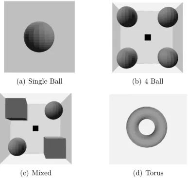
We study the performance of each sampler in different environments shown in Figure 4.5. Figure 4.5(a) has a unit radius ball obstacle at the center of an environ-ment whose bounding box is 8×8×8. Figure 4.5(b) has four unit balls placed on a

(46)

grid in a bounding box that is 8×8×8. Figure 4.5(c) is a variant of Figure 4.5(b). It has a mixture of two unit balls and two cubes which are 2×2×2. Figure 4.5(d) has a torus as the concave obstacle. The robot is a small cube for all environments.

(a) Single Ball (b) 4 Ball

(c) Mixed (d) Torus

Figure 4.5: Four environments are used to compare the distribution of samples pro-duced by UOBPRM and other sampling methods. The robot is a small cube.

We first study the configuration distribution obtained by each method. In Fig-ure 4.5(a), 4.5(b), and 4.5(c), we generate 4000 configurations with each sampling method and compute the node distribution by counting the number of configurations generated in each cell of a regular grid covering the environment by partitioning the space into 16 same sized cells. If the nodes are uniformly distributed, then the num-ber of nodes should be proportional to the surface area for every region. In the torus environment (Figure 4.5(d)), we generate 4000 configurations and find the closest obstacle component each configuration belongs to. The obstacle is modeled as a

(47)

polyhedra composed of triangles. If the nodes are uniformly distributed, the number of configurations will be proportional to the area of the triangle.

4.3.2.1 A Single Ball Environment

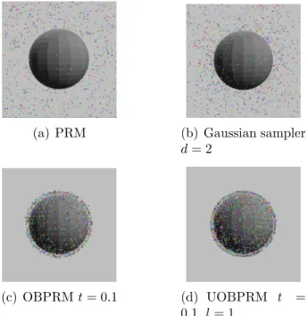
The grid equally partitions the space into 16 cells. Starting from 1, the cells are indexed from left to right from top to bottom. Since the ball symmetrically occupies the center four cells (numbered 6, 7, 10, and 11), a similar number of configurations in these four cells is expected if the distribution is uniform around obstacle surfaces. The configurations generated by PRM are dispersed throughout the environment, as shown in Figure 4.6(a). Figure 4.6(b) shows that Gaussian sampling still generates some configurations quite distant from the obstacle surfaces. Figure 4.6(c) shows the configurations generated by OBPRM with step size t = 0.1 and Figure 4.6(d) is for UOBPRM with step size t = 0.1 and line segment length l = 1. UOBPRM gives a more uniform distribution, and the configurations are closer to the obstacle surfaces compared to other sampling methods (see Figure 4.6).

Figure 4.7 compares the node distribution among different sampling methods. The red bars in Figure 4.7 show the percentage of configurations in the regions occupied by the ball and the blue bars represent the free space. If the configurations are uniformly distributed around obstacle surfaces, each red bar should result in 25% and the blue bar is 0%. OBPRM and UOBPRM are able to generate configurations near obstacles but PRM, Gaussian sampling, and Bridge Test sampling still have configurations scattered in the free space, especially PRM. Table 4.1 shows how the configuration distribution around ball and free space are for each sampling method. UOBPRM has the most uniformly distributed configurations among all sampling methods since its average is ideal and its standard deviation is the lowest. PRM, Gaussian PRM, and Bridge Test PRM still have some configurations distributed in

(48)

(a) PRM (b) Gaussian sampler

d_{= 2}

(c) OBPRMt_{= 0}.₁ _{(d) UOBPRM} t ₌

0._1,l_{= 1}

Figure 4.6: Sample distribution example in the single ball environment. UOBPRM has the most uniformly distributed samples around the obstacle surfaces.

the free space.

Table 4.1: Average and standard deviation of ball and free space in single ball environment for different samplers. The ideal average for ball is 0.25 and free is 0. Error is calculated as the % difference to ideal.

Sampler Ball Free

Avg Std Error Avg Std Error

PRM 0.0629 0.0079 -0.7484 0.0624 0.0071 n/a Gaussian, d = 0.2 0.2328 0.0086 -0.0688 0.0057 0.0093 n/a Bridge Test,d= 3 0.0411 0.0090 -0.8356 0.0696 0.0090 n/a OBPRM 0.2500 0.0093 0.0000 0.0000 0.0000 0.0000 UOBPRM,l = 1 0.2500 0.0089 0.0000 0.0000 0.0000 0.0000

(49)

Figure 4.7: Distribution comparison of ball (red) and free (blue) regions in the single ball environment. Ideal percentage for ball is 25% and free is 0%.

4.3.2.2 Environment With 4 Balls of Equal Size

Here the step size t is 0.1 and the line segment length l is 1. Since we equally partition the space and the obstacle, we have a total of 16 cells with the same obstacle surface area. Ideally, a uniformly distributed obstacle-based sampler will generate same amount of the configurations in each cell.

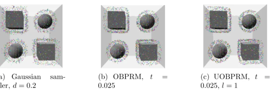
Figure 4.8(a), 4.8(b), and 4.8(c) show the samples generated by Gaussian sam-pler, OBPRM and UOBPRM, respectively. Here UOBPRM and Gaussian sampling produce a distribution that is closer to uniform distribution than other sampling methods. As shown in Figure 4.8(b) and 4.8(c), OBPRM has fewer nodes on the boundary side than it should for a uniform distribution.

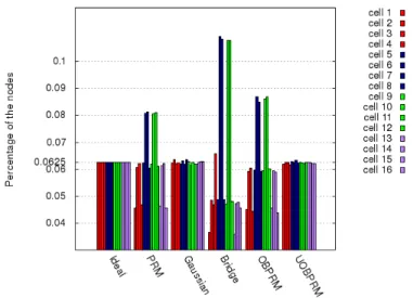
Figure 4.9 shows the node distribution comparison. Each color represents a dif-ferent ball obstacle. If the distribution is uniform, each region will have 6.25% of the nodes. Table 4.2 shows how the configurations are distributed around each ball ob-stacle for various sampling methods. UOBPRM has the most uniformly distributed

(50)

(a) Gaussian sam-pler, d_{= 0}.₂

(b) OBPRM,t_{= 0}.₁ _{(c) UOBPRM,} t ₌

0._1,l_{= 1}

Figure 4.8: Sample distribution example in the 4 balls environment.

configurations comparing to other methods due to its lowest standard deviation.

Figure 4.9: Distribution comparison in the environment with 4 balls of equal size, each ball is a different color. Ideal percentage is 6.25%. UOBPRM and Gaussian sampling generate more uniformly distributed samples than the others.

4.3.2.3 Environment With a Mixture of Balls and Cubes

The step size t here is 0.025 and the line segment length l is 1. After generating 4000 nodes, we separate the environment into four regions where one region contains

(51)

Table 4.2: Average and standard deviation of each ball obstacle in the environment with 4 balls of equal size for different samplers. The ideal average for ball is 0.25. Error is calculated as the % difference to ideal.

Sampler Ball 1 Ball 2 Ball 3 Ball 4

Avg Std Error Avg Std Error Avg Std Error Avg Std Error PRM 0.2151 0.0128 -0.1396 0.2848 0.0125 0.2500 0.2848 0.0126 0.2500 0.2153 0.0128 -0.1388 Gaussian, d = 0.2 0.2505 0.0029 0.0020 0.2503 0.0030 0.0012 0.2488 0.0032 -0.0048 0.2504 0.0034 0.0016 Bridge Test, d= 3 0.1975 0.0526 -0.2100 0.3152 0.0524 -0.2608 0.3107 0.0526 0.2428 0.1765 0.0523 -0.2940 OBPRM 0.2089 0.0153 -0.1644 0.2907 0.0150 0.1628 0.2925 0.0148 0.1700 0.2078 0.0156 -0.1688 UOBPRM,l = 1 0.2488 0.0038 -0.0048 0.2511 0.0034 0.0044 0.2495 0.0039 -0.0020 0.2494 0.0033 -0.0024 36

(52)

one obstacle, either a ball or a cube. The node distribution should be proportional to the obstacle surface area if the nodes are uniformly distributed around obstacle. The surf