What s the Difference? Efficient Set Reconciliation without Prior Context

(1)

What’s the Difference?

Efficient Set Reconciliation without Prior Context

David Eppstein

1

_{Michael T. Goodrich}

1

_{Frank Uyeda}

2

_{George Varghese}

2,3

1_{U.C. Irvine} 2_{U.C. San Diego} 3_{Yahoo! Research}

ABSTRACT

We describe a synopsis structure, the Difference Digest, that allows two nodes to compute the elements belonging to the set difference in a single round with communication overhead proportional to the

size of the differencetimes the logarithm of the keyspace. While set reconciliation can be done efficiently using logs, logs require overhead for every update and scale poorly when multiple users are to be reconciled. By contrast, our abstraction assumes no prior context and is useful in networking and distributed systems appli-cations such as trading blocks in a peer-to-peer network, and syn-chronizing link-state databases after a partition.

Our basic set-reconciliation method has a similarity with the peeling algorithm used in Tornado codes [6], which is not surpris-ing, as there is an intimate connection between set difference and coding. Beyond set reconciliation, an essential component in our Difference Digest is a new estimator for the size of the set ence that outperforms min-wise sketches [3] for small set differ-ences.

Our experiments show that the Difference Digest is more effi-cient than prior approaches such as Approximate Reconciliation Trees [5] and Characteristic Polynomial Interpolation [17]. We use Difference Digests to implement a generic KeyDiff service in Linux that runs over TCP and returns the sets of keys that differ between machines.

Categories and Subject Descriptors

C.2.2 [Computer-Communication Networks]: Network Proto-cols; E.4 [Coding and Information Theory]:

General Terms

Algorithms, Design, Experimentation

1. INTRODUCTION

Two common tasks in networking and distributed systems are

reconciliationanddeduplication. In reconciliation, two hosts each have a set of keys and each seeks to obtain the union of the two sets. The sets could be file blocks in a Peer-to-Peer (P2P) system or link

Permission to make digital or hard copies of all or part of this work for personal or classroom use is granted without fee provided that copies are not made or distributed for profit or commercial advantage and that copies bear this notice and the full citation on the first page. To copy otherwise, to republish, to post on servers or to redistribute to lists, requires prior specific permission and/or a fee.

state packet identifiers in a routing protocol. In deduplication, on the other hand, two hosts each have a set of keys, and the task is to identify the keys in the intersection so that duplicate data can be deleted and replaced by pointers [16]. Deduplication is a thriving industry: for example, Data Domain [1, 21] pioneered the use of deduplication to improve the efficiency of backups.

Both reconciliation and deduplication can be abstracted as the problem of efficiently computing theset difference between two sets stored at two nodes across a communication link. The set dif-ference is the set of keys that are in one set but not the other. In reconciliation, the difference is used to compute the set union; in deduplication, it is used to compute the intersection. Efficiency is measured primarily by the bandwidth used (important when the two nodes are connected by a wide-area or mobile link), the latency in round-trip delays, and the computation used at the two hosts. We are particularly interested in optimizing the case when the set dif-ference is small (e.g., the two nodes have almost the same set of routing updates to reconcile, or the two nodes have a large amount of duplicate data blocks) and when there is no prior communication or context between the two nodes.

For example, suppose two users, each with a large collection of songs on their phones, meet and wish to synchronize their libraries. They could do so by exchanging lists of all of their songs; however, the amount of data transferred would be proportional to the total number of songs they have rather than the size of the difference. An often-used alternative is to maintain a time-stamped log of updates together with a record of the time that the users last communicated. When they communicate again,Acan sendB all of the updates since their last communication, and vice versa. Fundamentally, the use of logs requires prior context, which we seek to avoid.

Logs have more specific disadvantages as well. First, the log-ging system must be integrated with any system that can change user data, potentially requiring system design changes. Second, if reconciliation events are rare, the added overhead to update a log each time user data changes may not be justified. This is partic-ularly problematic for "hot" data items that are written often and may be in the log multiple times. While this redundancy can be avoided using a hash table, this requires further overhead. Third, a log has to be maintained for every other user this user may wish to synchronize with. Further, two usersAandBmay have received the same update from a third userC, leading to redundant commu-nication. Multi-party synchronization is common in P2P systems and in cases where users have multiple data repositories, such as their phone, their desktop, and in the cloud. Finally, logs require stable storage and synchronized time which are often unavailable on networking devices such as routers.

To solve the set-difference problem efficiently without the use of logs or other prior context, we devise a data structure called a

(2)

Difference Digest, which computes the set difference with com-munication proportional to the size of the difference between the sets being compared. We implement and evaluate a simple key-synchronization service based on Difference Digests and suggest how it can improve the performance in several contexts. Settings in which Difference Digests may be applied include:

• Peer-to-peer:PeerAandBmay receive blocks of a file from other peers and may wish to receive only missing blocks from each other.

• Partition healing:When a link-state network partitions, routers in each partition may each obtain some new link-state pack-ets. When the partition heals by a link joining routerAand B, bothA andB only want to exchange new or changed link-state packets.

• Deduplication:If backups are done in the cloud, when a new file is written, the system should only transmit the chunks of the file that are not already in the cloud.

• Synchronizing parallel activations:A search engine may use two independent crawlers with different techniques to har-vest URLs but they may have very few URLs that are dif-ferent. In general, this situation arises when multiple actors in a distributed system are performing similar functions for efficiency or redundancy.

• Opportunistic ad hoc networks: These are often character-ized by low bandwidth and intermittent connectivity to other peers. Examples include rescue situations and military vehi-cles that wish to synchronize data when they are in range. The main contributions of the paper are as follows:

• IBF Subtraction:The first component of the Difference Di-gest is an Invertible Bloom Filter or IBF [9, 13]. IBF’s were previously used [9] for straggler detection at a single node, to identify items that were inserted and not removed in a stream. We adapt Invertible Bloom Filters for set reconciliation by defining a new subtraction operator on whole IBF’s, as op-posed to individual item removal.

• Strata Estimator: Invertible Bloom Filters need to be sized appropriately to be efficiently used for set differences. Thus a second crucial component of the Difference Digest is a new Strata Estimator method for estimating thesize of the differ-ence. We show that this estimator is much more accurate for small set differences (as is common in the final stages of a file dissemination in a P2P network) than Min-Wise Sketches [3, 4] or random projections [14]. Besides being an integral part of the Difference Digest, our Strata Estimator can be used independently to find, for example, which of many peers is most likely to have a missing block.

• KeyDiff Prototype:We describe a Linux prototype of a generic KeyDiff service based on Difference Digests that applica-tions can use to synchronize objects of any kind.

• Performance Characterization: The overall system perfor-mance of Difference Digests is sensitive to many parame-ters, such as the size of the difference, the bandwidth avail-able compared to the computation, and the ability to do pre-computation. We characterize the parameter regimes in which Difference Digests outperform earlier approaches, such as MinWise hashes, Characteristic Polynomial Interpolation [17], and Approximate Reconciliation Trees [5].

Going forward, we discuss related work in Section 2. We present our algorithms and analysis for the Invertible Bloom Filter and Strata Estimator in Sections 3 & 4. We describe our KeyDiff proto-type in Section 5, evaluate our structures in Section 6 and conclude in Section 7.

2. MODEL AND RELATED WORK

We start with a simple model of set reconciliation. For two sets SA, SB each containing elements from a universe, U = [0, u),

we want to compute the set difference,DA−BandDB−A, where

DA−B = SA−SB such that for alls ∈ DA−B, s ∈ SAand

s /∈SB. Likewise,DB−A=SB−SA. We say thatD=DA−B∪

DB−Aandd =|D|. Note that sinceDA−B∩DB−A =∅,d=

|DA−B|+|DB−A|. We assume thatSA and SB are stored at

two distinct hosts and attempt to compute the set difference with minimal communication, computation, storage, and latency.

Several prior algorithms for computing set differences have been proposed. The simplest consists of hosts exchanging lists, each containing the identifiers for all elements in their sets, then scan-ning the lists to remove common elements. This requires O(|SA|+

|SB|) communication and O(|SA| × |SB|) time. The run time can

be improved to O(|SA|+|SB|) by inserting one list into a hash

table, then querying the table with the elements of the second list. The communication overhead can be reduced by a constant fac-tor by exchanging Bloom filters [2] containing the elements of each list. Once in possession of the remote Bloom Filter, each host can query the filter to identify which elements are common. Funda-mentally, a Bloom Filter still requires communication proportional to the size of the sets (and not the difference) and incurs the risk of false positives. The time cost for this procedure is O(|SA|+|SB|).

The Bloom filter approach was extended using Approximate Rec-onciliation Trees [5], which requires O(dlog(|SB|)) recovery time,

and O(|SB|) space. However, givenSAand an Approximate

Rec-onciliation Tree forSB, a host can only computeDA−B, i.e., the

elements unique toSA.

An exact approach to the set-difference problem was proposed by Minksyet al. [17]. In this approach, each set is encoded us-ing a linear transformation similar to Reed-Solomon codus-ing. This approach has the advantage of O(d) communication overhead, but requires O(d3_{) time to decode the difference using Gaussian}

elim-ination; asymptotically faster decoding algorithms are known, but their practicality remains unclear. Additionally, whereas our Strata Estimator gives an accurate one-shot estimate of the size of the dif-ference prior to encoding the difdif-ference itself, Minskyet al.use an iterative doubling protocol for estimating the size of the difference, with a non-constant number of rounds of communication. Both the decoding time and the number of communication rounds (latency) of their system are unfavorable compared to ours.

Estimating Set-Difference Size. A critical sub-problem is an initial estimation of the size of the set difference. This can be esti-mated with constant overhead by comparing a random sample [14] from each set, but accuracy quickly deteriorates when thedis small relative to the size of the sets.

Min-wise sketches [3, 4] can be used to estimate the set similar-ity (r= |SA∩SB|

|SA∪SB|). Min-wise sketches work by selectingkrandom hash functionsπ1, . . . , πkwhich permute elements withinU. Let

min(πi(S))be the smallest value produced byπiwhen run on the

elements ofS. Then, a Min-wise sketch consists of thekvalues min(π1(S)), . . . , min(πk(S)). For two Min-wise sketches,MA

andMB, containing the elements ofSAandSB, respectively, the

set similarity is estimated by the of number of hash function return-ing the same minimum value. IfSAandSBhave a set-similarityr,

(3)

will bem=rk. Inversely, given thatmcells ofMAandMBdo

match, we can estimate thatr = m

k. Given the set-similarity, we

can estimate the difference asd=1_1+r−r(|SA|+|SB|).

As with random sampling, the accuracy of the Min-wise esti-mator diminishes for smaller values ofkand for relatively small set differences. Similarly, Cormodeet al.[8] provide a method for dynamic sampling from a data stream to estimate set sizes using a hierarchy of samples, which include summations and counts. Like-wise, Cormode and Muthukrishnan [7] and Schwelleret al.[20] describe sketch-based methods for finding large differences in traf-fic flows. (See also [19].)

An alternative approach to estimating set-difference size is pro-vided by [11], whose algorithm can more generally estimate the difference between two functions with communication complex-ity very similar to our Strata Estimator. As with our results, their method has a small multiplicative error even when the difference is small. However, it uses algebraic computations over finite fields, whereas ours involves only simple, and more practical, hashing-based data structures.

While efficiency of set difference estimation for small differ-ences may seem like a minor theoretical detail, it can be important in many contexts. Consider, for instance, the endgame of a P2P file transfer. Imagine that a BitTorrent node has 100 peers, and is miss-ing only the last block of a file. Min-wise or random samples from the 100 peers will not identify the right peer if all peers also have nearly finished downloading (small set difference). On the other hand, sending a Bloom Filter takes bandwidth proportional to the number of blocks in file, which can be large. We describe our new estimator in Section 3.2.

3. ALGORITHMS

In this section, we describe the two components of the Differ-ence Digest: an Invertible Bloom Filter (IBF) and a Strata Estima-tor. Our first innovation is taking the existing IBF [9, 13] and in-troducing a subtraction operator in Section 3.1 to computeDA−B

andDB−Ausing a single round of communication of size O(d).

Encoding a setSinto an IBF requires O(|S|) time, but decoding to recoverDA−B andDB−A requires only O(d) time. Our

sec-ond key innovation is a way of composing several sampled IBF’s of fixed size into a new Strata Estimator which can effectively esti-mate the size of the set difference using O(log(|U_|_{)) space.}

3.1 Invertible Bloom Filter

We now describe the Invertible Bloom Filter (IBF), which can si-multaneously calculateDA−BandDB−Ausing O(d) space. This

data structure encodes sets in a fashion that is similar in spirit to Tornado codes’ construction [6], in that it randomly combines ele-ments using the XOR function. We will show later that this simi-larity is not surprising as there is a reduction between set difference and coding across certain channels. For now, note that whereas Tor-nado codes are for a fixed set, IBF’s are dynamic and, as we show, even allow for fast set subtraction operations. Likewise, Tornado codes rely on Reed-Solomon codes to handle possible encoding errors, whereas IBF’s succeed with high probability without rely-ing on an inefficient fallback computation. Finally, our encodrely-ing is much simpler than Tornado codes because we use a simple uniform random graph for encoding while Tornado codes use more complex random graphs with non-uniform degree distributions.

We start with some intuition. An IBF is named because it is sim-ilar to a standard Bloom Filter—except that it can, with the right settings, beinvertedto yield some of the elements that were in-serted. Recall that in a counting Bloom Filter [10], when a key Kis inserted,Kis hashed into several locations of an array and

a count,count, is incremented in each hashed location. Deletion ofKis similar except thatcountis decremented. A check for whetherK exists in the filter returns true if all locations thatK hashes to have non-zerocountvalues.

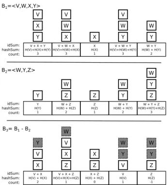
An IBF has another crucial field in each cell (array location) be-sides the count. This is theidSum: the XOR of all key IDs that hash into that cell. Now imagine that two peers, Peer 1 and Peer 2, doing set reconciliation on a large file of a million blocks indepen-dently compute IBF’s,B1andB2, each with 100 cells, by inserting

an ID for each block they possess. Note that a standard Bloom fil-ter would have a size of several million bits to effectively answer whether a particular key is contained in the structure. Observe also that if each ID is hashed to 3 cells, an average of 30,000 keys hash onto each cell. Thus, eachcountwill be large and theidSumin each cell will be the XOR of a large number of IDs. What can we do with such a small number of cells and such a large number of collisions?

Assume that Peer 1 sendsB1to Peer 2, an operation only

requir-ing bandwidth to send around 200 fields (100 cells×2 fields/cell). Peer 2 then proceeds to “subtract” its IBFB2fromB1. It does this

cell by cell, by subtracting thecountand XORing theidSumin the corresponding cells of the two IBF’s.

Intuitively, if the two peers’ blocks sets are almost the same (say, 25 different blocks out of a million blocks), all the common IDs that hash onto the same cell will be cancelled fromidSum, leaving only the sum of the unique IDs (those that belong to one peer and not the other) in theidSumof each cell. This follows assuming that Peer 1 and Peer 2 use the same hash function so that any common element,c, is hashed to the same cells in bothB1andB2. When

we XOR theidSumin these cells,cwill disappear because it is XORed twice.

In essense, randomly hashing keys to, say three, cells, is identical to randomly throwing three balls into the same 100 bins for each of the 25 block ID’s. Further, we will prove that if there are sufficient cells, there is a high probability that at least one cell is “pure” in that it contains only a single element by itself.

A “pure” cell signals its purity by having itscountfield equal to 1, and, in that case, theidSumfield yields the ID of one ele-ment in the set difference. We delete this eleele-ment from all cells it has hashed to in the difference IBF by the appropriate subtractions; this, in turn, may free up more pure elements that it can in turn be decoded, to ultimately yield all the elements in the set difference.

The reader will quickly see subtleties. First, a numericalcount

value of 1 is necessary but not sufficient for purity. For example, if we have a cell in one IBF with two keysX andY and the corre-sponding cell in the second IBF has keyZ, then when we subtract we will get a count of 1, butidSumwill have the XOR ofX, Y andZ. More devious errors can occur if four IDsW, X, Y, Z sat-isfyW+X =Y+Z. To reduce the likelihood of decoding errors to an arbitrarily small value, IBF’s use a third field in each cell as a checksum: the XOR of the hashes of all IDs that hash into a cell, but using a different hash functionHcthan that used to determine

the cell indices. If an element is indeed pure, then the hash sum should beHc(idSum).

A second subtlety occurs if Peer 2 has an element that Peer 1 does not. Could the subtractionB1−B2produce negative values

foridSumandcount? Indeed, it can and the algorithm deals with this: for example, inidSumby using XOR instead of addition and subtraction, and in recognizing purity bycountvalues of 1or-1. While IBF’s were introduced earlier [9, 13], whole IBF subtraction is new to this paper; hence, negative counts did not arise in [9, 13]. Figure 1 summarizes the encoding of a setSand Figure 2 gives a small example of synchronizing the sets at Peer 1 (who has keys

(4)

S = <s1, s2, s3, ... >

...

Hk1 Hk2 Hkk B: idSum += s1 hashSum += Hc(s1) count++ B[j]:

Figure 1: IBF Encode. Hash functions are used to map each element of the set tokcells of the IBF table.

V, W, X andY) and Peer 2 (who has keysW, Y andZ). Each element is hashed into 3 locations: for example,Xis hashed into buckets 1, 2 and 3. WhileX is by itself in bucket 3, after sub-tractionZalso enters, causing thecountfield to (incorrectly) be zero. Fortunately, after subtraction, bucket4becomes pure asV is by itself. Note that bucket5is also pure withZ by itself, and is signaled by a count of -1. Decoding proceeds by first deleting eitherV orZ, and then iterating until no pure cells remain.

Into how many cells should each element be hashed? We refer to this parameter as thehash_count. If the hash_countis too small, say 1, then there will be a high probability of finding pure cells initially, but once a pure element has been recorded and removed there are no other cells from which to remove it. Thus, two or more keys that have been hashed into the same cell cannot be decoded. On the other hand, ifhash_countis too big, it is unlikely that there will be a pure element by itself to begin the process. We will show thathash_countvalues of 3 or 4 work well in practice.

Encode. First, assume that we have an oracle which, givenSA

andSB, returns the size of the set difference,d. We will describe

the construction of such an oracle in Section 3.2. We allocate an IBF, which consists of a tableBwithn=αdcells, whereα≥1. Each cell of the table contains three fields (idSum,hashSumand

count) all initialized to zero.

Additionally, hosts agree on two hash functions,HcandHk, that

map elements inU_{uniformly into the space}_[0_{, h}₎_{, where}_h_≤_u_.

Additionally, they agree on a value,k, called thehash_count

which is the number of times each element is hashed. The algo-rithm for encoding a setSinto an IBF is given in Algorithm 1 and illustrated in Figure 1. For each element inS, we generatek dis-tinct random indices intoB. To do this we recursively callHk()

with an initial input ofsiand take the modulus bynuntilk

dis-tinct indices have been generated. More simply, an implementation could choose to usekindependent hash functions. Regardless, for each indexjreturned, we XORsiintoB[j].idSum, XORHc(si)

intoB[j].hashSum, and incrementB[j].count.

Algorithm 1IBF Encode

forsi∈Sdo

forjin HashToDistinctIndices(si, k, n)do

B[j].idSum=B[j].idSum⊕si

B[j].hashSum=B[j].hashSum⊕Hc(si)

B[j].count=B[j].count+ 1

Subtract.For each indexiin two IBF’s,B1andB2, we subtract

B2[i]fromB1[i]. Subtraction can be done in place by writing the

resulting values back toB1, or non-destructively by writing values

idSum: hashSum: count: Y H(Y) 1 W + Z H(W) + H(Z) 2 Z H(Z) 1 W + Y H(W) + H(Y) 2 W + Y + Z H(W)+H(Y)+H(Z) 3 Y W Z Z W Y W Y Z B2=<W,Y,Z> V + X + Y H(V)+H(X)+H(Y) 3 V + W + X H(V)+H(W)+H(X) 3 X H(X) 1 V + W + Y H(V)+H(W)+H(Y) 3 W + Y H(W) + H(Y) 2 idSum: hashSum: count: V X Y V W X X V W Y W Y B1=<V,W,X,Y> idSum: hashSum: count: V + X H(V) + H(X) 2 V + X + Z H(V)+H(X)+H(Z) 1 X + Z H(X) + H(Z) 0 V H(V) 1 Z H(Z) -1 W Y Z Z Z V X Y V W X X V W Y B3= B1 - B2

Figure 2: IBF Subtract. IBFB3results from subtracting IBF

B2from IBFB1 cell by cell. To subtract cells, theidSumand

hashSumfields are XOR’ed, andcountfields are subtracted.

The elements common toB1 andB2(shown shaded) are

can-celled during the XOR operation.

to a new IBF of the same size. We present a non-destructive version in Algorithm 2. Intuitively, this operation eliminates common ele-ments from the resulting IBF as they cancel from theidSumand

hashSumfields as shown in Figure 2.

Algorithm 2IBF Subtract (B3=B1−B2)

foriin0, . . . , n−1 do

B3[i].idSum=B1[i].idSum⊕B2[i].idSum

B3[i].hashSum=B1[i].hashSum⊕B2[i].hashSum

B3[i].count=B1[i].count-B2[i].count

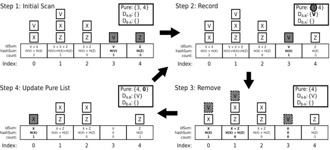
Decode. We have seen that to decode an IBF, we must recover “pure” cells from the IBF’s table. Pure cells are those whoseidSum

matches the value of an elementsin the set difference. In order to verify that a cell is pure, it must satisfy two conditions: thecount

field must be either 1 or -1, and thehashSumfield must equal Hc(idSum). For example, if a cell is pure, then the sign of the

countfield is used to determine which setsis unique to. If the IBF is the result of subtracting the IBF forSB from the IBF for

SA, then a positivecountindicatess∈DA−B, while a negative

count indicatess∈DB−A.

Decoding begins by scanning the table and creating a list of all pure cells. For each pure cell in the list, we add the value s=idSumto the appropriate output set (DA−BorDB−A) and

re-movesfrom the table. The process of removal is similar to that of insertion. We compute the list of distinct indices wheresis present, then decrementcountand XOR theidSumandhashSumbys andHc(s), respectively. If any of these cells becomes pure afters

is removed, we add its index to the list of pure cells.

Decoding continues until no indices remain in the list of pure cells. At this point, if all cells in the table have been cleared (i.e. all

(5)

Algorithm 3IBF Decode (B→DA−B, DB−A) fori= 0ton−1 do ifB[i]is purethen Addito pureList whilepureList6=∅do i=pureList.dequeue()

ifB[i]is not purethen

continue s=B[i].idSum c=B[i].count ifc >0then addstoDA−B else addstoDB−A forjin DistinctIndices(s, k, n)do B[j].idSum=B[j].idSum⊕s B[j].hashSum=B[j].hashSum⊕Hc(s) B[j].count=B[j].count-c fori= 0ton−1 do

ifB[i].idSum6= 0ORB[i].hashSum6= 0B[i].count6= 0

then

return FAIL

return SUCCESS

fields have value equal to zero), then the decoding process has suc-cessfully recovered all elements in the set difference. Otherwise, some number of elements remain encoded in the table, but insuffi-cient information is available to recover them. The pseudocode is given in Algorithm 3 and illustrated in Figure 3.

3.2 Strata Estimator

To use an IBF effectively, we must determine the approximate size of the set difference,d, since approximately1.5dcells are re-quired to successfully decode the IBF. We now show how to es-timatedusingO(log(u))data words, whereuis the size of the universe of set values. If the set difference is large, estimators such as random samples [14] and Min-wise Hashing [3, 4] will work well. However, we desire an estimator that can accurately estimate very small differences (say10) even when the set sizes are large (say million).

Flajolet and Martin (FM) [12] give an elegant way to estimate set sizes (not differences) usinglog(u)bits. Each bitiin the esti-mator is the result of sampling the set with probability1/2i; biti is set to 1, if at least 1 element is sampled when sampling with this probability. Intuitively, if there are24 _{= 16}_{distinct values in the}

set, then when sampling with probability1/16, it is likely that bit 4will be set. Thus the estimator returns2Ias the set size, whereI is the highest strata (i.e., bit) such that bitIis set.

While FM data structures are useful in estimating the size of two sets, they do not help in estimating the size of the difference as they contain no information that can be used to approximate which elements are common. However, we cansample the set difference

using the same technique as FM. Given that IBF’s can compute set differences with small space, we use a hierarchy of IBF’s as strata. Thus PeerAcomputes a logarithmic number of IBF’s (strata), each of some small fixed size, say 80 cells.

Compared to the FM estimator for set sizes, this is very expen-sive. Using 32 strata of 80 cells is around 32 Kbytes but is the only estimator we know that is accurate at very small set differences and yet can handle set difference sizes up to232. In practice, we build a lower overhead composite estimator that eliminates higher strata and replaces them with a MinWise estimator, which is more

accu-rate for large differences. Note that 32 Kbytes is still inexpensive when compared to the overhead of naively sending a million keys.

Proceeding formally, we stratifyU_into_L _{= log(}_u₎_partitions,

P0, . . . , PL, such that the range of theith partition covers1/2i+1

ofU_{. For a set,}_S_{, we encode the elements of}_S_{that fall into}

par-titionPi into theith IBF of the Strata Estimator. PartitioningU

can be easily accomplished by assigning each element to the par-tition corresponding to the number of trailing zeros in its binary representation.

A host then transmits the Strata Estimator for its set to its remote peer. For each IBF in the Strata Estimator, beginning at stratum Land progressing toward stratum0, the receiving host subtracts the corresponding remote IBF from the local IBF, then attempts to decode. For each successful decoding, the host adds the number of recovered elements to a counter. If the pair of IBF’s at indexi fails to decode, then we estimate that the size of the set difference is the value of the counter (the total number of elements recovered) scaled by2i+1_{. We give the pseudocode in Algorithms 4 and 5.}

We originally designed the strata estimator by starting with stra-tum0and finding the first value ofi≥0which decoded success-fully, following the Flajolet-Martin strategy and scaling the amount recovered by2i_{. However, the estimator in the pseudocode is much}

better because it uses information inallstrata that decode success-fully and not just the lowest such strata.

In the description, we assumed that the elements inSAandSB

were uniformly distributed throughoutU_{. If this condition does not}

hold, the partitions formed by counting the number of low-order zero bits may skew the size of our partitions such that strataidoes not hold roughly|S|/2i+1_{. This can be easily solved by choosing}

some hash function,Hz, and inserting each element,s, into the IBF

corresponding to the number of trailing zeros inHz(s).

Algorithm 4Strata Estimator Encode using hash functionHz

fors∈Sdo

i=Number of trailing zeros inHz(s).

Insertsinto thei-th IBF

Algorithm 5Strata Estimator Decode count= 0

fori= log(u)down to−1do

ifi <0or IBF1[i]−IBF2[i]does not decodethen

return 2i+1_×_count

count += number of elements in IBF1[i]−IBF2[i]

The obvious way to combine the Strata Estimator and IBF is to have nodeArequest an estimator from nodeB, use it to estimate d, then request an IBF of sizeO(d). This would taketworounds or at least two round trip delays. A simple trick is to instead have Ainitiate the process by sending its own estimator toB. AfterB receives the Strata Estimator fromA, it estimatesdand replies with an IBF, resulting inoneround to compute the set difference.

4. ANALYSIS

In this section we review and prove theoretical results concerning the efficiency of IBF’s and our stratified sampling scheme.

THEOREM 1. LetSandTbe disjoint sets withdtotal elements, and letB be an invertible Bloom filter withC = (k+ 1)dcells, wherek=hash_{_}count_{is the number of random hash functions in} B, and with at leastΩ(klogd)bits in each hashSum field. Suppose that (starting from a Bloom filter representing the empty set) each

(6)

idSum: hashSum: count: V + X H(V) + H(X) 2 V + X + Z H(V)+H(X)+H(Z) 1 X + Z H(X) + H(Z) 0 V H(V) 1 Z H(Z) -1 Z Z Z V X V X X V Pure: DA-B: DB-A: 0 1 2 3 4 Index: {3, 4} {} {} Step 1: Initial Scan

idSum: hashSum: count: V + X H(V) + H(X) 2 V + X + Z H(V)+H(X)+H(Z) 1 X + Z H(X) + H(Z) 0 V H(V) 1 Z H(Z) -1 Z Z Z V X V X X V Pure: DA-B: DB-A: 0 1 2 3 4 Index: {3, 4} {V} {} Step 2: Record Step 3: Remove idSum: hashSum: count: X H(X) 1 X + Z H(X) + H(Z) 0 X + Z H(X) + H(Z) 0 0 0 0 Z H(Z) -1 Z Z Z V X V X X V Pure: DA-B: DB-A: 0 1 2 3 4 Index: {4} {V} {} Step 4: Update Pure List

idSum: hashSum: count: X H(X) 1 X + Z H(X) + H(Z) 0 X + Z H(X) + H(Z) 0 0 0 0 Z H(Z) -1 Z Z Z X X X Pure: DA-B: DB-A: 0 1 2 3 4 Index: {4, 0} {V} {}

Figure 3: IBF Decode. We first scan the IBF for pure cells and add these indices (3&4) to the Pure list (Step 1). In Step 2, we dequeue the first index from the Pure list, then add the value of theidSumto the appropriate output set (V →DA−B). We then remove V

from the IBF by using thekhash functions to find where it was inserted during encoding and subtracting it from these cells. Finally, if any of these cells have now become pure, we add them to the Pure list (Step 4). We repeat Steps 2 through 4 until no items remain in the Pure list.

item inSis inserted intoB, and each item inT is deleted fromB. Then with probability at mostO(d−k₎_{the IBFDecode operation} will fail to correctly recoverSandT.

PROOF. The proof follows immediately from the previous anal-ysis for invertible Bloom filters (e.g., see [13]).

We also have the following.

COROLLARY 1. LetSandT be two sets having at mostd ele-ments in their symmetric difference, and letBSandBT be invert-ible Bloom filters, both with the parameters as stated in Theorem 1, withBS representing the setS andBT representing the setT. Then with probability at mostO(d−k₎ _{we will fail to recover}_S andT by applying the IBFSubtract operation toBS andBT and then applying the IBFDecode operation to the resulting invertible Bloom filter.

PROOF. DefineS′₌_S₋_T_and_T′₌_T₋_S_{. Then}_S′_and_T′ are disjoint sets of total size at mostd, as needed by Theorem 1.

The corollary implies that in order to decode an IBF that uses 4 independent hash functions with high probability, then one needs an overhead ofk+ 1 = 5. In other words, one has to use5dcells, wheredis the set difference. Our experiments later, however, show that an overhead that is somewhat less than2suffices. This gap is narrowed in [13] leveraging results on finding a 2-core (analogous to a loop) in random hypergraphs.

Let us next consider the accuracy of our stratified size estimator. Suppose that a setShas cardinalitym, and letibe any natural num-ber. Then theith stratum of our strata estimator forShas expected cardinalitym/2i_{. The following lemma shows that our estimators}

will be close to their expectations with high probability.

LEMMA 1. For anys >1, with probability1−2−s, and for allj < i, the cardinality of the union of the strata numberedjor greater is within a multiplicative factor of1±O(p

s2i_/m₎_{of its} expectation.

PROOF. LetYj be the size of the union of strata numberedj

or greater forj = 0,1, . . . , i, and letµj be its expectation, that

is, µj = E(Yj) = m/2j. By standard Chernoff bounds (e.g.,

see [18]), forδ >0, Pr (Yj>(1 +δ)µj)< e−µjδ 2_/4 and Pr (Yj<(1−δ)µj)< e−µjδ 2_/4 . By takingδ=p 4(s+ 2)(2i_/m_{) ln 2}_{, which is}_O₍p s2i_/m₎_{, we}

have that the probability that a particularYjis not within a

multi-plicative factor of1±δof its expectation is at most 2e−µjδ2/4_≤₂−(s+1)2i−j

.

Thus, by a union bound, the probability that anyYjis not within a

multiplicative factor of1±δof its expectation is at most

i X j=0 2−(s+1)2i−j , which is at most2−s_.

Putting these results together, we have the following:

THEOREM 2. Letǫandδbe constants in the interval (0,1), and letS andT be two sets whose symmetric difference has car-dinalityd. If we encode the two sets with our strata estimator, in which each IBF in the estimator hasCcells usingkhash functions, whereCandkare constants depending only onǫandδ, then, with probability at least1−ǫ, it is possible to estimate the size of the set difference within a factor of1±δofd.

PROOF. By the same reasoning as in Corollary 1, each IBF at leveliin the estimator is a valid IBF for a sample of the symmetric difference ofSandTin which each element is sampled with prob-ability1/2i+1_{. By Theorem 1, having each IBF be of}_C_{= (}_k₊₁₎_g

(7)

cells, wherek=⌈log 1/ǫ⌉andg≥2, then we can decode a set of gelements with probability at least1−ǫ/2.

We first consider the case whend≤c2

0δ−2log(1/ǫ), wherec0is

the constant in the big-oh of Lemma 1. That is, the size of the sym-metric difference betweenSandTis at most a constant depending only onǫandδ. In this case, if we take

g= max˘

2,⌈c20δ−2log(1/ǫ)⌉ ¯

andk = ⌈log 1/ǫ⌉, then the level-0 IBF, withC = (k + 1)d cells, will decode its set with probability at least1−ǫ/2, and our estimator will learn the exact set-theoretic difference betweenS andT, without error, with high probability.

Otherwise, let ibe such thatd/2i _≈ _c2

0δ2/log(1/ǫ) and let

g = max˘

2,⌈c20δ−2log(1/ǫ)⌉ ¯

andk = ⌈log 1/ǫ⌉, as above. So, with probability1−ǫ/2, using an IBF ofC= (k+ 1)dcells, we correctly decode the elements in theith stratum, as noted above. By Lemma 1 (withs=⌈log 1/ǫ⌉+ 1), with probability1−ǫ/2, the cardinality of the number of items included in theith and higher strata are within a multiplicative factor of1±δof its expectation. Thus, with high probability, our estimate fordis within a1±δ factor ofd.

Comparison with Coding:Readers familiar with Tornado codes will see a remarkable similarity between the decoding procedure used for Tornado codes and IBF’s. This follows because set recon-ciliation and coding are equivalent. Assume that we have a system-atic code that takes a set of keys belonging to a setSAand codes

it using check wordsC1throughCn. Assume further that the code

can correct for up toderasures and/or insertions. Note that Tornado codes are specified to deal only with erasures not insertions.

Then, to compute set differenceAcould send the check words C1throughCnwithoutsending the "data words" in setSA. When

B receives the check words, B can treat its set SB as the data

words. Then, together with the check words,Bcan computeSA

and hence the set difference. This will work as long asSB has at

mostderasures or insertions with respect to setSA.

Thus any code that can deal with erasures and insertions can be used for set difference, and vice versa. A formal statement of this equivalence can be found in [15]. This equivalence explains why the existing deterministic set difference scheme, CPI, is analogous to Reed-Solomon coding. It also explains why IBF’s are analogous to randomized Tornado codes. While more complicated Tornado-code like constructions could probably be used for set difference, the gain in space would be a small constant factor from say2dto d+ǫ, the increased complexity is not worthwhile because the real gain in set reconciliation is going down fromO(n)toO(d), where nis the size of the original sets.

5. THE KEYDIFF SYSTEM

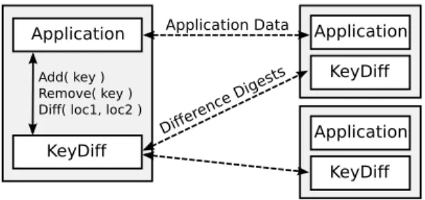
We now describeKeyDiff, a service that allows applications to compute set differences using Difference Digests. As shown in Figure 4, the KeyDiff service provides three operations,add,remove, anddiff. Applications can add and remove keys from an instance of KeyDiff, then query the service to discover the set difference be-tween any two instances of KeyDiff.

Suppose a developer wants to write a file synchronization appli-cation. In this case, the application running at each host would map files to unique keys and add these keys to a local instance of Key-Diff. To synchronize files, the application would first run KeyDiff’s

diffoperation to discover the differences between the set stored locally and the set stored at a remote host. The application can then perform the reverse mapping to identify and transfer the files that differ between the hosts.

KeyDiff Application Application

Add( key ) Remove( key ) Diff( loc1, loc2 )

KeyDiff KeyDiff Application Differen ce Digest s Application Data

Figure 4: KeyDiff computes the set difference between any two instances and returns this information to the application.

The KeyDiff service is implemented using a client-server model and is accessed through an API written in C. When a client re-quests the difference between its local set and the set on a remote host, KeyDiff opens a TCP connection and sends a request contain-ing an estimator. The remote KeyDiff instance runs the estimation algorithm to determine the approximate size of the difference, then replies with an IBF large enough for the client to decode with high-probability. All requests and responses between KeyDiff instances travel over a single TCP connection and thediffoperation com-pletes with only a single round of communication.

KeyDiff provides fasterdiffoperations through the use of pre-computation. Internally, KeyDiff maintains an estimator structure that is statically sized and updated online as keys are added and re-moved. However, computing the IBF requires the approximate size of the difference, a value that is not know until after the estima-tion phase. In scenarios where computaestima-tion is a bottleneck, Key-Diff can be configured to maintain several IBF’s of pre-determined sizes online. After the estimation phase, KeyDiff returns the best pre-computed IBF. Thus, the computational cost of building the IBF can be amortized across all of the calls toaddandremove.

This is reasonable because the cost of incrementally updating the Strata Estimator and a few IBF’s on key update is small (a few microseconds) and should be much smaller than the time for the application to create or store the object corresponding to the key. For example, if the application is a P2P application and is synchro-nizing file blocks, the cost to store a new block on disk will be at least a few milliseconds. We will show in the evaluation that if the IBF’s are precomputed, then the latency ofdiffoperations can be 100’s of microseconds for small set differences.

6. EVALUATION

Our evaluation seeks to provide guidance for configuring and predicting the performance of Difference Digests and the KeyDiff system. We address four questions. First, what are the optimal pa-rameters for an IBF? (Section 6.1). Second, how should one tune the Strata Estimator to balance accuracy and overhead? (Section 6.2). Third, how do IBF’s compare with the existing techniques? (Section 6.3). Finally, for what range of differences are Difference Digests most effective compared to the brute-force solution of sending all the keys? (Section 6.4).

Our evaluation uses aU_{of all 32-bit values. Hence, we}

allo-cate 12 bytes for each IBF cell, with 4 bytes given to eachidSum,

hashSumand countfield. As input, we created pairs of sets

containingkeysfromU_{. The keys in the first set,}_S_A_{, were chosen}

randomly without replacement. We then chose a random subset of SAand copied it to the second set,SB. We exercised two degrees

of freedom in creating our input sets: the number of keys inSA,

and the size of the difference betweenSAandSB, which we refer

(8)

0 20 40 60 80 100 0 5 10 15 20 25 30 35 40 45 50

Percent Successfully Decoded

Set Difference 100 keys 1K keys 10K keys 100K keys 1M keys

Figure 5: Rate of successful IBF decoding with 50 cells and 4 hash functions. The ability to decode an IBF scales with the size of the set difference, not the size of the sets.

file pairs. As our objective is set reconciliation, we consider an ex-periment successful only if we are able to successfully determine all of the elements in the set difference.

6.1 Tuning the IBF

We start by verifying that IBF size scales with the size of the set difference and not the total set size. To do so, we generated sets with 100, 1K, 10K, 100K and 1M keys, and deltas between 0 and 50. We then compute the set difference using an IBF with 50 cells. Figure 5 shows the success rate for recovering the entire set dif-ference. We see that for deltas up to 25, the IBF decodes completely with extremely high probability, regardless of set size. At deltas of 45 and 50 the collision rate is so high that no IBF’s are able to completely decode. The results in Figure 5 confirm that decoding success is independent of the original set sizes.

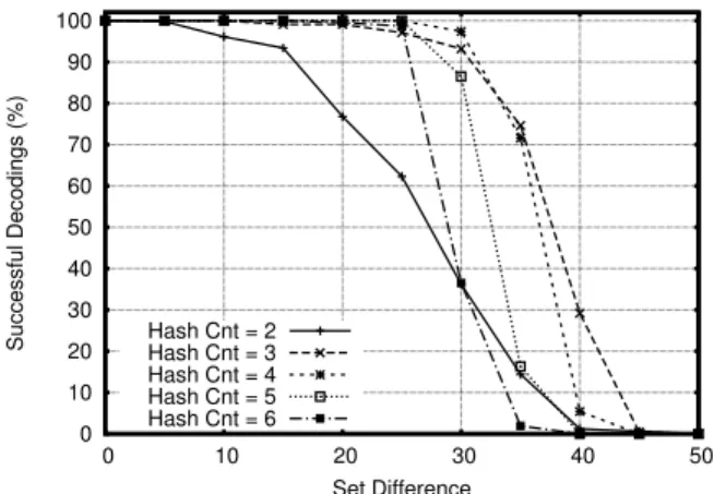
Determining IBF size and number of hash functions. Both the number of IBF cells andhash_count(the number of times an element is hashed) are critical in determining the rate of successful decoding. To evaluate the effect ofhash_count, we attempted to decode sets with 100 keys and deltas between 0 and 50 using an IBF with 50 cells andhash_count’s between 2 and 6. Since the size of the sets does not influence decoding success, these results are representative for arbitrarily large sets. We ran this configuration for 1000 pairs of sets and display our results in Figure 6.

For deltas less than 30,hash_count= 4 decodes 100% of the time, while higher and lower values show degraded success rates. Intuitively, lower hash counts do not provide equivalent decode rates since processing each pure cell only removes a key from a small number of other cells, limiting the number of new pure cells that may be discovered. Higher values ofhash_countavoid this problem but may also decrease the odds that there will initially be a pure cell in the IBF. For deltas greater than 30,hash_count

= 3 provides the highest rate of successful decoding. However, at smaller deltas, 3 hash functions are less reliable than 4, with ap-proximately 98% success for deltas from 15 to 25 and 92% at 30.

To avoid failed decodings, we must allocate IBF’s with more thandcells. We determine appropriate memory overheads (ratio of IBF’s cells to set-difference size) by using sets containing 100K el-ements and varying the number of cells in each IBF as a proportion of the delta. We then compute the memory overhead required for 99% of the IBF’s to successfully decode and plot this in Figure 7.

Deltas below 200 all require at least 50% overhead to completely

0 10 20 30 40 50 60 70 80 90 100 0 10 20 30 40 50 Successful Decodings (%) Set Difference Hash Cnt = 2 Hash Cnt = 3 Hash Cnt = 4 Hash Cnt = 5 Hash Cnt = 6

Figure 6: Probability of successful decoding for IBF’s with 50 cells for different deltas. We vary the number of hashes used to assign elements to cells (hash_count) from 2 to 6.

1 1.2 1.4 1.6 1.8 2 2.2 2.4 10 100 1000 10000 100000 Space Overhead Set Difference Hash Cnt = 3 Hash Cnt = 4 Hash Cnt = 5 Hash Cnt = 6

Figure 7: We evaluate sets containing 100K elements and plot the minimum space overhead (IBF cells/delta) required to com-pletely recover the set difference with 99% certainty.

decode. However, beyond deltas of 1000, the memory overhead reaches an asymptote. As before, we see ahash_countof 4 de-codes consistently with less overhead than 5 or 6, but interestingly,

hash_count= 3 has the lowest memory overhead at all deltas

greater than 200.

6.2 Tuning the Strata Estimator

To efficiently size our IBF, the Strata Estimator provides an es-timate ford. If the Strata Estimator over-estimates, the subsequent IBF will be unnecessarily large and waste bandwidth. However, if the Strata Estimator under-estimates, then the subsequent IBF may not decode and cost an expensive transmission of a larger IBF. To prevent this, the values returned by the estimator should be scaled up so that under-estimation rarely occurs.

In Figure 8, we report the scaling overhead required for var-ious strata sizes such that 99% of the estimates will be greater than or equal to the true difference. Based on our findings from Section 6.1, we focus on Strata Estimators whose fixed-size IBF’s use ahash_countof 4. We see that the scaling overhead drops sharply as the number of cells per IBF is increased from 10 to 40, and reaches a point of diminishing returns after 80 cells. With 80 cells per stratum, any estimate returned by a Strata Estimator

(9)

1 1.5 2 2.5 3 3.5 20 40 60 80 100 120 140 160 Correction Overhead

IBF Size (in cells)

Delta = 10 Delta = 100 Delta = 1000 Delta = 10000 Delta = 100000

Figure 8: Correction overhead needed by the Strata Estimator to ensure that 99% of the estimates are greater than or equal to the true value ofdwhen using strata IBF’s of various sizes.

should be scaled by a factor of 1.39 to ensure that it will be greater than or equal tod99% of the time.

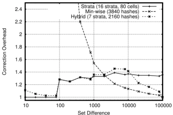
Strata Estimator vs. Min-wise. We next compare our Strata Estimator to the Min-wise Estimator [3, 4] (see Section 2). For our comparison we used sets with 100K elements and deltas ranging from 10 to 100K. Given knowledge of the approximate total set sizes a priori, the number of strata in the Strata estimator can be adjusted to conserve communication costs by only including parti-tions that are likely to contain elements from the difference. Thus, we choose the number of strata to be⌊log2(dmax)⌋, wheredmax

is the largest possible difference. Since our largest delta is 100K, we configure our estimator with 16 strata, each containing 80 cells per IBF. At 12 bytes per IBF cell, this configuration requires ap-proximately 15.3 KB of space. Alternatively, one could allocate a Min-wise estimator with 3840 4-byte hashes in the same space.

In Figure 9, we compare the scaling overhead required such that 99% of the estimates from Strata and Min-wise estimators of the same size are greater than or equal to the true delta. We see that the overhead required by Min-wise diminishes from 1.35 to 1.0 for deltas beyond 2000. Strata requires correction between 1.33 to 1.39 for the same range. However, the accuracy of the Min-wise estimator deteriorates rapidly for smaller delta values. In fact, for all deltas below 200, the 1st percentile of Min-wise estimates are 0, resulting in infinite overhead. Min-wise’s inaccuracy for small deltas is expected as few elements from the difference will be in-cluded in the estimator as the size of the difference shrinks. This makes Min-wise very sensitive to any variance in the sampling pro-cess, leading to large estimation errors. In contrast, we see that the Strata Estimator provides reasonable estimates for all delta values and is particularly good at small deltas, where scaling overheads range between 1.0 and 1.33.

Hybrid Estimator.The Strata Estimator outperforms Min-wise for small differences, while the opposite occurs for large differ-ences. This suggests the creation of a hybrid estimator that keeps the lower strata to accurately estimate small deltas, while augment-ing more selective strata with a saugment-ingle Min-wise estimator. We par-tition our set as before, but if a strata does not exist for a parpar-tition, we insert its elements into the Min-wise estimator. Estimates are performed by summing strata as before, but also by including the number of differences that Min-wise estimates to be in its partition. For our previous Strata configuration of 80 cells per IBF, each strata consumes 960 bytes. Therefore, we can trade a strata for 240

1 1.2 1.4 1.6 1.8 2 2.2 2.4 10 100 1000 10000 100000 Correction Overhead Set Difference

Strata (16 strata, 80 cells) Min-wise (3840 hashes) Hybrid (7 strata, 2160 hashes)

Figure 9: Comparison of estimators when constrained to 15.3 KB. We show the scaling overhead to ensure that 99% of esti-mates are greater than or equal to the true delta.

additional Min-wise hashes. From Figure 9 we see that the Strata Estimator performs better for deltas under 2000. Thus, we would like to keep at most⌊log₂(2000)⌋ = 10strata. Since we expect the most selective strata to contain few elements for a difference of 2000, we are better served by eliminating them and giving more space to Min-wise. Hence, we retain 7 strata, and use the remaining 8640 bytes to allocate a Min-wise estimator with 2160 hashes.

Results from our Hybrid Estimator are plotted in Figure 9 with the results from the Strata and Min-wise estimators. We see that the Hybrid Estimator closely follows the results of the Strata Esti-mator for all deltas up to 2000, as desired. For deltas greater than 2000, the influence of errors from both Strata and Min-wise cause the scaling overhead of the Hybrid estimator to drift up to 1.45 (versus 1.39% for Strata), before it progressively improves in ac-curacy, with perfect precision at 100K. While the Hybrid Estimator slightly increase our scaling overhead from 1.39 to 1.45 (4.3%), it also provides improved accuracy at deltas larger than 10% where over-estimation errors can cause large increases in total data sent.

Difference Digest Configuration Guideline.By using the Hy-brid Estimator in the first phase, we achieve an estimate greater than or equal to the true difference size 99% of the time by scaling the result by 1.45. In the second phase, we further scale by 1.25 to 2.3 and sethash_countto either 3 or 4 depending on the estimate from phase one. In practice, a simple rule of thumb is to construct an IBF in Phase 2 with twice the number of cells as the estimated difference to account for both under-estimation and IBF decoding overheads. For estimates greater than 200, 3 hashes should be used and 4 hashes otherwise.

6.3 Difference Digest vs. Prior Work

We now compare Difference Digests to Approximate Recon-ciliation Trees (ART) [5], Characteristic Polynomial Interpolation (CPISync) [17], and simply trading a sorted list of keys (List). We note thatART’s were originally designed to computemost but not allthe keys inSA −SB. To address this, the system built

in [5] used erasure coding techniques to ensure that hosts received pertinent data. While this approach is reasonable for some P2P applications it may not be applicable to or desirable for all applica-tions described in Section 1. In contrast,CPISyncandListare always able to recover the set difference.

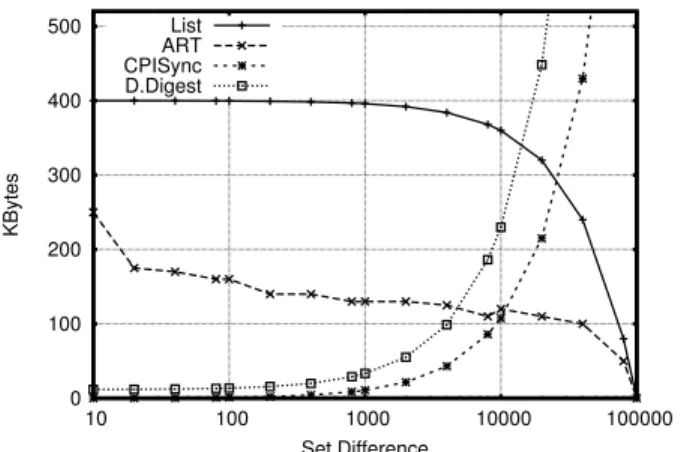
Figure 10 shows the data overhead required by the four algo-rithms. Given that ART’s were not designed for computing the

(10)

0 100 200 300 400 500 10 100 1000 10000 100000 KBytes Set Difference List ART CPISync D.Digest

Figure 10: Data transmission required to reconcile sets with 100K elements. We show the space needed byARTand Differ-ence Digests to recover 95% and 100% of the set differDiffer-ence, respectively, with 99% reliability.

complete set difference, we arbitrarily choose the standard of 95% of the difference 99% of the time and plot the amount of data re-quired to achieve this level of performance withART. ForCPISync, we show the data overhead needed to recover the set difference. In practice, the basic algorithm must be run with knowledge of the difference size, or an interactive approach must be used at greater computation and latency costs. Hence, we show the best case over-head forCPISync. Finally, we plot the data used by Difference Digest for both estimation and reconciliation to compute the com-plete difference 99% of the time.

The results show that the bandwidth required byListandART

decreases as the size of the difference increases. This is intuitive since bothListand theARTencode the contents ofSB, which

is diminishing in size as the size of the difference grows (|SB|=

|SA| − |D|). However,ARToutperformsListsince its compact

representation requires fewer bits to capture the nodes inB. While the size of the Hybrid Estimator stays constant, the IBF grows at an average rate of 24 Bytes (three 4-byte values and a factor of 2 inflation for accurate decoding) per key in the differ-ence. We see that while Difference Digests andCPISynchave the same asymptotic communication complexity,CPISyncrequires less memory in practice at approximately 10 bytes per element in the difference.

Algorithm Selection Guidelines.The results show that for small differences, Difference Digests andCPISyncrequire an order of magnitude less bandwidth thatARTand are better up to a differ-ence of 4,000 (4%) and 10,000 (10%), respectively. However, the fact thatARTuses less space for large deltas is misleading since we have allowedARTto decode only 95% of the difference.CPISync

provides the lowest bandwidth overhead and decodes deterministi-cally, making it a good choice when differences are small and band-width is precious. However, as we discuss next, its computational overhead is substantial.

6.4 KeyDiff Performance

We now examine the benefits of Difference Digest in system-level benchmarks using KeyDiff service described in Section 5. We quantify the performance of KeyDiff using Difference Digests versusART, CPISync, and List. For these experiments, we deployed KeyDiff on two dual-processor quad-core Xeon servers

running Linux 2.6.32.8. Our test machines were connected via 10 Gbps Ethernet and report an average RTT of 93µs.

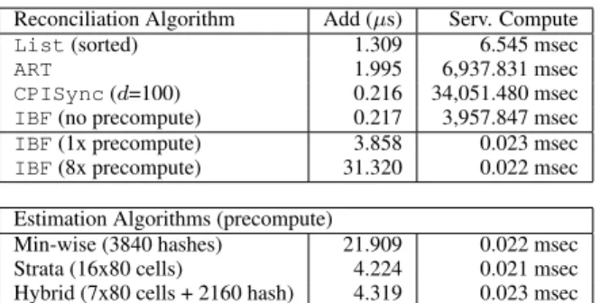
Computational Overhead.In the KeyDiff model, the applica-tions at the client and server both add keys to KeyDiff. Whendiff

is called the client requests the appropriate data from the server to compute the set difference. We begin by evaluating the computa-tion time required to add new keys to KeyDiff and the time required by the server to generate its response when using each algorithm. For this experiment, we added 1 million keys to the KeyDiff server then requested a structure to decode a difference of 100. In Table 1, we show the average time required for these operations.

For adding new keys, we see thatListandARTare slower than bothCPISyncandIBFsince both perform log(|S|)operations — theListto do an ordered insertion, andARTto update hashes along a path in its tree. In contrast,CPISyncandIBFsimply store the new keys to an unordered list until they learn the size of the structure to build from the client’s request.

For server compute time, we note that the latencies correspond closely with the number of memory locations each algorithm touches.

Listis quickest at 6.545 msec, as the server only needs to read and serialize the keys. In contrast,IBFandCPISyncmust allo-cate and populate appropriately-sized structures by scanning their stored lists of keys. ForIBFthis requires updating 4 cells per key, whileCPISyncmust evaluate 100 linear equations, each involv-ing all 1M keys. The time forARTis roughly twice that ofIBF

as it must traverse its tree containing2|S|nodes, to build a Bloom Filter representation of its set.

At the bottom of Table 1, we show theaddand server-compute times for the three estimation algorithms. Note that since the length of the IBF’s in the Strata and Hybrid estimators are static, they can be updated online. We also note that although the Hybrid estimator maintains 2160 Min-wise hash values, its addition times are sig-nificantly lower that the original Min-wise estimator. This occurs because the Min-wise structure in the Hybrid estimator only sam-ples the elements not assigned to one of the seven strata. Thus, while the basic Min-wise estimator must compute 3840 hashes for each key, the Hybrid Min-wise estimator only computes hashes for approximately1/28 _{of the elements in the set. Since each of the}

estimators is updated during itsadd operations, minimal server compute time is required to serialize each structure.

Costs and Benefits of Incremental Updates.As we have seen in Table 1, the server computation time for many of the reconcilia-tion algorithms is significant and will negatively affect the speed of ourdiffoperation. The main challenge forIBFandCPISync

is that the size of the difference must be known before a space-efficient structure can be constructed. We can avoid this runtime computation by maintaining several IBF’s of predetermined sizes within KeyDiff. Each key is added to all IBF’s and, once the size of the difference is know, the smallest suitable IBF is returned. The number of IBF’s to maintain in parallel will depend on the comput-ing and bandwidth overheads encountered for each application.

In Table 1, we see that the time to add a new key when doing pre-computation on 8 IBF’s takes 31µs, two orders of magnitude longer than IBF without precomputation. However, this reduces the server compute time to from 3.9 seconds to 22µs, a massive improve-ment fordifflatency. For most applications, the small cost (10’s of microseconds) for incremental updates during each add opera-tion should not dramatically affect overall applicaopera-tion performance, while the speedup duringdiff(seconds) is a clear advantage.

Diff Performance. We now look at time required to run the

diffoperation. As we are primarily concerned with the perfor-mance of computing set differences as seen by an application built on top of these algorithms, we use incremental updates and measure

(11)

Reconciliation Algorithm Add (µs) Serv. Compute

List(sorted) 1.309 6.545 msec

ART 1.995 6,937.831 msec

CPISync(d=100) 0.216 34,051.480 msec

IBF(no precompute) 0.217 3,957.847 msec

IBF(1x precompute) 3.858 0.023 msec

IBF(8x precompute) 31.320 0.022 msec

Estimation Algorithms (precompute)

Min-wise (3840 hashes) 21.909 0.022 msec

Strata (16x80 cells) 4.224 0.021 msec

Hybrid (7x80 cells + 2160 hash) 4.319 0.023 msec

Table 1: Time required to add a key to KeyDiff and the time required to generate a KeyDiff response for sets of 1M keys with a delta of 100. The time peraddcall is averaged across the insertion of the 1M keys.

the wall clock time required to compute the set difference. Differ-ence Digests are run with 15.3 KB dedicated to the Estimator, and 8 parallel, precomputed IBF’s with sizes ranging from 256 to 400K cells in factors of 4. To present the best case scenario,CPISync

was configured with foreknowledge of the difference size and the correctly sizedCPISyncstructure was precomputed at the server side. We omit performance results forARTas it has the unfair ad-vantage of onlyapproximatingthe membership ofDA−B, unlike

the other algorithms, which return all ofDA−BandDB−A.

For our tests, we populated the first host,Awith a set of 1 mil-lion, unique 32-bit keys,SA, and copied a random subset of those

keys,SB, to the other host,B. From hostAwe then query

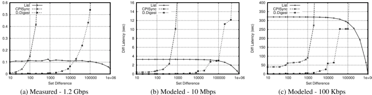
Key-Diff to compute the set of unique keys. Our results can be seen in Figure 11a. We note that there are 3 components contributing to the latency for all of these methods, the time to generate the response at hostB, the time to transmit the response, and the time to compare the response to the set stored at hostA. Since we maintain each data structure online, the time for hostBto generate a response is negligible and does not affect the overall latency.

We see from these results that theListshows predictable per-formance across difference sizes, but performs particularly well rel-ative to other methods as the size of the difference increases beyond 20K. Since the size of the data sentdecreasesas the size of the dif-ference increases, the transmission time and the time to sort and compare atAdecrease accordingly. On the other hand, the Differ-ence Digest performs best at small set differDiffer-ences. Since the es-timator is maintained online, the estimation phase concludes very quickly, often taking less than 1 millisecond. We note that precom-puting IBF’s at various sizes is essential and significantly reduces the latency by the IBF’s construction at hostB at runtime. Fi-nally, we see that even though its communication overhead is very low, the cubic decoding complexity forCPISyncdramatically in-creases its latency at differences larger than 100.

In considering the resources required for each algorithm,List

requires4|SB|bytes in transmission and touches|SA|+|SB|

val-ues in memory. Difference Digest has a constant estimation phase of 15.3KB followed by an average of24dbytes in transmission and3d×hash_{_}count_{memory operations (3 fields in each IBF}

cell). Finally,CPISyncrequires only10dbytes of transmission to send a vector of sums from it’s linear equations, butd3_memory

operations to solve its matrix.

If our experimental setup were completely compute bound, we would expectListto have superior performance for large differ-ences and Difference Digest to shine for small difference. If we assume ahash_countof 4, then Difference Digest’s latency is

12d, whileList’s is|SA|+|SB|= 2|SA| −d. Thus, they will

have equivalent latency atd= 2

12+1|SA|, or a difference of 15%.

Guidance for Constrained Computation. We conclude that, for our high-speed test environment, precomputed Difference Di-gests are superior for small deltas (less than 2%), while sending a full list is preferable at larger difference sizes. We argue that in environments where computation is severely constrained relative to bandwidth, this crossover point can reach up to 15%. In such scenarios, precomputation is vital to optimizediffperformance.

Varying Bandwidth. We now investigate how the latency of each algorithm changes as the speed of the network decreases. For this we consider bandwidths of 10 Mbps and 100Kbps, which are speeds typical in wide-area networks and mobile devices, respec-tively. By scaling the transmission times from our previous exper-iments, we are able to predict the performance at slower network speeds. We show these results in Figure 11b and Figure 11c.

As discussed previously, the data required byList,CPISync, and Difference Digests is4|SB|,10dand roughly24d, respectively.

Thus, as the network slows and dominates the running time, we ex-pect that the low bandwidth overhead ofCPISyncand Difference Digests will make them attractive for a wider range of deltas ver-sus the sortedList. With only communication overhead,List

will take4|SB|= 4(|SA| −d), which will equal Difference

Di-gest’s running time atd= 4

24+4|SA|, or a difference of 14%. As

the communication overhead for Difference Digest grows due to widely spaced precomputed IBF’s the trade off point will move to-ward differences that are a smaller percentage of the total set size. However, for small to moderate set sizes and highly constrained bandwidths KeyDiff should create appropriately sized IBF’s on de-mand to reduce memory overhead and minimize transmission time.

Guidance for Constrained Bandwidth.As bandwidth becomes a predominant factor in reconciling a set difference, the algorithm with the lowest data overhead should be employed. Thus, List

will have superior performance for differences greater than 14%. For smaller difference sizes, IBF will achieve faster performance, but the crossover point will depend on the size increase between precomputed IBF’s. For constrained networks and moderate set sizes, IBF’s could be computed on-demand to optimize communi-cation overhead and minimize overall latency.

7. CONCLUSIONS

We have shown how Difference Digests can efficiently compute the set difference of data objects on different hosts using computa-tion and communicacomputa-tion proporcomputa-tional to the size of the set differ-ence. The constant factors are roughly 12 for computation (4 hash functions, resulting in 3 updates each) and 24 for communication (12 bytes/cell scaled by two for accurate estimation and decoding). The two main new ideas are whole set differencing for IBF’s, and a new estimator that accurately estimates small set differences via a hierarchy of sampled IBF’s. One can think of IBF’s as a particularly simple random code that can deal with both erasures and insertions and hence uses a simpler structure than Tornado codes but a similar decoding procedure.

We learned via experiments that 3 to 4 hash functions work best, and that a simple rule of thumb is to size the second phase IBF equal to twice the estimate found in the first phase. We implemented Difference Digests in a KeyDiff service run on top of TCP that can be utilized by different applications such as Peer-to-Peer file transfer. There are three calls in the API (Figure 4): calls to add and delete a key, and a call to find the difference between a set of keys at another host.

In addition, using 80 cells per strata in the estimator worked well and, after the first 7 strata, augmenting the estimator with

(12)

0 0.1 0.2 0.3 0.4 0.5 0.6 10 100 1000 10000 100000 1e+06

Diff Latency (sec)

Set Difference List CPISync D.Digest (a) Measured - 1.2 Gbps 0 2 4 6 8 10 12 14 16 10 100 1000 10000 100000 1e+06

Diff Latency (sec)

Set Difference List CPISync D.Digest (b) Modeled - 10 Mbps 0 50 100 150 200 250 300 350 400 10 100 1000 10000 100000 1e+06

Diff Latency (sec)

Set Difference List

CPISync D.Digest

(c) Modeled - 100 Kbps

Figure 11: Time to run KeyDiffdifffor|SA|= 1M keys and varying difference sizes. We show our measured results in 11a, then

extrapolate the latencies for more constrained network conditions in 11b and 11c.

wise hashing provides better accuracy. Combined as a Difference Digest, the IBF and Hybrid Estimator provide the best performance for differences less than 15% of the set size. This threshold changes with the ratio of bandwidth to computation, but could be estimated by observing the throughput during the estimation phase to choose the optimal algorithm.

Our system level benchmarks show that Difference Digests must be precomputed or the latency for computation at runtime can swamp the gain in transmission time compared to simple schemes that send the entire list of keys. This is not surprising as computing a Dif-ference Digest touches aroundtwelve32-bit words for each key processed compared toone 32-bit word for a naive scheme that sends a list of keys. Thus, the naive scheme can be 10 times faster than Difference Digestsif we do no precomputation. However, with precomputation, if the set difference is small, then Difference Di-gest is ten times or more faster. Precomputation adds only a few microseconds to updating a key.

While we have implemented a generic Key Difference service using Difference Digests, we believe that a KeyDiff service could be used by some application involving either reconciliation or dedu-plication to improve overall user-perceived performance. We hope the simplicity and elegance of Difference Digests and their appli-cation to the classical problem of set difference will also inspire readers to more imaginative uses.

8. ACKNOWLEDGEMENTS

This research was supported by grants from the NSF (CSE-2589 & 0830403), the ONR (N00014-08-1-1015) and Cisco. We also thank our shepherd, Haifeng Yu, and our anonymous reviewers.

9. REFERENCES

[1] Data domain. http://www.datadomain.com/. [2] B. Bloom. Space/time trade-offs in hash coding with

allowable errors.Commun. ACM, 13:422–426, 1970. [3] A. Broder. On the resemblance and containment of

documents.Compression and Complexity of Sequences, ’97. [4] A. Z. Broder, M. Charikar, A. M. Frieze, and

M. Mitzenmacher. Min-wise independent permutations.J. Comput. Syst. Sci., 60:630–659, 2000.

[5] J. Byers, J. Considine, M. Mitzenmacher, and S. Rost. Informed content delivery across adaptive overlay networks. InSIGCOMM, 2002.

[6] J. W. Byers, M. Luby, M. Mitzenmacher, and A. Rege. A digital fountain approach to reliable distribution of bulk data. InSIGCOMM, 1998.

[7] G. Cormode and S. Muthukrishnan. What’s new: finding significant differences in network data streams.IEEE/ACM Trans. Netw., 13:1219–1232, 2005.

[8] G. Cormode, S. Muthukrishnan, and I. Rozenbaum. Summarizing and mining inverse distributions on data streams via dynamic inverse sampling.VLDB ’05. [9] D. Eppstein and M. Goodrich. Straggler Identification in

Round-Trip Data Streams via Newton’s Identities and Invertible Bloom Filters.IEEE Trans. on Knowledge and Data Engineering, 23:297–306, 2011.

[10] L. Fan, P. Cao, J. Almeida, and A. Broder. Summary cache: a scalable wide-area web cache sharing protocol.IEEE/ACM Transactions on Networking (TON), 8(3):281–293, 2000. [11] J. Feigenbaum, S. Kannan, M. J. Strauss, and

M. Viswanathan. An approximateL1_{-difference algorithm}

for massive data streams.SIAM Journal on Computing, 32(1):131–151, 2002.

[12] P. Flajolet and G. N. Martin. Probabilistic counting algorithms for data base applications.J. of Computer and System Sciences, 31(2):182 – 209, 1985.

[13] M. T. Goodrich and M. Mitzenmacher. Invertible Bloom Lookup Tables.ArXiv e-prints, 2011. 1101.2245. [14] P. Indyk and R. Motwani. Approximate nearest neighbors:

towards removing the curse of dimensionality.STOC, 1998. [15] M. Karpovsky, L. Levitin, and A. Trachtenberg. Data

verification and reconciliation with generalized error-control codes.IEEE Trans. Info. Theory, 49(7), july 2003.

[16] P. Kulkarni, F. Douglis, J. Lavoie, and J. M. Tracey. Redundancy elimination within large collections of files. In

USENIX ATC, 2004.

[17] Y. Minsky, A. Trachtenberg, and R. Zippel. Set reconciliation with nearly optimal communication complexity.IEEE Trans. Info. Theory, 49(9):2213 – 2218, 2003.

[18] R. Motwani and P. Raghavan.Randomized Algorithms. Cambridge Univ. Press, 1995.

[19] S. Muthukrishnan. Data streams: Algorithms and applications.Found. Trends Theor. Comput. Sci., 2005. [20] R. Schweller, Z. Li, Y. Chen, Y. Gao, A. Gupta, Y. Zhang,

P. A. Dinda, M.-Y. Kao, and G. Memik. Reversible sketches: enabling monitoring and analysis over high-speed data streams.IEEE/ACM Trans. Netw., 15:1059–1072, 2007. [21] B. Zhu, K. Li, and H. Patterson. Avoiding the disk bottleneck