Screen - Work package 4*

(1)

Screen - Work package 4

*

Assessing the Sectoral Effects

of ICT Investments

The Case of Broadband Networks

*Elton Beqiraj, Flavio Gazzani, Massimiliano Tancioni

under the coordination of Maurizio Franzini

Sapienza University of Rome - Department of Economics and Law

(2)

SCREEN- WORK PACKAGE4

2

List of abbreviations

ARDL Autoregressive Distributed Lags Process BN Broadband Networks

CPA Classification of Products by Activity ECM Error Correction Model

ESA European System of Accounts

ICT Information and Communication Technology

I/O Input Output

ITU International Telecommunication Union

IO-DGEM Input/Output-based Dynamic General Equilibrium model ISIC International Standard Industrial Classification

Mbps Megabits Per Second

NACE Nomenclature Statistique des Activités Èconomiques STAN Structural Analysis

(3)

Preface

Italy's broadband network strategy has a relatively ambitious goal: to reach at least 85% of the population with a 100 Mbps connectivity within 2020, and for the remaining 15%, to ensure a download speed of at least 30 Mbps.

The Italian ICT network infrastructures currently ensure access to fast connections (>30 Mbps) to only 21% of buildings (European Commission, 2014), the worst performance among EU countries. The EU average points to a degree of penetration of 62%. In terms of population, Italy ensures very fast connections to less than 1%, against an EU average of 6%.

The technological gap to be filled is thus massive, and the private investment plans are not consistent with the goal of reducing, if not filling, this gap.

Based on these premises, the actions needed to fulfil the declared objectives of the Italian Government's broadband network strategy are supported by an amount of public resources close to 6 billion Euro, of which two are financed by European regional funds, and the remaining by European development funds, to be anticipated by the European Bank of Investments.

This analysis provides a quantitative evaluation of the expected medium term macroeconomic effects of these infrastructural investments. The study uses a structural macroeconomic model specifically designed to perform simulation analyses at a high degree of detail for the key macroeconomic and labour market variables.

To highlight the sensitivity of results to the size of the investment plan, we repeat the analysis considering three alternative scenarios. In the first, we assume an investment in broadband networks of 5 billion euro within 2020, i.e. an amount relatively close to the Italian government's agenda. In the second and third scenarios we repeat the analysis by assuming an investment equivalent to 8 and 12 billions euro, respectively. In the absence of relevant information about the exact timing of the invesment expenditures, we assume that the total amount of expenditure is uniformally distributed within the period 2016-2020.

In the following sections, a sketch of the background literature, of the methodology and of the main results of the analysis are provided. A more technical description of the model and more detailed results are reported in a dedicated appendix, provided separately to this research report.

(4)

SCREEN- WORK PACKAGE4

1 - Comparative studies on sectoral effects of ICT

investments

A growing body of literature has found a positive relationship between broadband penetration (including mobile broadband) and economic development. Results show an economically significant and robust effect of broadband diffusion on economic growth even in the time span of just over a decade. The review of research indicates that there are several methods to estimate the economic impact of broadband investments, including econometric techniques, input-output analysis and qualitative case studies. Variations in estimates may be due to the differences in the definition of ‘broadband’, the statistical methodology used, datasets underpinning the analysis and model specifications/shortfalls. However, to date, very few studies addressed the sectoral effects of ICT investments. These empirical studies show that effects generally conform to our expectations, especially for the “real estate” and “financial intermediation” sectors, where a strong positive impact is also observed in other countries.

In particular, Crandall et al., 2007 provide estimates of the effects of broadband penetration on both output and employment, in the aggregate and by sector in the US, using state level data. They find that non-farm private employment and employment in several industries is positively associated with broadband use. More specifically, for every one percentage point increase in broadband penetration in a state, employment is projected to increase by 0.2 to 0.3 percent per year. For the entire U.S. private non-farm economy, this suggests an increase of about 300,000 jobs (2007), assuming the economy is not already at “full employment” (the national unemployment rate being as low as it can be with a low, stable rate of inflation).

Crandall et al., 2007 also estimated that broadband offers benefits across all industrial sectors, and contribution to growth vary by industry sector. Increasingly, individuals use broadband at home to connect to their business offices or even to telecommute. Such activities are more likely to be important in the service industries, such as finance, real estate, or miscellaneous business services. The effect of broadband is most significant in explaining employment growth in education, health care, and financial services, but it is also significant for the growth of manufacturing employment. The latter result is somewhat surprising, as is the lack of an effect on employment growth in real estate.

Fornefeld et al., 2008 in collaboration with the Management Consulting GmbH (MICUS) on behalf of the European Commission, collected evidence of the economic impact of broadband internet on labour productivity, employment level and growth in the UK. The investigation focuses on the improvement of business processes through the use of online technologies in large companies. In the Cornwall Region, UK, Fornefeld et al., 2008 highlight that the strongest growth occurred in “real estate, renting and business activities” (NACE “Statistical Classification of Economic Activities in the European Community” section K) and “retail, wholesale and repair” (NACE section G). It reflects the fact that the service industry in Cornwall is of greater importance than the manufacturing industry. Real estate, renting and business activities is of specific relevance when trying to isolate the impact of broadband on the economy: it includes all “computer and related activities” and thus companies offering business services who are major

(5)

ASSESSING THESECTORALEFFECTS OFICTINVESTMENTS- THECASE OFBROADBANDNETWORKS

beneficiaries of broadband usage. Productivity in Cornwall is low (which is reflected in its lower wage level). This is partly due to the economic structure of Cornwall, with high shares of activity in economic sectors with low productivity. In contrast, in the business services sector, productivity rose considerably after broadband became available in Cornwall. Yearly growth in productivity more than quadrupled and reached 11.5% between 2001 and 2005. During the same time period, productivity only increased by 4% across the UK in the business services sector.

In Australia, the Centre for International Economics (CEI, 2014) conducted a study on the economic impacts of broadband on the Australian economy using a computable general equilibrium model to translate direct changes into overall impacts on the size and structure of the Australian economy. This model (53-sector and 8 region) found out that the largest impacts in 2013 occur in sectors that produce capital, such as construction sectors and in real estate sector. This is because the change in household income leads to a higher demand for dwelling services - satisfying this demand requires a significant increase in construction activity in the short term. This increase in construction activity will be largely temporary. Construction sectors also cited a relatively large productivity impact from their use of mobile broadband. The sectors least impacted are agricultural production and oil and gas production, where the impacts on output are less than 1 per cent.

Katz et al., 2010 quantifies the macroeconomic impact of investment in broadband technology on employment and output of Germany’s economy. Two sequential investment scenarios were analyzed: the first by the German Government which aims at ensuring that 75 percent of German households have access to a broadband connection of at least 50Mbps by 2014. The second scenario (labeled "ultrabroadband" covering 2015-2020) defines the investment required to provide to 50 percent of households with at least 100 Mbps and another 30 percent with 50 Mbps by 2020. The economic model was based on input-output tables from the German Federal Statistical Office. The study indicates that the labour intensive nature of broadband deployment implies significant effect on the construction sector and, despite the high technological nature of the ultimate product, broadband is to be seen as economically meaningful as conventional infrastructure investments, such as roads and bridges.

Against these findings from overseas evidence related to broadband and mobile technology investments, Italian evidence for ICT suggests similar impacts in real estate renting and business activities and financial intermediation sector and lower impacts on mining and quarrying, manufacturing and agriculture sector. A larger amount of the growth impact is from productivity gains rather than capital deepening, which again is consistent with the relatively inexpensive nature of mobile broadband compared to the significant costs of ICT investment and this condition vary consistently in each country.

(6)

1 - Methodology

2.1 - Simulation

The analysis is conducted through the simulation of an Input/Output-based Dynamic General Equilibrium model (IO-DGEM) of the Italian economy, conditional to an expected exogenous variation in investment in broadband internet networks (BNs). The sections below provide the details of the simulation strategy, by detailing, at a non technical level, the IO-DGEM's basic features and the ingredients considered in the definition of the the investment scenarios1_.

2.1.1 - The model: main features

In this section we provide the basic elements of the methodology adopted for the construction of an industry-level macro-economic model for the simulation of the economic effects of investments in BNs. From the point of view of the official statistical information, BNs are included in the Telecommunication sector accounts and in its disaggregation into the Internet, Mobile telephony and Fixed telephony sub-sectors.

The research objective is to evaluate the impact of ICTs investments on the produced output and on employment in the other sectors in the economy. This requires an evaluation of how the Telecommunications sector and in particular the Internet, Mobile telephony and Fixed telephony sub-sectors affect the productive capabilities of other sub-sectors as intermediate input through the identification of the direct supply effects and indirect price and demand effects.

The consideration of the latter (indirect price composition and demand effects) is essential to the analysis and distinguishes the proposed approach from more standard analyses, mainly based on the design and simulation of the sole supply side of the economy.

The analysis relies on an estimated/calibrated general equilibrium model, whose supply-side is based on input-output relationships among industries, and the demand side is fully specified under the hypothesis of monopolistic competition, such that firms are price-setters, i.e. they consider a mark-up over marginal costs in their pricing decisions, and demand is defined considering the full set of industry-specific relative prices.

Production takes place considering an input/output production technology in which the input mix is chosen optimally based on the relative prices of intermediate factor inputs. The telecommunication sector is isolated, detailed into its mobile, fixed telephony and internet subsectors, and included into the several production functions, such that a simulated investment decision affects each sector both directly and indirectly through the other sectors' responses. The impact in each sector is captured by an increase in the telecommunication input, leading to production effects and substitution effects, the latter driven by relative price changes.

___________________________

1_{A more technical discussion of the model structure is provided in a dedicated document to this study report.}

SCREEN- WORK PACKAGE4

6

(7)

A flexible translog production technology employing 16 factor inputs is adopted for describing the supply side: sectors are those of the two-digits NACE classification (Rev. 1.1)2_{. The attractive feature of the} translog functional form is that it imposes no a priorirestrictions on substitution and price elasticities, that can be derived from the estimated parameters of the implied cost share functions. On the demand side, following a standard approach, sector-specific demand and price setting functions are analytically derived under the hypothesis of monopolistic competition.

The IO-DGEM thus provides an instrument that allows a scientific evaluation of the potential macroeconomic effects of BN investment decisions at a high level of detail. For expositional convenience, the simulation results will be summarized considering only output variations, labour input variations and price changes3_.

Given the limited sample size and the nonlinearity of the key output production functions and of the related cost shares, the Bayesian estimator is employed to parameterize the supply side of the model. The parameterization of the demand side is instead calibrated.

The instantaneous and cumulated effects on output and employment are evaluated in terms of both percentage deviations from control (i.e. a situation in which no investment occurs) and in terms of variations of volumes, i.e. output value effects (in Euro), and employment effects (in jobs).

The estimation requires detailed statistical information on sectoral outputs and inputs, i.e. industry by industry input-output tables, publicly provided by the Eurostat (European System of Accounts - ESA 95), while information on other operational variables and data are obtained from the Eurostat Structural Indicators and from the STAN - OECD database. A detailed description of the statistical information is provided in the next section.

2.1.2 - Data sources

The model parameterization is obtained from the information provided by a panel of years and sectors. The time-period ranges from 1995 to 2014. According to the 2-digit NACE classification systems, 58 production sectors are included in the estimates and in the model simulation (NACE-P is omitted because of data constraints). These 58 economic sectors cover all the economic activities, that is, only mentioning the macro-areas (1-digit NACE): Agriculture, hunting and forestry (A), Fishing (B), Mining and quarrying (C), Manufacturing (D), Electricity, gas and water supply (E), Construction (F), Wholesale and retail trade, repair of motor vehicles, motorcycles and personal and household goods (G), Hotels and restaurants (H), Transport, storage and communication (I), Financial intermediation (J), Real estate, renting and business activities (K), Public administration and defense; compulsory social security (L), Education (M), Health and social work (N), Other community, social and personal service activities (O).

___________________________

2 _{NACE is a 4-digit activity classification used by the European Union since 2002. More details are available at:}

http://ec.europa.eu/eurostat/ramon/relations/index.cfm. The classification of economic activities according to NACE is totally coherent with ISIC and can be considered its European counterpart. Concordance tables from NACE to ISIC are available at: http://www.foost.org/database/nace/nace-en_2002c.php.

3_{The full model output can be obtained upon request.}

(8)

The econometric analysis relies on the following set of data:

- values of the 1-digit 17 inputs used (included labour) at purchaser prices - values of the 2-digit sectoral output at basic prices

- inputs’ prices (except labour) - labour compensation

All this information is obtained by three main data sources: (1) OECD – STAN STructural ANalysis Database;

(2) Eurostat - Industry, trade and services – Industry and construction Industry; (3) ESA 95 Table – Input-output tables – Eurostat.

In details:

- Inputs and Outputs at basic prices are obtained from all the sectors (A/01-Q/99) ESA 95 Table - Input-output tables - Eurostat: Supply and Use Tables, Current Prices. Two-digit NACE aggregation system.

This dataset is key in definition of the model structure, i.e. of the number of production sectors, relative prices and demand functions being considered in the model, as well as for the model estimation stage. The supply, the use and the merged input-output tables provide a detailed picture of the interdependencies of the production system. In particular, information on the use of goods and services (products) and the output generated in each production is provided by the supply and use tables.

The symmetric input-output table is a transformation of the supply and use tables under a fully consistent classification system4_.

The supply table illustrates where in the production system goods and services are produced; in other words, it offers information on the supply of goods and services by type of product of an economy in each year. By column, information on the the production programme for each sector is provided, i.e. the domestic output of primary and secondary productions is reported. The main activities of each industry are identifiable along the main diagonal of the matrix table, whereas the off-diagonal elements provide information on secondary activities.

The use table conveys information on the use of goods and services by product, by type of use for intermediate consumption (i.e. where intermediate consumption by industry is paired to final consumption by individuals) and by industry. Its structure can be described as follows: by columns, the input structure of each industry is reported; by row, instead, the use of different products and primary inputs is shown for each production sector. The costs of production can be obtained in the table's columns for each sector and the total cost of each product can be obtained from the sum across columns for each row. The total output measured at basic prices for each sector is reported as sum across rows for each column.

The use input-output table is the results of intersections between (rows) product and value added and (columns) sectors and individuals as final users (exemplified in Table 2.1). The rows report the use of SCREEN- WORK PACKAGE4

8

___________________________

4 _{The classification used for the included sectors is the "General Industrial Classification of Economic Activities within the} European Communities" (NACE), whereas the classification employed for products is the ‘Classification of Products by Activity’ (CPA), which are one the counterpart of the other.

(9)

goods and services by sector (intermediate consumption) and by individuals (final consumption). The columns of sectors reflect the production structure (used inputs) of each specific sector.

Table 2.1 - Structure of a use I/O table of an economic system composed by only 3 sectors (Agriculture, Manufacture and Transport).

In the example reported in Table 2.2 below, 10% of the cereal production is used as input in the productive process of agriculture and 33% in manufacture. 57% is consumed by individuals. With respect to columns, the transport sector employs 50% of textiles and 50% of transport services for the total production of 15 units.

Table 2.2 - Example of a use I/O table of an economic system composed by only 3 sectors (Agriculture, Manufacture and Transport).

The combination of the supply and the use tables gives the symmetric input-output table, which requires a transformation procedure in order to pass from the product by industry system of the supply and use tables to the product by product system or the industry by industry system.

It is worth stressing that, given the single output technology hypothesis, which implies that a sector produces a single product/service, the only needed information for the purposes of our analysis is the use input-output tables (made by 58 rows and 17 columns).

ASSESSING THESECTORALEFFECTS OFICTINVESTMENTS- THECASE OFBROADBANDNETWORKS

9

Products _{Agriculture Manufacture Transport}Sectors Final users TOTAL

Cereals Textiles

Transport services

Intermediate consumption Final consumption

by product

Total consumption

by product

Value added Value added by sector Total Value added

TOTAL Total output by sector Total consumption

by final users

Products _{Agriculture Manufacture Transport}Sectors Final users TOTAL

Cereals Textiles Transport services 57 41 19 110 118 68 Value added 12 TOTAL 117 10 33 0 5 67 5 21 23 5 2 5 5 38 128 15

(10)

Price deflators for the industries/productions of the Supply and Use Tables are obtained from different sources' data elaborations and harmonization. Data from STAN are sometimes aggregated at a less detailed ISIC level. In this case, average prices as given by STAN in the ISIC category are used. For instance, agriculture and fishing that are in the ISIC group 01_02 are distinct categories in NACE. To this purpose, the same price (given by STAN) within the ISIC_group 01_02 was associated to the two categories 01 and 02 in the NACE classification. The associated price is the average of the prices in sectors agriculture and fishing weighted by the relative output shares. In the specific of the various sectors, the following data sources are considered:

• Agriculture, hunting and forestry (A/01-02): OECD - STAN - Two-digit ISIC aggregation system • Fishing (B/05): OECD - STAN - Two-digit ISIC aggregation system

• Mining and quarrying (C/10-14): OECD - STAN - Two-digit ISIC aggregation system

• Manufacturing (D/1537): Eurostat Industry, trade and services Industry and construction -Industry - Production price indices - Two-digit NACE Rev. 1 aggregation system

• Electricity, gas and water (E/40-41): OECD - STAN - Two-digit ISIC aggregation system • Construction (F/45): OECD - STAN - Two-digit ISIC aggregation system

• Wholesale and retail trade; repair of motor vehicles, motorcycles and personal and house-hold goods (G/50-52): OECD - STAN - Two-digit ISIC aggregation system

• Hotels and restaurants (H/55): OECD - STAN - Two-digit ISIC aggregation system

• Transport, storage and communication (I/60-64): OECD - STAN - Two-digit ISIC aggregation system • Financial intermediation (J/65-67): OECD - STAN - Two-digit ISIC aggregation system

• Real estate, renting and business activities (K/70-74): OECD - STAN - Two-digit ISIC aggregation system

• Public administration and defence; compulsory social security (L/75): OECD - STAN - Two-digit ISIC aggregation system

• Education (M/80): OECD - STAN - Two-digit ISIC aggregation system

• Health and social work (N/85): OECD - STAN - Two-digit ISIC aggregation system

• Other community, social and personal service activities (O/90-93): OECD - STAN - Two-digit ISIC aggregation system

• Activities of households (P/95): OECD - STAN - Two-digit ISIC aggregation system

• Extra-territory organizations and bodies (Q/99): OECD – STAN - Two-digit ISIC aggregation system

Employment is obtained as a result of some elaborations. Data from all sectors (A/01Q/99) STAN -Two-digit ISIC aggregation system - Total employment (number of persons employed) are sometimes aggregated at a less detailed ISIC level than in the I/O tables. In these cases, STAN provides the aggregate value for employment, i.e. total workers in the ISIC category are used, and these aggregates are spread into the relevant subcategories by using a schedule of weights based on relative output shares obtained from the NACE sub-categories.

- Labour compensation, i.e. the wage rates (basic wages, cost-of-living allowances, and other guaranteed and regularly paid allowances) + ii) overtime payments + iii) bonuses and gratuities regularly paid + iv) remuneration for time not worked + v) bonuses and gratuities irregularly paid + vi) payments SCREEN- WORK PACKAGE4

10

(11)

in kind + vii) employer contribution to statutory social security schemes or to private funded social insurance schemes + viii) unfunded employee social benefits paid by employers, are obtained from the all sectors (A/01-Q/99) OECD - STAN - Labour compensation - Two-digit ISIC aggregation system.

2.1.3 - Model output

The effects of BN investments is tracked by the impulse response functions of the following key variables:

• Percentage output deviation from control. This measure defines the percentage variation in output due to the BN investment with respect to a situation in which the shock does not occur (i.e. at the equilibrium). The percentage output deviation in the case of BN investments is, for all economic sectors, positive or at most zero. The effects can be evaluated as simple deviations from control or in terms of cumulated changes. Since the I/O-DGEM is scaled with respect to the total value of production, sector-specific output variations (instantaneous or cumulated) can also be reported in terms of values (millions of euro).

• Percentage employment deviation from control. This measure defines the percentage variation in labour input demand due to BN investments, evaluated with respect to a situation in which the shock does not occur (i.e at the equilibrium). The percentage employment deviation is positive for some economic sectors and negative for the others. More labour is used in sectors in which the variation in relative prices leads to a variation in demand which is higher than that in the production potential. Other sectors will experience an employment contraction, taking place because of high input factors substitution elasticity and/or a dampened response of demand with respect to the production potential response. It is impossible to define, within a general change in the labour measure, the relative effects on hours worked, employment and effort. In the real world, these depend on a large number of aspects such as the severity of the investment shock, the time length of its physical implementation, its time profile and the labour market conditions. Similar to the output change, the employment effects can be evaluated as simple deviations from control or in terms of cumulated changes. Furthermore, from the sector-specific equilibrium employment data and the employment impulse responses, it is possible to recover the sector specific employment variations in terms of number of job gains/losses.

• Percentage price deviation from control. This measure defines the variation of single products (thus relative) prices which necessary to restore the equilibrium condition after a BN investment shock. Price variations are not the real-world ones but express the variation of the sectoral price indexes (year 2010 = 100) which is consistent with the satisfaction of the equilibrium conditions. The price variation is expected to be generally negative or unsignificant for all economic sectors, because the increase in the output potential in a specific sector directly causes the decrease of its output price. However, second round effects from the demand side can cause sign reversion in sectors in which a high demand elasticity to relative prices leads to more than proportional increases in demand with respect to the increases in potential output.

(12)

2.1.4 - Some caution on the reliability of results

It is worth stressing that, because of the stylized nature of the model, results necessarily provide only an approximate evaluation of the potential macroeconomic and sectoral effects from the implementation of the BN investment plans.

A first element of caution is that, in the current model version, the labour market is specified under the hypothesis of perfect competition and flexible wages (i.e. a Walrasian labour market), such that the employment response tends to be under-estimated, because of the high degree of wage flexibility, dampening the response of the labour input. The hypothesis of price flexibility also plays a role in model dynamics, ensuring that a relevant fraction of the real variability introduced by the shocks is absorbed by the price dynamics. Moreover, because of the monetary neutrality resulting from the peculiar theoretical assumptions behind the specific model design, the inflation/deflation dynamics are not expected to open-up a monetary transmission channel of the shock, i.e. through variations in the expected real interest rate. The latter limitation is of particular relevance in the present economic environment, characterized by the presence of a persistent liquidity trap in which the nominal interest rate is stuck at the zero lower bound. In such circumstances, a deflationary shock (as it is, in principle, the BN investment shock) might trigger an increase of the real interest rate, inducing a short term aggregate demand and employment contraction. The presumed expansionary effects of the policy can thus be jeopardized.

These model drawbacks, that are typical of flexible price DGE models, can be removed by designing the relevant nominal and real rigidities characterizing the functioning of real economies. These modifications are currently being implemented, thus their relevance for results can be appreciated in future applications of the model. Note however that these under-specification biases are more important for the short term model dynamics, whereas the medium and long term results should be only marginally affected, since the effects of nominal/real rigidities tend to vanish over time.

2.1.5 - The simulation scenario: from public investments to ICT output changes

Aggregated effects of BN investments are evaluated by shocking the production technology of the Telecommunications sector (I61.1 in the three-digit NACE classification)5_{. Technically, the impulse} responses of output, prices, wages and labour input are conditional to a shift factor affecting the Telecommunications production function.

The ICT production shift factor, expressed in value of sector specific output (BB_V), is obtained econometrically, by estimating the sensitivity of the ICT production capability to a change in the BN infrastructures (BB_L), in turn estimated as a function of the BN investment (INV_BN).

The production shifter is thus defined in three conceptual steps: the starting point of the analysis is the deterministic (thus expected) simulation of the BN investment shock, calibrated to be equivalent to a fraction of output equal to 5, 8 and 12 billion of Euros within 2020, defining the first (S1), second (S2) and third (S3) investment expenditures scenario. In the second step, an estimated relation between BN SCREEN- WORK PACKAGE4

12

___________________________

5 _{Due to the fact that input-output tables and, as consequences, sectoral interdependencies are provided by Eurostat at} maximum detail at two-digit level, the Telecommunications sector has been isolated by the Post and Telecommunications sector according to its weight in the sector I61 of the two-digit classification. The relative weight of the Telecommunication sector in Post and Telecommunications is nearly 70% for Italy.

(13)

infrastructures (broadband lines) and BN investment (value) is employed to obtain the variation induced by the change in BN investment to the BN network physical infrastructure, in order to evaluate the change in the physical production potential. In the third step, an estimated relation between the value of the ICT production and the physical BN infrastructure is employed to obtain the change in the ICT production potential in value (i.e. the shift factor of interest, BB_V).

Three equations characterize the above mentioned steps: i) a first order autoregressive process (AR1) or as explicit hypothesis denote the time the investment shock INV_BN; ii) an autoregressive distributed lags process (ARDL) for the relation between physical infrastructures BB_L and BN investment; iii) an autoregressive distributed lags process (ARDL) for the relation between the value of the ICT production and physical infrastructures.

Formally:

where lower case letters indicate logs of level variables, ρis the memory coefficient for the investment process, and ε_tinv, ε_tbb_land ε_tbb_vare i.i.d. shocks.

Note that the ARDL(p,q) processes can have a long-run equilibrium representation (i.e. they can be co-integrating vectors), as well as a dynamic representation in terms of Dynamic Error Correction Model (ECM), which is the relevant representation in cases of non-stationarity and co-integration. We have verified that this is our case.

The three equations above thus provide the size and the shape of the investment stimulus to the I/O production structure of the model. Figures 1, 2 and 3 in the follwing pages show the dynamic patterns (deviations from control) for the three variablesinv_bnt, bb_ltand bb_vtin the three scenarios.

ASSESSING THESECTORALEFFECTS OFICTINVESTMENTS- THECASE OFBROADBANDNETWORKS

13

The production shifter is thus defined in three conceptual steps: the starting point of the analysis is the stochastic simulation of the BN investment shock, calibrated to be equivalent to a fraction of output equal to 6 billion of Euros within 2020, coherently with the Italian government's agenda. In the second step, an estimated relation between BN infrastructures (broadband lines) and BN investment (value) is employed to obtain the variation induced by the change in BN investment to the BN network physical infrastructure, in order to evaluate the change in the physical production potential. In the third step, an estimated relation between the value of the ICT production and the physical BN infrastructure is employed to obtain the change in the ICT production potential in value (i.e. the shift factor of interest, BB_V).

Three equations characterize the above mentioned steps: i) a first order autoregressive process (AR1) for the investment shock INV_BN; ii) an autoregressive distributed lags process (ARDL) for the relation between physical infrastructures BB_L and BN investment; iii) an autoregressive distributed lags process (ARDL) for the relation between the value of the ICT production and physical infrastructures. Formally: !"#!!"! !!!"#!!"!!1!!tinv !!!!!! !!!"! !! ! !!1 !!!!!!!! !! ! !!0 !"#!!"!!!!!t bb!l !!!!! !!!!"! !! ! !!1 !!!!!!!! !! ! !!0 !!!!!!!!!t bb!v

where lower case letters indicate logs of level variables, !is the memory coefficient for the investment process, and !tinv!!tbb!l and !tbb!v are i.i.d. shocks.

Note that the ARDL(p,q) processes can have a long-run equilibrium representation (i.e. they can be co-integrating vectors), as well as a dynamic representation in terms of Dynamic Error Correction Model (ECM), which is the relevant representation in cases of non-stationarity and co-integration. We have verified that this is our case.

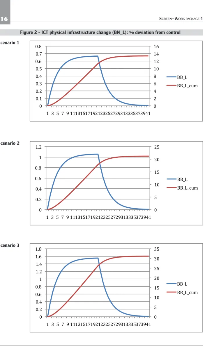
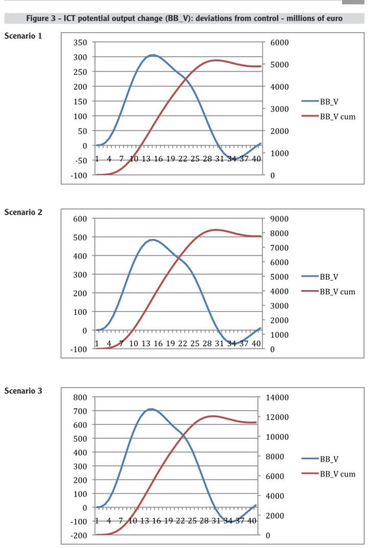
The three equations above thus provide the size and the shape of the investment stimulus to the I/O production structure of the model. Figures 1, 2 and 3 below show the dynamic patterns (deviations from control) for the three variables inv_bn, bb_l and bb_v.

Note that, under an ARDL modelling structure, the presence of co-integration emerges naturally from the long-run (steady state) solution of the dynamic equations. In our setting, the long-run forcing variable is the investment shock inv_bn, such that the second equation of the above three leads to the following long-run solution for bb_lt.

Note that, under an ARDL modelling structure, the presence of co-integration emerges naturally from the long-run (steady state) solution of the dynamic equations. In our setting, the long-run forcing variable is the investment shock inv_bn, such that the second equation of the above three leads to the following long-run solution for !!!_!.

!!!!!_! ! !! !_!_!1!! ! !" !! !_!_!1!! ! !! ! !!0 !"#!!"! !! !_!_!1!!

Because of the third of the three dynamic equations, the long-run (equilibrium) solution for the value of the broadband production !!!!reads as follows:

!!!!!_! ! !! !!!1!! ! !" !! !!!1!! ! !! ! !!0 !!!!! !! !!!1!!

The two steady-state relations show that the investment shock implies non-zero long-run effects in both broadband infrastructures and in the value of their production potential.

Given the positions above, the dynamic adjustments to the steady state solutions are driven by the simulation of the error-correction (ECM) transformation, i.e.:

!!!!!! !!! !! !!! !!1 !!!!!!!!! !! !!! !!0 !"#!!"!!!!!t bb_l !!!!!! !!! !! ! !!1 !!!!!!! ! !! ! !!0 !!!!!!!!!t bb!v

The ECMs thus provide the transitory deviations from the time-evolving long-run equilibrium of the level variables, whereas the simulation of the ARDL provides the dynamic effects of the investment shock in (the level of) broadband infrastructures and in the (level of) value of its production potential.

In other terms, the cumulated effects of the percentage deviation from control denote the expected effects of interest of our analysis.

(14)

SCREEN- WORK PACKAGE4

14

Because of the third of the three dynamic equations, the long-run (equilibrium) solution for the value of the broadband production bb

vtreads as follows:

Note that, under an ARDL modelling structure, the presence of co-integration emerges naturally from the long-run (steady state) solution of the dynamic equations. In our setting, the long-run forcing variable is the investment shock inv_bn, such that the second equation of the above three leads to the following long-run solution for !!!!.

!!!!!_! ! !! !!!1!! ! !" !! !!!1!! ! !! ! !!0 !"#!!"! !! !!!1!!

!!!!! _! ! !! !_!_!1!! ! !" !! !_!_!1!! ! !! ! !!0 !!!!! !! !_!_!1!!

!!!!!! !!! !! !!! !!1 !!!!!!!!! !! !!! !!0 !"#!!"!!!!!t bbl !!!!!! !!! !! ! !!1 !!!!!!!! !! ! !!0 !!!!!!!!!t bb!v

Note that, under an ARDL modelling structure, the presence of co-integration emerges naturally from the long-run (steady state) solution of the dynamic equations. In our setting, the long-run forcing variable is the investment shock inv_bn, such that the second equation of the above three leads to the following long-run solution for !!!_!.

!!!!!_! ! !! !_!_!₁!_!! !" !! !_!_!₁!_!! !! ! !!0 !"#!!"! !! !_!_!₁!_!

!!!!!_! ! !! !!!1!! ! !" !! !!!1!! ! !! ! !!0 !!!!! !! !!!1!!

!!!!!! !!! !! !!! !!1 !!!!!!!!! !! !!! !!0 !"#!!"!!!!!t bb_l !!!!!! !!! !! ! !!1 !!!!!!! ! !! ! !!0 !!!!!!!!!t bb!v

(15)

ASSESSING THESECTORALEFFECTS OFICTINVESTMENTS- THECASE OFBROADBANDNETWORKS

15

Figure 1 - BN investment shock: values - millions of euro - Scenario 1-3

!

"! #"""! $"""! %"""! &"""! '"""! ("""! "! '"! #""! #'"! $""! $'"! %""! #! &! )! #"!#%!#(!#*!$$!$'!$+!%#!%&!%)!&"! ,-./0-!12345! ,-./0-!467!

!

"! #"""! $"""! %"""! &"""! '"""! ("""! )"""! *"""! +"""! "! '"! #""! #'"! $""! $'"! %""! %'"! &""! &'"! #! &! )! #"!#%!#(!#+!$$!$'!$*!%#!%&!%)!&"! ,-./0-!12345! ,-./0-!467! Scenario 1 Scenario 2

!

"! #"""! $"""! %"""! &"""! '""""! '#"""! '$"""! "! '""! #""! (""! $""! )""! %""! *""! '! $! *! '"!'(!'%!'+!##!#)!#&!('!($!(*!$"! ,-./0-!12345! ,-./0-!467! Scenario 3

(16)

SCREEN- WORK PACKAGE4

16

Figure 2 - ICT physical infrastructure change (BN_L): % deviation from control

!

"! #! $! %! &! '"! '#! '$! '%! "! "('! "(#! "()! "($! "(*! "(%! "(+! "(&! '! )! *! +! ,!''!')!'*!'+!',!#'!#)!#*!#+!#,!)'!))!)*!)+!),!$'! --./! --./.012!

!

"! #! $"! $#! %"! %#! "! "&%! "&'! "&(! "&)! $! $&%! $! *! #! +! ,!$$!$*!$#!$+!$,!%$!%*!%#!%+!%,!*$!**!*#!*+!*,!'$! --./! --./.012! Scenario 1 Scenario 2

!

"! #! $"! $#! %"! %#! &"! &#! "! "'%! "'(! "')! "'*! $! $'%! $'(! $')! $'*! $! &! #! +! ,!$$!$&!$#!$+!$,!%$!%&!%#!%+!%,!&$!&&!&#!&+!&,!($! --./! --./.012! Scenario 3

(17)

ASSESSING THESECTORALEFFECTS OFICTINVESTMENTS- THECASE OFBROADBANDNETWORKS

17

Figure 3 - ICT potential output change (BB_V): deviations from control - millions of euro

!

"! #"""! $"""! %"""! &"""! '"""! ("""! )#""! )'"! "! '"! #""! #'"! $""! $'"! %""! %'"!

#! &! *! #"! #%! #(! #+! $$! $'! $,! %#! %&! %*! &"!

--./! --./!012!

!

"! #"""! $"""! %"""! &"""! '"""! ("""! )"""! *"""! +"""! ,#""! "! #""! $""! %""! &""! '""! (""!

#! &! )! #"! #%! #(! #+! $$! $'! $*! %#! %&! %)! &"!

--./! --./!012! Scenario 1 Scenario 2

!

"! #"""! $"""! %"""! &"""! '""""! '#"""! '$"""! (#""! ('""! "! '""! #""! )""! $""! *""! %""! +""! &""! '! $! +! '"!')!'%!',!##!#*!#&!)'!)$!)+!$"! --./! --./!012! Scenario 3

(18)

The shift factor BB_V affects the production capabilities of the ICT sector, that are specified by a variant of the estimated production function of the Post and Telecommunication services, for which information is available.

This has required the identification of reliable statistical information and the collection of a large amount of data on proxy variables and their manipulation. To obtain the factor shares of the three sub-sectors (Internet, Fixed telephony and Mobile telephony) of the Telecommunications aggregate in each production sector of the economy, information on revenues of each sub-sector has been used to obtain their weights in the Telecommunications sector and then shares to calibrate the simulations. Datafor the decomposition of Telecommunication sectors in the three sub-sectors and the economic nature of the input-output data come from data on Internet, Mobile telephony and Fixed telephony revenues provided by the International Telecommunication Union (ITU).

The final effects of a BN investment shock on sector prices and quantities depend on specific features of the theoretical model and in particular on the chosen parameterization. On the supply side, key parameters are those defining inputs, partial elasticities in production, and price elasticities; on the demand side, the elasticity of substitution among differentiated products in demand and mark-ups over marginal costs also play an important role. Sector-specific partial elasticities in production are estimated, while the other structural parameters are calibrated on the basis of previous results and, in the absence of reliable evidence, according to the conventional practice.

3 - Results

3.1 - The economic impact of BN investments

This section provides some details and partial results of the specific sub-objective of the research: the measurement of the direct and indirect economic effects of investments in in ICTs, and in particular in BN infrastructure investments.

As anticipated in the description of methodologies, results are summarized by focusing on three impact variables: instantaneous and cumulative output variation, percentage and in value; instantaneous and cumulative employment variation, percentage and in number of created/destroyed jobs; instantaneous and cumulative price variation.

SCREEN- WORK PACKAGE4

18

(19)

19

Before providing a summary of the simulation results at the one-digit sector level (two-digit results are provided separately), it is worth showing the aggregate results for output, i.e. the simulated variation of the productive capabilities of the entire economy under the three scenarios (S1, S2 and S3), and the respective expenditure multipliers. Figures 4 and 5 summarize these results for ten-year ahead simulations (2016-2025).

Figure 4 - Cumulative output variations in the three scenarios: millions euro, 2016Q1 - 2025Q4.

It is interesting to note that the output effects are not fully linear, i.e. they are increasingly stronger for higher amounts of BN investments (Figure 1). Such a nonlinearity can be quantified from the inspection of the dynamic output multiplier, i.e. the ratio between the output and the expenditure variation in the three scenarios. Compared to the first simulation scenario, the output multiplier icreases by nearly 10 and 25%, for S12 and S3, respectively.

Figure 5 - Output multipliers in the three scenarios: 2016Q1 - 2025Q4.

!

"! #""! $""! %""! &""! '"""! '#""! '$""! '%""! '&""! #"'%( '! #"'%( )! #"'*( '! #"'*( )! #"'&( '! #"'&( )! #"'+( '! #"'+( )! #"#"( '! #"#"( )! #"#'( '! #"#'( )! #"##( '! #"##( )! #"#)( '! #"#)( )! #"#$( '! #"#$( )! #"#,( '! #"#,( )! -./01.20!3'! -./01.20!3#! -./01.20!3)!

!

"! "#$%! "#$&! "#$'! "#$(! "#"! "#"%! "#"&! %$"') "! %$"') *! %$"+) "! %$"+) *! %$"() "! %$"() *! %$",) "! %$",) *! %$%$) "! %$%$) *! %$%") "! %$%") *! %$%%) "! %$%%) *! %$%*) "! %$%*) *! %$%&) "! %$%&) *! %$%-) "! %$%-) *! ./0123"! ./0123%! ./0123*!

(20)

SCREEN- WORK PACKAGE4

20

In the following sections we provide the results of the analysis at the one-digit sector detail, in the three investment scenarios (S1, S2 and S3, respectively).

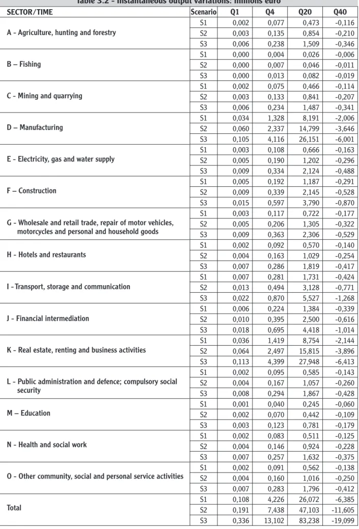
As highlighted in the preceding sections, for output and employment, results are given both in terms of volumes (millions of euro and job units) and in terms of percentage deviations from control. The volume measures provide an immediate indication of the expected sectoral effects of BN investments. However, since the economic relevance of each sector differs from that of other sectors, volumes do not provide a reliable measure of the relative impact of the measure, i.e. it is not a valid basis upon which comparing the sectoral effectiveness of the policy. In fact, an x% variation in a sector is different from the same x% variation in other sectors, with differences depending on the relative weight of each sector in the total economy. Comparative information is instead provided by the deviations from control results, i.e. the sectoral impulse response functions. For a more intuitive comparison, results are in this case summarized, for each variable and scenario, in radar graphs.

The sectoral value added effects of the broadband investment under the three scenarios are depicted in Table 3.2 (volumes, instantaneous effects), Figure 6 (percent deviations from control, cumulative effects) and Table 3.3 (volumes, cumulative effects). The information summarized therein shows that, at the aggregate level, by increasing the broadband investment from five to eight billion euro (i.e. 60% increase moving from S1 to S2), leads to an increase in the long-term (10 years) value added effects close to 74%. By increasing the investment to 12 billions euro (thus an increase from S2 to S3 equal to 50%), aggregate value added increases by an additional 75%. As shown by the implicit multiplier analysis, the effects on value added are thus increasing in the size of the broadband investment.

This result is mostly due to the nonlinearities in the relative price response and in the cost share functions, which are transferred into nonlinear production technology's re-compositions of the productive mix6_.

Figure 6 shows that the relative effects of the investment shock are higher in the Financial intermediation (J), Real estate, renting and business activities (K) and in the Transport, storage and Communication sectors.

These sectors are those for which the higher share of ICT input in the production technology is observed, and the highest degree of ICT input's partial elasticity is estimated. The investment in broadband is thus highly effective because it affects an important input factor in the sector-specific production potential, both in terms of the share in production and in the size of the degree of substitutability with other inputs. In fact, a high estimated partial elasticity of the ICT input implies that its use in production is strongly related to the changes in the relative price of factor inputs. Since the increase of supply of the broadband network leads to a drop in its unit price, a high partial elasticity implies that ICT use in these sectors increases even because of the switch to a more ICT-intensive production technology.

It is worth highlighting that the high sensitivity of the Real estate, renting and business activities is not surprising, since the Computer activities sector, observable only at the two-digits disaggregation level, belongs to this one-digit sector.

___________________________

6 _{We have verified that the behavior of the implicit multiplier with respect to the size of the investment stimulus is logistic,} i.e. it increases following an approximate exponential function for low levels of stimulus below 23 billion euro, above which saturation begins and the growth rate of the multiplier slows and asymptotically stops.

(21)

ASSESSING THESECTORALEFFECTS OFICTINVESTMENTS- THECASE OFBROADBANDNETWORKS

21

The relative effects of the broadband investment shock are instead minimal for the Education (M) and Health and social work (M) sectors. This result is justified by the fact that these sector's production potential of is only weakly related to the ICT input. Education and Health's production technologies, in fact, rely heavily on the labor input and on the non-ICT capital. Moreover, aside from the low share of ICT input in production, a small size of its partial elasticity to the relative price is estimated, indicating that the productivity improvements resulting from the composition effects in the production technology - in turn due to the drop in the ICT's relative price - are minimal.

The map of the effects changes when considering volumes. The highest increase in value added is observed for the Real estate, renting and business activities (K) and for the Manufacturing sectors (D).

Considering the absolute performance of the latter sector, this result is mostly due to its quite high share in aggregate value added. In fact, the ICT use in the manufacturing sector's production technology is close to the aggregate economy's average share, as it is for the partial elasticity to the relative price. The expected 10 years cumulated increase in Real estate, renting and business activities' value added under the three scenarios is of 146 (S1), 255 (S2) and 446 (S3) million euro. For the Manufacturing sector these values are 137 (S1), 238 (S2) and 418 (S3) million euro.

The lowest increase in the volume of value added is observed for the Education (M) and Fishing (B) sectors. Considering the former, this result is mostly due to the low ICT share in production, whereas it is due to the low share in aggregate value added in the case of the latter sector. The expected 10 years cumulated increase in the fishing sector's value added under the three scenarios is of 0.4 (S1), 0.7 (S2) and 1.3 (S3) million euro. For the Education sector these values are 4 (S1), 7 (S2) and 13 (S3) million euro.

The sectoral employment effects of the broadband investment shock under the three scenarios are depicted in Table 3.4 (jobs, instantaneous effects), Figure 7 (percent deviations from control, cumulative effects) and Table 3.5 (jobs, cumulative effects). Overall, the investment in broadband is expected to lead to a relatively moderate increase in employment. Considering the long-term effects (10 years), more than 56 thousands job positions are opened under scenario S1, whereas more than 98 thousands and 172 thousand jobs are created in the remaining scenarios (S1, and S2, respectively).

However, differently from the value added effects, the employment variation is strongly heterogeneous across sectors. Negative variations can in fact be observed both in the short and in the long term for some sectors. The sign of the employment variation calls into question the interplay between demand and supply effects. A negative employment response is observed in sectors where the output potential, thus productivity, increases more than the demand for its production. The response of the latter depends on the estimated elasticity of demand to the relative consumer price variation, as well as on the variation in aggregate demand. A positive employment response is instead observed when the single product's demand increases more than the sector-specific productivity.

Figure 7 shows that the relative employment effects of the investment shock are positive and higher in the Health and social work sector (N), Education (M) and in the Other community, social and personal service activities sector (O). A relatively high relative employment effect is also observed in the Hotels and restaurants (H), Manufacturing (D) and Fishing (B) sectors. The economic reason for these positive employment effects is that, as shown above, these sectors experience the lowest increase in the production potential from the broadband investment, because of the low ICT share in production and its weak partial

(22)

SCREEN- WORK PACKAGE4

22

elasticity to relative prices. Contemporaneously, the general increase in demand resulting from the price deflation leads to an increase in the sector-specific demand which is higher than the increase in productivity.

Because of this mechanism, the Real estate, renting and business activities sector (K), the Transport, storage and communication sector (I) and the Mining and quarrying sector (C) experience quite strong long-term employment contractions. For these sectors, the long-term increase in demand is not able to match the long-term increase in productivity.

Considering job variations, the highest increase in employment is observed for the Hotels and restaurants (H) and in the Manufacturing sectors (D). Similarly to the value added volume pictures, the employment performance of the latter sector is mostly due to its quite high share in aggregate employment. In fact, the increase in productivity and the increase in demand in this sector are close to aggregate economy's average results. The expected 10 years cumulated increase in Hotels and restaurants employment under the three scenarios is of 64 (S1), 111 (S2) and 195 (S3) thousands job positions. For the Manufacturing sector these values are 55 (S1), 96 (S2) and 168 (S3) thousands job positions.

The highest long-term decrease in employment is observed for the Real estate, renting and business activities sector (K), the Public administration and defense; compulsory social security sector (L).

The sectoral price effects of the broadband investment under the three scenarios are summarized in Table 3.6, reporting the instantaneous percent deviations from control, Figure 8, depicting the cumulative percent deviations from control, and in Table 3.7, reporting the cumulative percent deviations from control.

Overall, as Table 3.6 shows, the broadband investment under the three scenarios leads to a price reduction in all sectors, although the reduction tends to be quite heterogeneous in size across different sectors. It is worth noting that, on impact, the broadband investment shock does not affect the sector prices for almost all sectors, independently of the scenarios taken into consideration. This is due to the time-to-build and time-to-be-materialized effects of such policies.

In fact, considering the medium-term effects (one year) of the broadband investment shock under the three scenarios, a negative price variation characterizes all the sectors under analysis. The price reduction is characterized by a relatively strong heterogeneity among sectors. More precisely, a quite strong price reduction is observed in the Real estate, renting and business activities (K) and, although dampened, in the Transport, storage and communication sector (I), Financial intermediation (J), and Public administration and deference; compulsory social security (L).

As Table 3.6 reports, an overall and relatively high price reduction is also confirmed in the long-term (10 years). The sectors more affected by the investment shock are, in analogy with the medium term, the Real estate, renting and business activities (K) and, although dampened, the Transport, storage and communication sector (I), Financial intermediation (J), and Public administration and deference; compulsory social security (L).

The economic reason for these negative price variation is that, as shown above, these sectors are those benefiting most from the broadband investment shock, which leads to a significant and positive drop in marginal costs. Given the flexible price environment characterizing this sectors, the marginal cost reduction in production is translated into significant price reductions.

(23)

ASSESSING THESECTORALEFFECTS OFICTINVESTMENTS- THECASE OFBROADBANDNETWORKS

23

The lowest price reduction is instead observed in Health and social work (N), Education (M), and Other community, social and personal services activities (O) sectors.

Figure 8 depicts the cumulative effect of the broadband investment on price variation under the three different scenarios, S1, S2 and S3, respectively. As the figure suggests, and almost in line with the previous instantaneous effects analysis, the highest negative price reduction are observed for Real estate, renting and business activities (K) and, although dampened, for the Transport, storage and communication sector (I), Financial intermediation (J), and Public administration and deference; compulsory social security (L) sector. The expected 10 years cumulated price reduction in Real estate, renting and business activities (K) is of -1.36 (S1), -2.40 (S2) and -4.22 (S3) percent. In the Transport, storage and communication sector (I) the expected negative price variation is of -1.55 (S1), -2.74 (S2) and -4.83 (S3) percent, while for Financial intermediation (J) the latter effects are expected to be -1.07 (S1), -1.90 (S2) and -3.35 (S3) percent. Finally, for the Public administration and deference; compulsory social security (L) sector the expected price reduction is of 1.18 (S1), -2.08 (S2) and -3.68 (S3) in the first, second and third scenario, respectively.

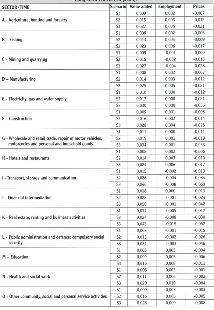
Table 3.1 provides a summary of these results, by focusing on the cumulated long-term (10 years) effects in the three scenarios, expressed in terms of percentage deviations from control. As stated in section 2.1.3, percent deviations from control provide information on the relative size of the expected effects. Since the different sectors have a different weight in the total economy, volumes (value added at constant prices, or jobs) can provide a different picture from that expressed by the measure adopted in the table.

(24)

24

Table 3.1 - Cumulative deviation from control in value added, employment and prices. Long-term effects (10 years).

SECTOR/TIME

A - Agriculture, hunting and forestry B – Fishing

C - Mining and quarrying D – Manufacturing

E - Electricity, gas and water supply F – Construction

G - Wholesale and retail trade, repair of motor vehicles, motorcycles and personal and household goods H - Hotels and restaurants

I - Transport, storage and communication J - Financial intermediation

K - Real estate, renting and business activities

L - Public administration and defence; compulsory social security

M – Education

N - Health and social work

O - Other community, social and personal service activities

Scenario Value added Employment Prices

S1 0,009 0,002 -0,007 S2 0,015 0,003 -0,012 S3 0,027 0,005 -0,021 S1 0,008 0,002 -0,005 S2 0,013 0,004 -0,009 S3 0,023 0,006 -0,017 S1 0,009 -0,001 -0,009 S2 0,015 -0,002 -0,016 S3 0,027 -0,004 -0,028 S1 0,008 0,002 -0,007 S2 0,014 0,003 -0,012 S3 0,025 0,005 -0,021 S1 0,010 0,000 -0,012 S2 0,017 0,000 -0,021 S3 0,030 0,000 -0,035 S1 0,009 0,001 -0,008 S2 0,016 0,002 -0,014 S3 0,028 0,004 -0,025 S1 0,011 0,000 -0,011 S2 0,019 0,001 -0,019 S3 0,034 0,001 -0,033 S1 0,008 0,002 -0,006 S2 0,014 0,003 -0,010 S3 0,024 0,006 -0,017 S1 0,015 -0,002 -0,019 S2 0,026 -0,004 -0,034 S3 0,046 -0,008 -0,060 S1 0,016 0,000 -0,013 S2 0,028 -0,001 -0,024 S3 0,050 -0,001 -0,042 S1 0,014 -0,005 -0,017 S2 0,024 -0,008 -0,030 S3 0,043 -0,015 -0,052 S1 0,008 -0,001 -0,015 S2 0,013 -0,002 -0,026 S3 0,024 -0,003 -0,046 S1 0,005 0,003 -0,004 S2 0,009 0,005 -0,006 S3 0,016 0,008 -0,011 S1 0,006 0,003 -0,001 S2 0,011 0,006 -0,002 S3 0,020 0,010 -0,004 S1 0,009 0,003 -0,003 S2 0,016 0,005 -0,005 S3 0,028 0,009 -0,008

(25)

25

We can summarize the output and employment results in the following points:

1. Output

• The biggest effects in volumes (euro at 2015 prices) are observed for sector D (Manufacturing) and for sector K (Real estate, renting and business activities). The latter result, which has been noted in other studies, is only apparently surprising, since the computer activities belong to this one-digit sector.

• The stronger effects in percentage deviations from control are instead obtained for sector J (Financial intermediation), sector I (Transport, storage and communication) and again sector K (Real estate, renting and business activities). Considering the latter sector, two-digit results show that the strength of the effects for this sector is mainly due to strongly positive effects on the Computer and related activities sector.

2. Employment

• The biggest positive effects in volumes are observed for sector H (Hotel and restaurants) and D (Manufacturing). Employment effects in sector K (Real estate, renting and business activities) are quite strong, smaller than those of the abovementioned sectors. Strongly negative employment effects are observed in sector L (Public administration and defence; compulsory social security). Negative employment effects are observed also in sector I (Transport, storage and communication) and in sector J (Financial intermediation). By construction, the sector-specific employment effects depend on the difference between output (demand) variation and the sector-specific change in productivity. The negative effect in employment are thus observed in those sectors where the increase in BNs increases the output potential more than it increases sector-specific demand.

• The stronger positive effects in percentage deviations from control are instead obtained for sector N (Health and social work), sector M (Education) and sector O (other community, social and personal service activities). Negative deviations from control are stronger in sector K (Real estate, renting and business activities), sector I (Transport, storage and communication) and in sector L (Public administration and defence; compulsory social security).

(26)

26

SECTOR/TIME

M – Education

O - Other community, social and personal service activities Total Scenario Q1 Q4 Q20 Q40 S1 0,002 0,077 0,473 -0,116 S2 0,003 0,135 0,854 -0,210 S3 0,006 0,238 1,509 -0,346 S1 0,000 0,004 0,026 -0,006 S2 0,000 0,007 0,046 -0,011 S3 0,000 0,013 0,082 -0,019 S1 0,002 0,075 0,466 -0,114 S2 0,003 0,133 0,841 -0,207 S3 0,006 0,234 1,487 -0,341 S1 0,034 1,328 8,191 -2,006 S2 0,060 2,337 14,799 -3,646 S3 0,105 4,116 26,151 -6,001 S1 0,003 0,108 0,666 -0,163 S2 0,005 0,190 1,202 -0,296 S3 0,009 0,334 2,124 -0,488 S1 0,005 0,192 1,187 -0,291 S2 0,009 0,339 2,145 -0,528 S3 0,015 0,597 3,790 -0,870 S1 0,003 0,117 0,722 -0,177 S2 0,005 0,206 1,305 -0,322 S3 0,009 0,363 2,306 -0,529 S1 0,002 0,092 0,570 -0,140 S2 0,004 0,163 1,029 -0,254 S3 0,007 0,286 1,819 -0,417 S1 0,007 0,281 1,731 -0,424 S2 0,013 0,494 3,128 -0,771 S3 0,022 0,870 5,527 -1,268 S1 0,006 0,224 1,384 -0,339 S2 0,010 0,395 2,500 -0,616 S3 0,018 0,695 4,418 -1,014 S1 0,036 1,419 8,754 -2,144 S2 0,064 2,497 15,815 -3,896 S3 0,113 4,399 27,948 -6,413 S1 0,002 0,095 0,585 -0,143 S2 0,004 0,167 1,057 -0,260 S3 0,008 0,294 1,867 -0,428 S1 0,001 0,040 0,245 -0,060 S2 0,002 0,070 0,442 -0,109 S3 0,003 0,123 0,781 -0,179 S1 0,002 0,083 0,511 -0,125 S2 0,004 0,146 0,924 -0,228 S3 0,007 0,257 1,632 -0,375 S1 0,002 0,091 0,562 -0,138 S2 0,004 0,160 1,016 -0,250 S3 0,007 0,283 1,796 -0,412 S1 0,108 4,226 26,072 -6,385 S2 0,191 7,438 47,103 -11,605 S3 0,336 13,102 83,238 -19,099

Table 3.2 - Instantaneous output variations: millions euro

(27)

27

Figure 6 - Cumulative output variations: deviations from control

!"!!!# !"!!$# !"!!%# !"!!&# !"!!'# !"!(!# !"!($# !"!(%# !"!(&# )#*#)+,-./01/,2"#3/454+#647# 89,2:1,;# <#=#>-:3-4+# ?#*#@-4-4+#647#A/6,,;-4+# B#=#@64/86.1/,-4+# C#*#C02.1,-.-1;"#+6:#647#D612,# :/EE0;# >#=#?94:1,/.594# F#*#G3902:602#647#,216-0#1,672"# ,2E6-,#98#H919,#I23-.02:"# J#*#J9120:#647#,2:16/,641:## K#*#L,64:E9,1"#:19,6+2#647# .9HH/4-.6594# M#*#>-464.-60#-412,H27-6594# N#*#O260#2:1612"#,2454+#647# P/:-42::#6.5I-52:## Q#*#R/P0-.#67H-4-:1,6594#647# 72824.2S#.9HE/0:9,;#:9.-60# @#=#C7/.6594# T#*#J26013#647#:9.-60#D9,U# V#*#V132,#.9HH/4-1;"#:9.-60# 647#E2,:9460#:2,I-.2#6.5I-52:W# X(# X%# X$!# X%!# !"!!!# !"!!$# !"!%!# !"!%$# !"!&!# !"!&$# !"!'!# (#)#(*+,-./0.+1"#2.343*#536# 78+190+:# ;#<#=,92,3*# >#)#?,3,3*#536#@.5++:,3*# A#<#?53.75-0.+,3*# B#)#B/1-0+,-,0:"#*59#536#C501+# 9.DD/:# =#<#>8390+.-483# E#)#F28/195/1#536#+105,/#0+561"# +1D5,+#87#G808+#H12,-/19"# I#)#I801/9#536#+1905.+5309## J#)#K+539D8+0"#908+5*1#536# -8GG.3,-5483# L#)#=,353-,5/#,301+G16,5483# M#)#N15/#190501"#+1343*#536# O.9,3199#5-4H,419## P#)#Q.O/,-#56G,3,90+5483#536# 61713-1R#-8GD./98+:#98-,5/# ?#<#B6.-5483# S#)#I15/02#536#98-,5/#C8+T# U#)#U021+#-8GG.3,0:"#98-,5/# 536#D1+9835/#91+H,-1#5-4H,419V# W%# WX# W&!# WX!# !"!!!# !"!$!# !"!%!# !"!&!# !"!'!# !"!(!# )#*#)+,-./01/,2"#3/454+#647# 89,2:1,;# <#=#>-:3-4+# ?#*#@-4-4+#647#A/6,,;-4+# B#=#@64/86.1/,-4+# C#*#C02.1,-.-1;"#+6:#647#D612,# :/EE0;# >#=#?94:1,/.594# F#*#G3902:602#647#,216-0# 1,672"#,2E6-,#98#H919,# I#*#I9120:#647#,2:16/,641:## J#*#K,64:E9,1"#:19,6+2#647# .9HH/4-.6594# L#*#>-464.-60#-412,H27-6594# M#*#N260#2:1612"#,2454+#647# O/:-42::#6.5P-52:## Q#*#R/O0-.#67H-4-:1,6594#647# 72824.2S#.9HE/0:9,;#:9.-60# @#=#C7/.6594# T#*#I26013#647#:9.-60#D9,U# V#*#V132,#.9HH/4-1;"#:9.-60# 647#E2,:9460#:2,P-.2# W$# W'# W%!# W'!# Scenario 1 Scenario 2 Scenario 3 ! ! ! ! ! ! KL! KM! KN"! KM"! ! ! ! ! ! ! ! KM! KN"! KM"! ! ! ! ! ! ! ! ! KN"! KM"! ! ! ! ! ! ! ! ! ! KM"! ! ! ! ! ! ! KL! KM! KN"! KM"! ! ! ! ! ! ! ! KM! KN"! KM"! ! ! ! ! ! ! ! ! KN"! KM"! ! ! ! ! ! ! ! ! ! KM"! ! ! ! ! ! ! KL! KM! KN"! KM"! ! ! ! ! ! ! ! KM! KN"! KM"! ! ! ! ! ! ! ! ! KN"! KM"! ! ! ! ! ! ! ! ! ! KM"!

(28)

28

SECTOR/TIME

M – Education

O - Other community, social and personal service activities Total Scenario Q1 Q4 Q20 Q40 S1 0,002 0,130 6,478 7,889 S2 0,003 0,229 11,577 13,787 S3 0,006 0,403 20,427 24,137 S1 0,000 0,007 0,351 0,428 S2 0,000 0,012 0,628 0,748 S3 0,000 0,022 1,108 1,310 S1 0,002 0,128 6,380 7,769 S2 0,003 0,226 11,403 13,579 S3 0,006 0,397 20,121 23,776 S1 0,034 2,255 112,239 136,683 S2 0,060 3,969 200,595 238,871 S3 0,105 6,991 353,918 418,196 S1 0,003 0,183 9,120 11,106 S2 0,005 0,323 16,298 19,408 S3 0,009 0,568 28,752 33,973 S1 0,005 0,327 16,267 19,809 S2 0,009 0,575 29,071 34,618 S3 0,015 1,013 51,289 60,604 S1 0,003 0,199 9,898 12,053 S2 0,005 0,350 17,690 21,065 S3 0,009 0,617 31,211 36,879 S1 0,002 0,157 7,808 9,509 S2 0,004 0,276 13,955 16,617 S3 0,007 0,486 24,619 29,090 S1 0,007 0,477 23,722 28,888 S2 0,013 0,839 42,396 50,486 S3 0,022 1,478 74,802 88,387 S1 0,006 0,381 18,959 23,088 S2 0,010 0,670 33,884 40,349 S3 0,018 1,181 59,784 70,643 S1 0,036 2,410 119,949 146,073 S2 0,064 4,242 214,377 255,283 S3 0,113 7,472 378,240 446,937 S1 0,002 0,161 8,014 9,760 S2 0,004 0,283 14,323 17,056 S3 0,008 0,499 25,270 29,860 S1 0,001 0,067 3,352 4,082 S2 0,002 0,119 5,991 7,135 S3 0,003 0,209 10,571 12,491 S1 0,002 0,141 7,005 8,531 S2 0,004 0,248 12,520 14,909 S3 0,007 0,436 22,090 26,101 S1 0,002 0,155 7,707 9,386 S2 0,004 0,273 13,775 16,403 S3 0,007 0,480 24,304 28,718 S1 0,108 7,178 357,248 435,055 S2 1,191 16,634 658,487 760,313 S3 0,336 22,253 1126,507 1331,103

(29)

ASSESSING THESECTORALEFFECTS OFICTINVESTMENTS- THECASE OFBROADBANDNETWORKS

29

3.3 - Selected results: employment variations

SECTOR/TIME

G - Wholesale and retail trade, repair of motor vehicles, motorcycles and personal an